Theory of charged impurity scattering in two dimensional graphene
Abstract
We review the physics of charged impurities in the vicinity of graphene. The long-range nature of Coulomb impurities affects both the nature of the ground state density profile as well as graphene’s transport properties. We discuss the screening of a single Coulomb impurity and the ensemble averaged density profile of graphene in the presence of many randomly distributed impurities. Finally, we discuss graphene’s transport properties due to scattering off charged impurities both at low and high carrier density.
I Introduction
Graphene is a two dimensional sheet of carbon whose atoms arrange in a honeycomb lattice with nearest neighbor atoms forming strong sp2 bonds. The electronic properties of this material are mostly determined by the orbitals with each carbon atom contributing one electron to a Bloch band whose low energy properties are adequately described by a Dirac-Weyl effective Hamiltonian. While the study of Dirac Fermions has emerged in several contexts in theoretical condensed matter physics, its experimental realization about three years ago, in the form of gated graphene devices, [1, 2, 3] where the carrier density can be tuned continuously from electron-like carriers for positive bias to hole-like carriers for negative gate voltage, has prompted a prolific theoretical and experimental effort to understand the properties of this novel material.
Most of excitement surrounding graphene stems from one of the following peculiar properties: (i) Electrons and holes in graphene have a gapless linear dispersion relation in contrast to the parabolic dispersion of other more conventional electron gases; (ii) The carriers in graphene are chiral – a property that has striking consequences such as the “half-integer” quantum Hall Effect [2, 3]; and (iii) Carriers in graphene live at an exposed almost perfect D surface that is amenable to surface probes [4, 5, 6, 7, 8] and surface manipulation. [9, 10] In addition, we note that there is the potential of mass producing graphene through epitaxial growth methods, [11] and that graphene has remarkable mechanical properties [12, 13] which only further enhance the interest.
In this Perspective, we look at one important aspect of graphene which is the influence of disorder on its ground state and transport properties. We demonstrate that for graphene, charged (i.e. Coulomb) impurities behave qualitatively different from neutral impurities [14, 15, 16] and dominate graphene’s transport properties at low carrier density. The importance of the Coulomb nature of graphene impurities was first highlighted by Ando, [17] where by calculating the intraband contribution to the polarizability and absorbing the interband (i.e. electron-hole) contribution into a redefinition of the dielectric constant [18] he showed that charged impurities could explain the conductivity being linear-in-density as was seen in experiments. [1, 19] Similar conclusions were obtained by Nomura and MacDonald [20] using a “complete screening” model (i.e. ), Cheianov and Falko using a numerical Thomas-Fermi approximation [21] and in Ref. 22 using the full Random-Phase-Approximation (RPA). Analytic expressions for the RPA polarizability function calculated first in Ref. 23 and then in Refs. 24, 25, 26 revealed that for momentum transferred on the Fermi circle (i.e. ) the graphene dielectric function calculated using the RPA was identical to the much simpler Thomas-Fermi approximation at (see Fig. 1). This then made it possible to calculate the RPA-Boltzmann conductivity analytically, [27] and the dependence of graphene’s conductivity on the fine-structure constant was recently verified experimentally. [10] The importance of Coulomb scattering in explaining the observed graphene transport properties soon prompted an interest in investigating the properties of a single charged impurity embedded in graphene. Katsnelson [28] studied this problem using a Fermi-Thomas approximation, followed by studies in Refs. 29, 30, 31, 32, 33, 34, 35 who were mostly interested in effects beyond the RPA such as determining the critical impurity charge for which the Coulomb impurity forms bound states and the screening properties of graphene in the supercritical regime.

It was understood by Refs. 22, 36 that as one approached the Dirac point, one would soon encounter a situation where the gate voltage induced carrier density would be smaller than the fluctuation of carrier density induced by the charged impurities thereby breaking the graphene landscape into puddles of electrons and holes. Solving numerically for the conductivity using a finite-sized Kubo formalism for a limited range of impurity concentrations, Ref. 36 concluded that the Coulomb disorder model gave a universal minimum conductivity whose value did not depend on the charged impurity concentration, but that was larger than that expected for clean Dirac Fermions, [37, 38, 39, 28, 40] while Ref. 22 argued that this would give rise to a non-universal minimum conductivity whose value depended on the concentration of charged impurities. Ref. 27 developed a mean field approach to understand the properties of graphene at the Dirac point by calculating an effective carrier density self-consistently. This theory made quantitative predictions about the dependence of the minimum conductivity and rms carrier density on the charged impurity concentration and substrate dielectric constant, and in particular argued that cleaner graphene samples would have larger minimum conductivity. Ref. 41 then studied the ground state properties of graphene by minimizing an energy functional comprising kinetic energy, Hartree, exchange [42, 25, 43] and correlation [25, 43, 44] contributions in the presence of Coulomb disorder. This work made quantitative predictions about properties of the carrier density distribution, both at and away from the Dirac point, and enabled Ref. 45 to develop an effective medium theory to calculate the graphene’s conductivity through these inhomogeneous puddles, capturing quantitatively the minimum conductivity plateau that is seen in experiments. [1, 19, 46] We mention that underlying the existence of this minimum conductivity plateau is the high transmission of graphene p-n junctions, which has been the subject of theoretical [47, 48] and experimental study. [49, 50, 51] For the purposes of this paper we do not discuss quantum interference effects (see Ref. 52 and references therein) or the strongly interacting regime (see Ref. 53 and references therein).
The remainder of this paper is structured as follows. In Section II we discuss the problem of the screening of a single Coulomb impurity in the sub-critical regime as a useful toy model to understand the many impurity problem that we address in Section III where we study the case of many Coulomb impurities that are uncorrelated and distributed uniformly in order to study the ground state properties of graphene. In Section IV.1, we review the high-density Boltzmann transport theory, and discuss the Effective Medium Theory (EMT) in Section IV.2. In Sections V, VI, and VII we briefly review the experimental situation, discuss graphene minimum conductivity, and recent theoretical work not covered in this review. We then conclude in Section VIII.
II Screening of a single Coulomb impurity
Following Ref. 28 one can construct the Thomas-Fermi screening of a single charged impurity. The goal is to calculate the screened Coulomb potential , where the bare potential and the induced potential is given by
| (1) |
where we can imagine tuning the back gate to ensure charge neutrality . If one further assumes that the local carrier density is given by the Fermi-Thomas condition, , one can write down a (one dimensional) self-consistency equation for
| (2) |
where is the complete elliptic integral of the first kind. The screened potential induced for this single impurity using this method was discussed in Ref. 28. This formalism can be generalized using the method developed in Ref. 41 to include the effects of exchange. The ground state carrier density can be obtained from the Thomas-Fermi-Dirac (TFD) energy functional
| (3) | |||||
where the first term in Eq. 3 is the kinetic energy, the second term is the Hartree part of the Coulomb interaction, the third is the exchange-correlation energy and the fourth term is the energy due to disorder, where is the disorder potential and the last term is added to set the average carrier density, , through the chemical potential . The correlation term is much smaller than exchange and, to very good approximation [25, 43, 44] is proportional to exchange. Therefore, hereafter, we neglect the correlation contribution by assuming , where is the Hartree-Fock self-energy. [25, 43, 42] The energy functional Eq. 3 is quite general and can be tailored by properly choosing and its coupling to , to consider different sources of disorder. For the single impurity problem, the solution can also be cast as a one dimensional integral equation
| (4) | |||||
where is the band energy cutoff and .
III Ground state properties at the Dirac point
The single impurity problem discussed in the previous section is a much simpler problem because rotational symmetry makes the problem one-dimensional. Adding many impurities also brings further complications: while the carrier density induced by a single impurity is negligible, this is not the case for many impurities where although the average density can be tuned to zero via an external gate potential, the scale of the density fluctuations is set by the impurity concentration. [22] As shown in Fig. 1, the RPA screening properties of graphene are very different at the Dirac point (i.e. ) and at finite density, therefore theoretical frameworks constructed to work at the Dirac point are bound to fail when there are such large density fluctuations. In this section, we present two different approaches to describe the Dirac point. The first is a mean-field theory where an effective density is obtained by solving self-consistently for the density induced by the fluctuations of the screened impurity potential (that itself depends on density). The second is a generalization of the energy functional method discussed above for a single impurity to the much more complicated case of many Coulomb impurities.
III.1 Self-consistent Approximation (SCA)
For any microscopic single impurity potential , the probability distribution, , of the total potential, , is where is the average over all possible disorder configurations. Assuming that the impurities positions are uncorrelated one can compute expressions for all moments of the induced disorder potential. [54, 55] For example, the connected moment . The self-consistent approximation involves obtaining the effective carrier density by equating the second moment of the disorder potential with the square of the corresponding Fermi energy . This self-consistent approximation then allows us to compute any correlation function at the Dirac point, although closed form analytic results are often elusive. To make analytical progress, one can map
| (5a) | |||||
| (5b) | |||||
where analytic expressions for and , were reported in Ref. 56. A numerical evaluation of Eq. 5a and the Gaussian approximation Eq. 5b is shown in Fig. 2. Within the Gaussian approximation one finds that , where in the last equation we further assume that . This result for is particularly useful when comparing the self-consistent approximation with other methods.

III.2 Energy Functional Minimization (EFM)
To study graphene transport properties for a distribution of charged impurities, we use Eq. 3 taking to be the potential generated by a random 2D distribution of impurity charges placed at a distance from the graphene layer. We assume to be on average zero and uncorrelated and perform our calculations on a 200 nm200 nm square sample with a 1 nm spatial discretization. Close to the Dirac point, for a single disorder realization, we find that the carrier density breaks up into electron-hole puddles. Since we are interested in disorder averaged quantities, we examine several disorder realizations (500-1000) and denote disordered averaged quantities by angled brackets. To characterize the density profile, we calculate the disorder averaged density-density correlation function , from which we can extract the root mean square , and the typical correlation length, , defined in this section as the FWHM of . We find [41] for typical graphene samples, that for dopings as high as cm-2 and that close to the Dirac point, for cm-2, including exchange is three times smaller than without. We find the correlation length to be of the order of nm, see Fig. 3. This value suggest that the electron-hole puddles are quite small. However a closer inspection reveals that, close to the Dirac point, the density profile is characterized by two distinct types of inhomogeneities [45]: wide regions (i.e. big puddles spanning the system size) of low density containing a number of electrons (holes) of order 10; and few narrow regions, whose size is correctly estimated by , of high density containing a number of carriers of order 2. This picture is confirmed by the results shown in Fig. 4 in which the disorder averaged area fraction, , over which is plotted as a function of . We see that is of order 1/3 and we also find that the area fraction over which is less than of is close to 50% for cm-2. The combination of the relatively high density in the peaks/dips and the fact that in the low density regions varies over scales much bigger than guarantees that the inequality is satisfied over the majority of the graphene sample and therefore justifies the use of the EFM theory. The EFM should be a reasonable quantitative theory for existing graphene samples at all values of the carrier density.


III.3 Comparison of SCA and EFM
Here we compare the results from the Self-Consistent Approximation of Sec. III.1 and the Energy Functional Minimization (EFM) formalism discussed in Sec III.2. Figure 2 shows the disordered averaged spatial correlation function at the Dirac point for the screened disorder potential where the (red) diamonds are obtained minimizing Eq. 3. The solid (blue) line shows the same quantity calculated using the self-consistent approximation (SCA). The EFM approach and the SCA give a similar behavior for , characterized by an algebraic, , decay at large distances. The green solid line shows a Gaussian approximation which captures much of the quantitative details of the screened disorder potential correlation function, but not the power law decay.


In Figs. 5 -7, at the Dirac point is shown as function of , and respectively. The red dashed lines show the results obtained using the EFM theory including exchange, the solid blue lines are the results obtained using the SCA theory. In general the SCA gives values of smaller than the EFM theory but in general there is good semi-quantitative agreement especially at low and .
IV Graphene Conductivity
IV.1 High-density: Boltzmann Transport Theory
In this section we investigate the graphene transport for large carrier densities (), where the system is homogeneous. We show in detail the microscopic transport properties at high carrier density using the Boltzmann transport theory. [57] We calculate the conductivity (or mobility ) in the presence of randomly distributed Coulomb impurity charges near the surface with the electron-impurity interaction being screened by the 2D electron gas in the random phase approximation (RPA). Even though the screened Coulomb scattering is the most important scattering mechanism in our calculation, there are additional scattering mechanisms (i.e. neutral point defects) unrelated to the charged impurity scattering for very high mobility samples. Point defects gives rise to a constant conductivity in contrast to charged impurity scattering which produces a conductivity linear in . Our formalism can include both effects, where zero range scatterers are treated with an effective point defect density of . For the purpose of this calculation, we neglect all phonon scattering effects, which were considered recently with the finding that acoustic phonon scattering gives rise to a resistivity that is linear in temperature. [58]
We start by assuming graphene to be a homogeneous 2D carrier system of electrons (or holes) with a carrier density induced by the external gate voltage. The low-energy band Hamiltonian for homogeneous graphene is well-approximated by a 2D Dirac equation for massless particles,
| (6) |
where is the 2D Fermi velocity, and are Pauli spinors and is the momentum relative to the Dirac points. The corresponding eigenstates are given by the plane wave , where is the area of the system, indicate the conduction () and valence () bands, respectively, and with being the polar angle of the momentum . The corresponding energy of graphene for 2D wave vector is given by , and the density of states (DOS) is given by , where is the total degeneracy ( being the spin and valley degeneracies, respectively).
When the external force is weak and the displacement of the distribution function from the thermal equilibrium value is small, we can use linearized Boltzmann equation within relaxation time approximation. In this case the conductivity for graphene can be written by
| (7) |
Note that is the Fermi distribution function, where the finite temperature chemical potential is determined self-consistently to conserve the total number of electrons. At , is a step function at the Fermi energy , and we then recover the Einstein relation . In Eq. (7) is the relaxation time or the transport scattering time of the collision and is given by
| (8) | |||||
where is the scattering angle between the scattering in- and out- wave vectors and , and is the matrix element of the scattering potential associated with impurity disorder in the graphene environment, and is the number of impurities per unit area of the -th kind of impurity. Note that since we consider the elastic impurity scattering the interband processes () are not permitted.
The matrix element of the scattering potential of randomly distributed screened impurity charge centers in graphene is given by
| (9) |
where , , and is the Fourier transform of the 2D Coulomb potential in an effective background lattice dielectric constant , where is the location of the charged impurity measured from the graphene sheet. The factor arises from the sublattice symmetry (overlap of wave function). [17]
In Eq. (9), is the 2D finite temperature static RPA dielectric (screening) function appropriate for graphene, given by , where is the graphene irreducible finite-temperature polarizability function, [58] is the Coulomb interaction, and is the local field correction. In RPA, and in Hubbard approximation (HA), . [59]

In Fig. 8 we show the calculated graphene conductivities limited by screened charged impurities. The RPA screening used in our calculation is the main approximation. We also show results for HA screening [59] which includes local field corrections approximately. We note that since the graphene is a weakly interacting system () the correlation effects are not strong. We emphasize that in order to get quantitative agreement with experiment, the screening effects must be included. Using the unscreened dielectric function would have conductivity less than for the entire range of gate voltages used in the experiment. Our main result with screened Coulomb impurities is the quantitative agreement with experiments in the regime where the conductivity is linear in density. In inset we show the effect of remote scatterers which are located at a distance from the interface. The main effect of remote impurity scatterings is that the conductivity deviates from the linear behavior with density and increases with both the distance and .


For very high mobility samples, one finds a sub-linear conductivity instead of the linear behavior with density. Such high quality samples presumably have a small charge impurity concentration and it is therefore likely that point defects here play a more dominant role. Point defects gives rise to a constant conductivity in contrast to charged impurity scattering which produces a conductivity linear in . In the presence of both the long-ranged charged impurity and the short-ranged neutral impurity, the total scattering time becomes where () is the scattering time due to charged Coulomb (short ranged) impurities. Shown in Fig. 9 is the graphene conductivity calculated including both charge impurity and zero range point defect scattering for different ratios of the point scatterer impurity density and the charge impurity density . For small we find the linear conductivity that is seen in most experiments and for large we see the flattening out of the conductivity curve (which in the literature [3] has been referred to as the sub-linear conductivity). We believe this high-density flattening of the graphene conductivity is a non-universal crossover behavior arising from the competition between two kinds of scatterers. In general this crossover occurs when two scattering potentials are equivalent, that is, .
In the inset of Fig. 9 we show our calculated mobility in the presence of both charged impurities and short-ranged impurities. As the scattering limited by the short-ranged impurity dominates over that by the long-ranged impurity (e.g. ) the mobility is no longer dependent on the charged impurity and approaches its limiting value
| (10) |
The limiting mobility depends only on neutral impurity concentration and carrier density, which indicates that to get high graphene mobility it is necessary to have defect free graphene.
Finally in Fig. 10 we show the calculated temperature dependent conductivity for different temperatures as a function of density. We note that there are two independent sources of temperature dependent resistivity in our calculation. One comes from the energy averaging defined in Eq. (7), and the other is the explicit temperature dependence of the dielectric function which produces a temperature dependent . Figure 10 shows that in the high density limit the conductivity decreases as the temperature increases, but in the low density limit the conductivity shows non-monotonic behavior, i.e. has a local minimum at a finite temperature and increases as the temperature increases. Thus, we find that the calculated conductivity shows a non-monotonicity in the low density limit, i.e., at low temperatures the conductivity shows metallic behavior and at high temperatures it shows insulating behavior. The non-monotonicity of temperature dependent is understood to arise from temperature dependent screening. [60] We mention that for K, phonons contribute to the temperature dependence of graphene conductivity. [58, 61]
IV.2 Low Density: Effective Medium Theory
At low density the fluctuations in carrier density become larger than the average density. To understand the transport properties of this inhomogeneous system, Ref. 45 developed an effective medium theory where graphene’s conductivity is found by solving an integral equation
| (11) |
where is the density distribution function and is the (local) Boltzmann conductivity discussed in Sec. IV.1. For the purpose of this section, we take where was derived in Ref. 27 and shown in Fig. 11. The quantitatively accurate theory using derived from the EFM of Sec III.2 was developed in Ref. 45. Here we derive analytical results obtained by using model distribution functions for , which as discussed in Ref. 45 show quantitative agreement with the numerical theory only for small and low . To illustrate this method, we first consider to be a Gaussian distribution. Requiring that fixes all the free parameters. Solving Eq. 11 then gives , where is the imaginary error function, is the exponential integral function and giving , where we use the results of Sec. III.1 that and . The development of an effective medium theory for graphene [45] now allows us to reinterpret the results of Ref. 27 as equivalent to the assumption that is Gaussian with density fluctuations determined by the self-consistency condition .

We can explore other functional forms for . For a Lorentzian , one can solve Eq. 11 analytically giving . If one identifies the width of the Lorentzian with the self-consistent carrier density , then this provides another way to understand the self-consistent transport result. Subsequent to the results of Ref. 45, Fogler developed an effective medium theory using , where similar to the Gaussian distribution case, requiring normalization and setting fixes all the free parameters. Solving Eq. 11 gives where is the Gamma function and . Again, approximating , we find , which is different from the numerical results obtained in Ref. 62. While these analytical approximations are useful in providing a qualitative understanding of graphene transport, quantitative differences remain between these and the full numerical solution [45] especially at large impurity concentrations and large (See e.g. Fig. 6).
IV.3 Suspended Graphene
One of the direct consequences of charged impurity scattering in graphene is the prediction [22] that the elimination of charged impurities from the graphene environment, for example, by suspending graphene, without any substrate would lead to a much enhanced carrier mobility. Recently, Bolotin et al. [63, 64] managed to remove charged impurities from the graphene environment by suspending graphene without any substrate (and simply current-annealing away any remnant impurities on the graphene surface). This immediately led to an oder of magnitude increase (to ) in the graphene mobility as predicted theoretically. Recent theoretical work [65] shows excellent agreement with the transport measurements on suspended graphene, [63, 64, 66] with both the reduced impurity density and the modified screening (due to the elimination of the substrate) contributing to the graphene conductivity. Since phonon scattering effects in graphene are weak upto room temperature, [58] the enhanced graphene mobility arising from the elimination of charged impurities may lead to very high () graphene mobilities even at room temperature.
V Discussion of experiments
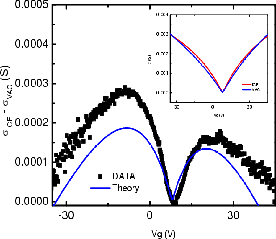
One of the very first puzzles in graphene transport experiments [1] was that the conductivity was linear in carrier density, whereas existing theory [39] predicted constant conductivity at high density. As discussed in the introduction, the linear in density emerges naturally from the Boltzmann transport theory of charged impurities, [17, 20, 21, 22, 27] and to our knowledge, no other theory produces this linear behavior without a fine-tuning of parameters to make the scattering mimic Coulomb impurities. Moreover, three recent experiments have rigorously verified the high density predictions of the Boltzmann transport theory. In Ref. 19 sample mobility was correlated with shift of the Dirac point and plateau width showing qualitative and semi-quantitative agreement with the theory presented here. Reference 46 were able to directly measure the effect of Coulomb scatterers by intentionally adding potassium ions to graphene in ultra-high vacuum observing qualitatively all the predictions of the (self-consistent) Boltzmann theory. Finally, Ref. 10 was able to tune graphene’s fine structure constant by depositing ice on top of graphene, and thereby precisely testing predictions of the Boltzmann theory. Results from this experiment are shown in Fig 12. Since the dielectric constant of the SiO2 substrate and that of ice are known, there are no adjustable parameters in the theoretical curve.
VI The Minimum Conductivity Puzzle
As described above in Sec. IV.2, our recent theoretical work [27, 45] provides a satisfactory explanation for the minimum conductivity phenomenon in graphene near the charge neutrality (i.e. Dirac) point. In particular, early theoretical work [37, 38, 39, 28, 40] predicted a universal minimum conductivity at the graphene Dirac point in clean disorder-free systems. The inclusion of disorder-induced quantum anti-localization effect, assuming no intervalley scattering, leads to a theoretical infinite minimum conductivity at the Dirac point, whereas the presence of inter-valley scattering localizes the system leading to zero conductivity at the Dirac point. This confusing theoretical picture stands in stark contrast to the experimental reality, where the graphene conductivity is approximately a constant (as a function of gate voltage or carrier density) around the Dirac point, with this constant minimum conductivity plateau having a non-universal sample dependent value ().
It was first suggested in Ref. 22 that the minimum conductivity phenomenon is closely related to the break-up of the graphene landscape into inhomogeneous puddles of electrons and holes around the Dirac point due to the effect of the charged impurities in the environment. This physical idea was further developed into a quantitatively successful theory (see Sec. IV.2 above) in Refs. 27, 45, where it was shown that a self-consistent treatment of the impurity induced electron-hole puddles coupled with the Boltzmann transport theory provides excellent description of the non-universal behavior of the minimum conductivity around the Dirac point. In particular, the sample dependence of the minimum conductivity arises from the different impurity disorder in different samples.
Quantum effective field theories of graphene minimum conductivity, which predict a universal minimum conductivity, are inapplicable to real graphene samples because real graphene is dominated by disorder induced inhomogeneity near the Dirac point, which is outside the scope of the quantum field theories. Although the self-consistent effective medium theory developed by us [27, 45] gives reasonable agreement with the experimental observations, the key conceptual question of what happens at as disorder also goes to zero still remains open. Such a scenario is of course experimentally irrelevant (since experiments are performed at finite temperatures in disordered systems), but the theoretical question of the conductivity crossover from the inhomogeneous Boltzmann regime of Refs. 27, 45 to the homogeneous quantum transport regime is an interesting open question. Recent attempts to understand such crossover phenomena include several complementary theoretical avenues (See Refs. 52, 67, 53 and references therein).
VII Recent Work
Among recent relevant work not discussed in this review we mention a detailed calculation of the temperature dependent graphene conductivity due to electron-phonon scattering, [58] a detailed calculation of the temperature dependent graphene conductivity due to the temperature dependence of the screening of charged impurity scattering, [60] a calculation of graphene density of states as modified by impurity scattering, [68] a consideration of percolation induced localization transition in graphene nanoribbons, [56] a theory of charged impurity screening in graphene bilayers, [69] and a prediction of graphene magnetoresistance induced by a parallel magnetic field through the spin-polarization dependence of screening. [70]
VIII Conclusion
We have developed here the theory for Coulomb impurities on graphene. As we have shown, Coulomb impurities behave qualitatively different from short-range scatterers such as point defects or missing atoms. Away from the Dirac point, the physics is well described by a semi-classical Boltzmann transport theory, while at the Dirac point density fluctuations dominate breaking the system into puddles of electrons and holes. We have shown how these inhomogeneities can be characterized by a mean-field self-consistent theory and by numerically minimizing graphene’s energy functional, and that an effective medium theory can be employed to describe the low density transport properties giving semi-quantitative agreement with experimental results.
We thank Michael Fuhrer for valuable discussions. This work is supported by US-ONR and NSF-NRI-SWAN.
References
- [1] K. S. Novoselov, A. K. Geim, S. V. Morozov, D. Jiang, Y. Zhang, S. V. Dubonos, I. V. Grigorieva, and A. A. Firsov, Science 306, 666 (2004).
- [2] K. S. Novoselov, A. K. Geim, S. V. Morozov, D. Jiang, Y. Zhang, M. I. Katsnelson, I. V. Grigorieva, S. V. Dubonos, and A. A. Firsov, Nature 438, 197 (2005).
- [3] Y. Zhang, Y.-W. Tan, H. L. Stormer, and P. Kim, Nature 438, 201 (2005).
- [4] M. Ishigami, J. H. Chen, W. G. Cullen, M. S. Fuhrer, and E. D. Williams, Nano Lett. 7, 1643 (2007).
- [5] E. Stolyarova, K. T. Rim, S. Ryu, J. Maultzsch, P. Kim, L. E. Brus, T. F. Heinz, M. S. Hybertsen, and G. W. Flynn, Proc. Nat. Acad. Sci. 104, 9209 (2007).
- [6] G. M. Rutter, J. N. Crain, N. P. Guisinger, T. Li, P. N. First, and J. A. Stroscio, Science 317, 219 (2007).
- [7] G. Li and E. Y. Andrei, Nature Physics 3, 623 (2007).
- [8] J. Martin, N. Akerman, G. Ulbricht, T. Lohmann, J. H. Smet, K. von Klitzing, and A. Yacobi, Nature Physics 4, 144 (2008).
- [9] F. Schedin, A. K. Geim, S. V. Morozov, D. Jiang, E. H. Hill, P. Blake, and K. S. Novoselov, Nature Materials 6, 652 (2007).
- [10] C. Jang, S. Adam, J.-H. Chen, E. D. Williams, S. Das Sarma, and M. S. Fuhrer, Phys. Rev. Lett. 101, 146805 (2008).
- [11] C. Berger, Z. Song, X. Li, X. Wu, N. Brown, C. Naud, D. Mayou, T. Li, J. Hass, A. N. Marchenkov, et al., Science 312, 1191 (2006).
- [12] J. S. Bunch, A. M. van der Zande, S. S. Verbridge, I. W. Frank, D. M. Tanenbaum, J. M. Parpia, H. G. Craighead, and P. L. McEuen, Science 315, 490 (2007).
- [13] C. Lee, X. Wei, J. W. Kysar, and J. Hone, Science 321, 385 (2008).
- [14] I. Aleiner and K. Efetov, Phys. Rev. Lett. 97, 236801 (2006).
- [15] A. Altland, Phys. Rev. Lett. 97, 236802 (2006).
- [16] M. S. Foster and I. L. Aleiner, Phys. Rev. B 77, 195413 (2008).
- [17] T. Ando, J. Phys. Soc. Jpn. 75, 074716 (2006).
- [18] J. Gonzalez, F. Guinea, and V. A. M. Vozmediano, Nucl. Phys. B 424, 595 (1994).
- [19] Y.-W. Tan, Y. Zhang, K. Bolotin, Y. Zhao, S. Adam, E. H. Hwang, S. Das Sarma, H. L. Stormer, and P. Kim, Phys. Rev. Lett. 99, 246803 (2007).
- [20] K. Nomura and A. H. MacDonald, Phys. Rev. Lett. 96, 256602 (2006).
- [21] V. Cheianov and V. Fal’ko, Phys. Rev. Lett. 97, 226801 (2006a).
- [22] E. H. Hwang, S. Adam, and S. Das Sarma, Phys. Rev. Lett. 98, 186806 (2007a).
- [23] E. H. Hwang and S. Das Sarma, Phys. Rev. B 75, 205418 (2007).
- [24] B. Wunsch, T. Stauber, F. Sols, and F. Guinea, New J. Phys. 8, 318 (2006).
- [25] Y. Barlas, T. Pereg-Barnea, M. Polini, R. Asgari, and A. H. MacDonald, Phys. Rev. Lett. 98, 236601 (2007).
- [26] M. Polini, R. Asgari, Y. Barlas, T. Pereg-Barnea, and A. MacDonald, Solid State Commun. 143, 58 (2007).
- [27] S. Adam, E. H. Hwang, V. M. Galitski, and S. Das Sarma, Proc. Natl. Acad. Sci. USA 104, 18392 (2007).
- [28] M. I. Katsnelson, Eur. Phys. J. B 51, 157 (2006).
- [29] A. V. Shytov, M. I. Katsnelson, and L. S. Levitov, Phys. Rev. Lett. 99, 236801 (2007).
- [30] V. M. Pereira, J. Nilsson, and A. H. Castro Neto, Phys. Rev. Lett. 99, 166802 (2007).
- [31] R. R. Biswas, S. Sachdev, and D. T. Son, Phys. Rev. B 76, 205122 (2007).
- [32] D. S. Novikov, Appl. Phys. Lett. 91, 102102 (2007).
- [33] M. M. Fogler, D. S. Novikov, and B. I. Shklovskii, Phys. Rev. B 76, 233402 (2007).
- [34] I. S. Terekhov, A. I. Milstein, V. N. Kotov, and O. P. Sushkov, Phys. Rev. Lett. 100, 076803 (2008).
- [35] V. M. Pereira, V. N. Kotov, and A. H. Castro Neto, Phys. Rev. B 78, 085101 (2008).
- [36] K. Nomura and A. H. MacDonald, Phys. Rev. Lett. 98, 076602 (2007).
- [37] E. Fradkin, Phys. Rev. B 33, 3257 (1986).
- [38] A. W. W. Ludwig, M. P. A. Fisher, R. Shankar, and G. Grinstein, Phys. Rev. B 50, 7526 (1994).
- [39] N. Shon and T. Ando, J. Phys. Soc. Jpn. 67, 2421 (1998).
- [40] J. Tworzydło, B. Trauzettel, M. Titov, A. Rycerz, and C. W. J. Beenakker, Phys. Rev. Lett. 96, 246802 (2006).
- [41] E. Rossi and S. Das Sarma, Phys. Rev. Lett. 101, 166803 (2008).
- [42] E. H. Hwang, B. Y.-K. Hu, and S. Das Sarma, Phys. Rev. Lett. 99, 226801 (2007b).
- [43] S. Das Sarma, E. H. Hwang, and W.-K. Tse, Phys. Rev. B 75, 121406 (2007).
- [44] M. Polini, A. Tomadin, R. Asgari, and A. H. MacDonald, Phys. Rev. B 78, 115426 (2008).
- [45] E. Rossi, S. Adam, and S. Das Sarma, arXiv:0809.1425 (2008).
- [46] J. H. Chen, C. Jang, S. Adam, M. S. Fuhrer, E. D. Williams, and M. Ishigami, Nature Physics 4, 377 (2008a).
- [47] V. Cheianov and V. I. Fal’ko, Phys. Rev. B 74, 041403 (2006b).
- [48] M. M. Fogler, D. S. Novikov, L. I. Glazman, and B. I. Shklovskii, Phys. Rev. B 77, 075420 (2008).
- [49] B. Huard, J. A. Sulpizio, N. Stander, K. Todd, B. Yang, and D. Goldhaber-Gordon, Phys. Rev. Lett. 98, 236803 (2007).
- [50] J. R. Williams, L. DiCarlo, and C. M. Marcus, Science 317, 638 (2007).
- [51] B. Özyilmaz, P. Jarillo-Herrero, D. Efetov, D. A. Abanin, L. S. Levitov, and P. Kim, Phys. Rev. Lett. 99, 166804 (2007).
- [52] S. Adam, P. W. Brouwer, and S. Das Sarma, arXiv:0811.0609v1 (2008a).
- [53] M. Mueller, L. Fritz, and S. Sachdev, arXiv:0805.1413v1 (2008).
- [54] V. Galitski, S. Adam, and S. Das Sarma, Phys. Rev. B 76, 245405 (2007).
- [55] S. Adam and S. Das Sarma, Phys. Rev. B 77, 115436 (2008).
- [56] S. Adam, S. Cho, M. S. Fuhrer, and S. Das Sarma, Phys. Rev. Lett. 101, 046404 (2008b).
- [57] S. Das Sarma and E. H. Hwang, Phys. Rev. Lett. 83, 164 (1999).
- [58] E. H. Hwang and S. Das Sarma, Phys. Rev. B 77, 115449 (2008a).
- [59] M. Jonson, J. Phys. C 9, 3059 (1976).
- [60] E. H. Hwang and S. Das Sarma, arXiv:0811.1212v1 (2008b).
- [61] J. H. Chen, C. Jang, S. Xiao, M. Ishigami, and M. S. Fuhrer, Nature Nanotechnology 3, 206 (2008b).
- [62] M. M. Fogler, arXiv:0810.1755v1 (2008).
- [63] K. Bolotin, K. Sikes, Z. Jiang, G. Fudenberg, J. Hone, P. Kim, and H. Stormer, Solid State Commun. 146, 351 (2008a).
- [64] K. I. Bolotin, K. J. Sikes, J. Hone, H. L. Stormer, and P. Kim, Phys. Rev. Lett. 101, 096802 (2008b).
- [65] S. Adam and S. Das Sarma, Solid State Commun. 146, 356 (2008).
- [66] X. Du, I. Skachko, A. Barker, and E. Andrei, Nature Nanotechnology 3, 491 (2008).
- [67] V. Cheianov, V. Fal’ko, B. Altshuler, and I. Aleiner, Phys. Rev. Lett. 99, 176801 (2007).
- [68] B. Y. Hu, E. H. Hwang, and S. Das Sarma, Phys. Rev. B 78, 165411 (2008).
- [69] E. H. Hwang and S. Das Sarma, Phys. Rev. Lett. 101, 156802 (2008c).
- [70] E. H. Hwang and S. Das Sarma, arXiv:0812.0403v1 (2008d).