The Impact of QoS Constraints on the Energy Efficiency of Fixed-Rate Wireless TransmissionsThanks: The authors are with the Department of Electrical Engineering, University of Nebraska-Lincoln, Lincoln, NE, 68588 (e-mails: qdl726@bigred.unl.edu, gursoy@engr.unl.edu, velipasa@engr.unl.edu).Thanks: This work was supported by the National Science Foundation under Grants CCF – 0546384 (CAREER) and CNS – 0834753.
Abstract
Transmission over wireless fading channels under quality of service (QoS) constraints is studied when only the receiver has channel side information. Being unaware of the channel conditions, transmitter is assumed to send the information at a fixed rate. Under these assumptions, a two-state (ON-OFF) transmission model is adopted, where information is transmitted reliably at a fixed rate in the ON state while no reliable transmission occurs in the OFF state. QoS limitations are imposed as constraints on buffer violation probabilities, and effective capacity formulation is used to identify the maximum throughput that a wireless channel can sustain while satisfying statistical QoS constraints. Energy efficiency is investigated by obtaining the bit energy required at zero spectral efficiency and the wideband slope in both wideband and low-power regimes assuming that the receiver has perfect channel side information (CSI). In the wideband regime, it is shown that the bit energy required at zero spectral efficiency is the minimum bit energy. A similar result is shown for a certain class of fading distributions in the low-power regime. In both wideband and low-power regimes, the increased energy requirements due to the presence of QoS constraints are quantified. Comparisons with variable-rate/fixed-power and variable-rate/variable-power cases are given.
Energy efficiency is further analyzed in the presence of channel uncertainties. The scenario in which a priori unknown fading coefficients are estimated at the receiver via minimum mean-square-error (MMSE) estimation with the aid of training symbols, is considered. The optimal fraction of power allocated to training is identified under QoS constraints. It is proven that the minimum bit energy in the low-power regime is attained at a certain nonzero power level below which bit energy increases without bound with vanishing power. Hence, it is shown that it is extremely energy inefficient to operate at very low power levels when the channel is only imperfectly known.
Index Terms: bit energy, channel estimation, effective capacity, energy efficiency, fading channels, fixed-rate transmission, imperfect channel knowledge, low-power regime, minimum bit energy, QoS constraints, spectral efficiency, wideband regime, wideband slope.
I Introduction
The two key characteristics of wireless communications that most greatly impact system design and performance are 1) the randomly-varying channel conditions and 2) limited energy resources. In wireless systems, the power of the received signal fluctuates randomly over time due to mobility, changing environment, and multipath fading caused by the constructive and destructive superimposition of the multipath signal components [21]. These random changes in the received signal strength lead to variations in the instantaneous data rates that can be supported by the channel. In addition, mobile wireless systems can only be equipped with limited energy resources, and hence energy efficient operation is a crucial requirement in most cases.
To measure and compare the energy efficiencies of different systems and transmission schemes, one can choose as a metric the energy required to reliably send one bit of information. Information-theoretic studies show that energy-per-bit requirement is generally minimized, and hence the energy efficiency is maximized, if the system operates at low signal-to-noise ratio (SNR) levels and hence in the low-power or wideband regimes. Recently, Verdú in [1] has determined the minimum bit energy required for reliable communication over a general class of channels, and studied of the spectral efficiency–bit energy tradeoff in the wideband regime while also providing novel tools that are useful for analysis at low SNRs.
In many wireless communication systems, in addition to energy-efficient operation, satisfying certain quality of service (QoS) requirements is of paramount importance in providing acceptable performance and quality. For instance, in voice over IP (VoIP), interactive-video (e.g,. videoconferencing), and streaming-video applications in wireless systems, latency is a key QoS metric and should not exceed certain levels [22]. On the other hand, wireless channels, as described above, are characterized by random changes in the channel, and such volatile conditions present significant challenges in providing QoS guarantees. In most cases, statistical, rather than deterministic, QoS assurances can be given.
In summary, it is vital for an important class of wireless systems to operate efficiently while also satisfying QoS requirements (e.g., latency, buffer violation probability). Information theory provides the ultimate performance limits and identifies the most efficient use of resources. However, information-theoretic studies and Shannon capacity formulation generally do not address delay and quality of service (QoS) constraints [2]. Recently, Wu and Negi in [3] defined the effective capacity as the maximum constant arrival rate that a given time-varying service process can support while providing statistical QoS guarantees. Effective capacity formulation uses the large deviations theory and incorporates the statistical QoS constraints by capturing the rate of decay of the buffer occupancy probability for large queue lengths. The analysis and application of effective capacity in various settings has attracted much interest recently (see e.g., [4]–[13] and references therein). For instance, Tang and Zhang in [6] considered the effective capacity when both the receiver and transmitter know the instantaneous channel gains, and derived the optimal power and rate adaptation technique that maximizes the system throughput under QoS constraints. These results are extended to multichannel communication systems in [7]. Liu et al. in [10] considered fixed-rate transmission schemes and analyzed the effective capacity and related resource requirements for Markov wireless channel models. In this work, the continuous-time Gilbert-Elliott channel with ON and OFF states is adopted as the channel model while assuming the fading coefficients as zero-mean Gaussian distributed. A study of cooperative networks operating under QoS constraints is provided in [11]. In [13], we have investigated the energy efficiency under QoS constraints by analyzing the normalized effective capacity (or equivalently the spectral efficiency) in the low-power and wideband regimes. We considered variable-rate/variable-power and variable-rate/fixed-power transmission schemes assuming the availability of channel side information at both the transmitter and receiver or only at the receiver.
In this paper, we consider a wireless communication scenario in which only the receiver has the channel side information, and the transmitter, not knowing the channel conditions, sends the information at a fixed-rate with fixed power. If the fixed-rate transmission cannot be supported by the channel, we assume that outage occurs and information has to be retransmitted. Similarly as in [10], we consider a channel model with ON and OFF states. In this scenario, we investigate the energy efficiency under QoS constraints in the low-power and wideband regimes by considering the bit energy requirement defined as average energy normalized by the effective capacity. Our analysis will initially be carried out under the assumption that the receiver has perfect channel information. Subsequently, we consider the scenario in which a priori unknown channel is estimated by the receiver with the assistance of training symbols, albeit only imperfectly.
The rest of the paper is organized as follows. Section II introduces the system model. In Section III, we briefly describe the notion of effective capacity and the spectral efficiency–bit energy tradeoff. Assuming the availability of the perfect channel knowledge at the receiver, we analyze the energy efficiency in the wideband and low-power regimes in Sections IV and V, respectively. In Section VI, we investigate the energy efficiency in the low-power regime when the receiver knows the channel only imperfectly. Finally, Section VII concludes the paper.
II System Model
We consider a point-to-point wireless link in which there is one source and one destination. The system model is depicted in Figure 1. It is assumed that the source generates data sequences which are divided into frames of duration . These data frames are initially stored in the buffer before they are transmitted over the wireless channel. The discrete-time channel input-output relation in the symbol duration is given by
| (1) |
where and denote the complex-valued channel input and output, respectively. We assume that the bandwidth available in the system is and the channel input is subject to the following average energy constraint: for all . Since the bandwidth is , symbol rate is assumed to be complex symbols per second, indicating that the average power of the system is constrained by . Above in (1), is a zero-mean, circularly symmetric, complex Gaussian random variable with variance . The additive Gaussian noise samples are assumed to form an independent and identically distributed (i.i.d.) sequence. Finally, denotes the channel fading coefficient, and is a stationary and ergodic discrete-time process. We denote the magnitude-square of the fading coefficients by .
In this paper, we initially consider the scenario in which the receiver has perfect channel side information and hence perfectly knows the instantaneous values of while the transmitter has no such knowledge. Subsequently, we will analyze the effect of imperfect channel knowledge at the receiver. When the receiver perfectly knows the channel conditions, the instantaneous channel capacity with channel gain is
| (2) |
where is the average transmitted signal-to-noise ratio. Since the transmitter is unaware of the channel conditions, information is transmitted at a fixed rate of bits/s. When , the channel is considered to be in the ON state and reliable communication is achieved at this rate. If, on the other hand, , outage occurs. In this case, channel is in the OFF state and reliable communication at the rate of bits/s cannot be attained. Hence, effective data rate is zero and information has to be resent. We assume that a simple automatic repeat request (ARQ) mechanism is incorporated in the communication protocol to acknowledge the reception of data and to ensure that the erroneous data is retransmitted [10].
Fig. 2 depicts the two-state transmission model together with the transition probabilities. In this paper, we assume that the channel fading coefficients stay constant over the frame duration . Hence, the state transitions occur at every seconds. Now, the probability of staying in the ON state, , is defined as follows11 1 The formulation in (3) assumes as before that the symbol rate is symbols/s and hence we have symbols in a duration of seconds.:
| (3) |
where
| (4) |
Note that depends on the joint distribution of . For the Rayleigh fading channel, the joint density function of the fading amplitudes can be obtained in closed-form [16]. In this paper, with the goal of simplifying the analysis and providing results for arbitrary fading distributions, we assume that fading realizations are independent for each frame22 2 This assumption also enables us to compare the results of this paper with those in [13] in which variable-rate/variable-power and variable-rate/fixed-power transmission schemes are studied for block fading channels.. Hence, we basically consider a block-fading channel model. Note that in block-fading channels, the duration over which the fading coefficients stay constant can be varied to model fast or slow fading scenarios.
Under the block fading assumption, we now have . Similarly, the other transition probabilities become
| (5) | ||||
| (6) |
where is the probability density function of . We finally note that bits are successfully transmitted and received in the ON state, while the effective transmission rate in the OFF state is zero.
III Preliminaries – Effective Capacity and Spectral Efficiency-Bit Energy Tradeoff
In [3], Wu and Negi defined the effective capacity as the maximum constant arrival rate33 3 For time-varying arrival rates, effective capacity specifies the effective bandwidth of the arrival process that can be supported by the channel. that a given service process can support in order to guarantee a statistical QoS requirement specified by the QoS exponent . If we define as the stationary queue length, then is the decay rate of the tail distribution of the queue length :
| (7) |
Therefore, for large , we have the following approximation for the buffer violation probability: . Hence, while larger corresponds to more strict QoS constraints, smaller implies looser QoS guarantees. Moreover, if denotes the steady-state delay experienced in the buffer, then it is shown in [12] that for constant arrival rates. This result provides a link between the buffer and delay violation probabilities. In the above formulation, is some positive constant, , and is the source arrival rate.
Now, the effective capacity for a given QoS exponent is obtained from
| (8) |
where is the time-accumulated service process and denote the discrete-time, stationary and ergodic stochastic service process. Note that in the model we consider, depending on the channel state being ON or OFF, respectively. In [14] and [15, Section 7.2, Example 7.2.7], it is shown that for such an ON-OFF model, we have
| (9) |
Using the formulation in (9) and noting that in our model, we express the effective capacity normalized by the frame duration and bandwidth , or equivalently spectral efficiency in bits/s/Hz, for a given statistical QoS constraint , as
| (10) | ||||
| (11) | ||||
| (12) |
where is the maximum fixed transmission rate that solves (11) and . Note that both and are functions of SNR and .
The normalized effective capacity, , provides the maximum throughput under statistical QoS constraints in the fixed-rate transmission model. It can be easily shown that
| (13) |
Hence, as the QoS requirements relax, the maximum constant arrival rate approaches the average transmission rate. On the other hand, for , in order to avoid violations of QoS constraints.
In this paper, we focus on the energy efficiency of wireless transmissions under the aforementioned statistical QoS limitations. Since energy efficient operation generally requires operation at low-SNR levels, our analysis throughout the paper is carried out in the low-SNR regime. In this regime, the tradeoff between the normalized effective capacity (i.e, spectral efficiency) and bit energy is a key tradeoff in understanding the energy efficiency, and is characterized by the bit energy at zero spectral efficiency and wideband slope provided, respectively, by
| (14) |
where and are the first and second derivatives with respect to SNR, respectively, of the function at zero SNR [1]. and provide a linear approximation of the spectral efficiency curve at low spectral efficiencies, i.e.,
| (15) |
where and . Moreover, is the minimum bit energy when the spectral efficiency is a non-decreasing concave function of SNR. Indeed, we show that when the channel is perfectly known at the receiver, in the wideband regime as . Moreover, we demonstrate that for Rayleigh and Nakagami fading channels (with integer fading parameter ) in the low-power regime as . On the other hand, for general treatment, we refer to the bit energy required as SNR vanishes as throughout the paper. As we shall see in Section VI that is not necessarily the minimum bit energy in a certain scenario of the imperfectly-known channel.
IV Energy Efficiency in the Wideband Regime
In this section, we consider the wideband regime in which the bandwidth is large. We assume that the average power is kept constant. Note that as the bandwidth increases, approaches zero and we operate in the low-SNR regime.
We first introduce the notation . Note that as , we have . Moreover, with this notation, the normalized effective capacity can be expressed as44 4 Since the results in the paper are generally obtained for fixed but arbitrary , the normalized effective capacity is often expressed in the paper as instead of to avoid cumbersome expressions.
| (16) |
Note that and are also in general dependent on and hence . The following result provides the expressions for the bit energy at zero spectral efficiency (i.e., as ) and the wideband slope, and characterize the spectral efficiency-bit energy tradeoff in the wideband regime.
Theorem 1
In the wideband regime, the bit energy at zero spectral efficiency, and wideband slope are given by
| (17) | |||
| (18) |
respectively, where and . is defined as and satisfies
| (19) |
Proof: Assume that the Taylor series expansion of with respect to small is
| (20) |
where and is the first derivative with respect to of evaluated at . From (4), we can find that
| (21) |
from which we have as that
| (22) |
and that
| (23) |
where is the first derivative with respect to of evaluated at . According to (22), . We now have
| (24) |
where is the derivative of with respect to at , , and . Therefore, we prove (17). Note that the second derivative , required in the computation of the wideband slope , can be obtained from
| (25) | ||||
| (26) |
where . Above, (25) and (26) follow by using L’Hospital’s Rule and applying Leibniz Integral Rule [23].
Next, we derive an equality satisfied by . Consider the objective function in (11)
| (27) |
It can easily be seen that both as and , this objective function approaches zero55 5 Note that increases without bound with increasing .. Hence, (27) is maximized at a finite and nonzero value of at which the derivative of (27) with respect to is zero. Differentiating (27) with respect to and making it equal to zero leads to the equality that needs to be satisfied at the optimal value :
| (28) |
where . For given , as the bandwidth increases (i.e., ), . Clearly, in the wideband regime. Because, otherwise, if and consequently , the left-hand-side of (28) becomes zero, while the right-hand-side is different from zero. So, employing (22) and taking the limit of both sides of (28) as , we can derive that
| (29) |
which, after rearranging, yields
| (30) |
Denoting , we obtain the condition (19) stated in the theorem.
Combining (29) and (23) with (26) gives us
| (31) |
Substituting (31) and the expression for in (24) into (14), we obtain (18).
The following result shows that in the wideband regime, is the indeed the minimum bit energy.
Theorem 2
In the wideband regime, the bit energy required at zero spectral efficiency (i.e., bit energy required as or equivalently as ) is the minimum bit energy, i.e.,
| (32) |
Proof: Since , we can show the result by proving that monotonically decreases with increasing , and hence achieves its maximum as . We first evaluate the first derivative of with respect to :
| (33) | ||||
| (34) |
where (34) is obtained by using the equation that needs to be satisfied by and as shown in the proof of Theorem 1 in (28). Note that the probability density function for all . Hence, if for all and , then proving that is indeed a monotonically decreasing function of . Now, we denote and define . The first derivative of with respect to is , implying that is a monotonically increasing function. Since , we immediately conclude that for all . Hence, for all and , , and is achieved in the limit as .
Having analytically characterized the spectral efficiency–bit energy tradeoff in the wideband regime, we now provide numerical results to illustrate the theoretical findings. Fig. 3 plots the spectral efficiency curves as a function of the bit energy in the Rayleigh channel. In all the curves, we have . Moreover, we set ms in the numerical results throughout the paper. As predicted by the result of Theorem 2, in all cases in Fig. 3. It can be found that from which we obtain dB for , respectively. For the same set of values in the same sequence, we compute the wideband slope values as . We immediately observe that more stringent QoS constraints and hence higher values of lead to higher minimum bit energy values and also higher energy requirements at other nonzero spectral efficiencies. Fig. 4 provides the spectral efficiency curves for Nakagami- fading channels for different values of . In this figure, we set . For , we find that , , and , respectively. Note that as increases and hence the channel conditions improve, the minimum bit energy decreases and the wideband slope increases, improving the energy efficiency both at zero spectral efficiency and at nonzero but small spectral efficiency values. As , the performance approaches that of the unfaded additive Gaussian noise channel (AWGN) for which we have dB and [1].
V Energy Efficiency in the Low-Power Regime
In this section, we investigate the spectral efficiency–bit energy tradeoff as the average power diminishes. We assume that the bandwidth allocated to the channel is fixed. Note that vanishes with decreasing , and we again operate in the low-SNR regime similarly as in Section IV. However, energy requirements in the low-power regime will be different from those in the wideband regime, because the arrival rates that can be supported get smaller with decreasing power in this regime.
The following result provides the expressions for the bit energy at zero spectral efficiency and the wideband slope.
Theorem 3
In the low-power regime, the bit energy at zero spectral efficiency and wideband slope are given by
| (35) | |||
| (36) |
respectively, where is normalized QoS constraint. In the above formulation, is again defined as and satisfies
| (37) |
Proof: We first consider the Taylor series expansion of in the low-SNR regime:
| (38) |
where and are real-valued constants. Substituting (38) into (4), we obtain the Taylor series expansion for :
| (39) |
¿From (39), we note that in the limit as , we have
| (40) |
Next, we obtain the Taylor series expansion with respect to SNR for using the Leibniz Integral Rule [23]:
| (41) |
Using (38), (39), and (41), we find the following series expansion for given in (12):
| (42) |
Then, using (40), we immediately derive from (42) that
| (43) | ||||
| (44) |
Similarly as in the discussion in the proof of Theorem 1 in Section IV, the optimal fixed-rate , akin to (28), should satisfy
| (45) |
Taking the limits of both sides of (45) as and employing (38), we obtain
| (46) |
¿From (40), (46) simplifies to
| (47) |
proving the condition in (37). Moreover, using (47), the first term in the expression for in (44) becomes . Together with this change, evaluating the expressions in (14) with the results in (43) and (44), we obtain (35) and (36).
Next, we show that the equation (37) that needs to be satisfied by has a unique solution for a certain class of fading distributions.
Theorem 4
The equation has a unique solution when has a Gamma distribution with integer parameter , i.e., when the probability density function of is given by
| (48) |
where is an integer, , and is the Gamma function [24].
Proof: See Appendix -A.
Remark: In the special case in which and is an integer, the Gamma density (48) becomes
| (49) |
which is the probability density function of in Nakagami- fading channels (with integer )[21]. Moreover, when , we have the Rayleigh fading channel in which has an exponential distribution, i.e., . Therefore, the result of Theorem 4 applies for these channels.
Remark: Theorem 3 shows that the for any depends only on . From Theorem 4, we know that if has the Gamma density function given by (48), then is unique and hence is the same for all . We immediately conclude from these results that also has the same value for all and therefore does not depend on when has the distribution given in (48).
Moreover, using the results of Theorem 4 above and Theorem 2 in Section IV, we can further show that is the minimum bit energy. Note that this implies that the same minimum bit energy can be attained regardless of how strict the QoS constraint is. On the other hand, we note that the wideband slope in general varies with .
Corollary 1
In the low-power regime, when , the minimum bit energy is achieved as , i.e., . Moreover, if the probability density function of is in the form given in (48) then the minimum bit energy is achieved as , i.e. , for all .
Proof: Recall from (13) that in the limit as ,
| (50) |
Since the optimization is performed over all , it can be easily seen that the above maximization problem can be recast as follows:
| (51) |
¿From (51), we note that depends on only through . Therefore, increasing has the same effect as decreasing . Hence, low-power and wideband regimes are equivalent when . Consequently, the result of Theorem 2, which shows that the minimum bit energy is achieved as , implies that the minimum bit energy is also achieved as .
Note that for . Therefore, the bit energy required when is larger than that required when . On the other hand, as we have proven in Theorem 4, is unique and the bit energy required as is the same for all when has a Gamma density in the form given in (48). Since the minimum bit energy in the case of is achieved as , and the same bit energy is attained for all , we immediately conclude that for all when has a Gamma distribution.
Next, we provide numerical results which confirm the theoretical conclusions and illustrate the impact of QoS constraints on the energy efficiency. We set Hz in the computations. Fig. 5 plots the spectral efficiency as a function of the bit energy for different values of in the Rayleigh fading channel (or equivalently Nakagami- fading channel with ) for which . In all cases in Fig. 5, we readily note that . Moreover, as predicted, the minimum bit energy is the same and is equal to the one achieved when there are no QoS constraints (i.e., when ). From the equation , we can find that in the Rayleigh channel for which . Hence, the minimum bit energy is dB. On the other hand, the wideband slopes are for , respectively. Hence, decreases with increasing and consequently more bit energy is required at a fixed nonzero spectral efficiency. Assuming that the minimum bit energies are the same and considering the linear approximation in (15), we can easily show for fixed spectral efficiency for which the linear approximation is accurate that the increase in the bit energy in dB, when the QoS exponent increases from to , is
| (52) |
As observed in Fig. 5 (and also as will be seen in Fig. 6 below), spectral efficiency curves are almost linear in the low-power regime, validating the accuracy of the linear approximation in (15) obtained through and .
Fig. 6 plots the spectral efficiency curves as a function of the bit energy for Nakagami- channels for different values of . is set to be 0.01. For , we compute that , , and , respectively. We observe that as increases and hence the channel quality improves, lower bit energies are required. Finally, in Fig. 7, we plot the spectral efficiency vs. for different transmission strategies. The variable-rate/variable-power and variable-rate/fixed-power strategies are studied in [13]. We immediately see that substantially more energy is required for fixed-rate/fixed-power transmission schemes considered in this paper.
VI The Effect of Imperfect Channel Knowledge in the Low-Power Regime
In this section, as a major difference from the previous sections, we consider the scenario in which neither the transmitter nor the receiver has channel side information prior to transmission. Moreover, we consider a particular fading distribution and assume that the fading coefficients are zero-mean Gaussian random variables with variance . We further assume that the system operates in two phases: training phase and data transmission phase. In the training phase, known pilot symbols are transmitted to enable the receiver to estimate the channel conditions, albeit imperfectly. Following the training phase, data is transmitted, and the receiver, equipped with the estimate of the channel, attempts to recover the data from the received signal. Through this scenario, we investigate the effect of the imperfect channel knowledge on the energy efficiency when the system is subject to QoS constraints. We note that training-based transmission schemes have received much interest due to their practical significance (see e.g., [17] – [19] and references therein).
Under the block-fading assumption, channel estimation has to be performed every seconds. We assume that minimum mean-square-error (MMSE) estimation is employed at the receiver. Since the MMSE estimate depends only on the training energy and not on the training duration, it can be easily seen that transmission of a single pilot at every seconds is optimal. Note that in every frame duration of seconds, we have symbols and the overall available energy is . We now assume that each frame consists of a pilot symbol and data symbols. The energies of the pilot and data symbols are
| (53) |
respectively, where is the fraction of total energy allocated to training. Note that the data symbol energy is obtained by uniformly allocating the remaining energy among the data symbols.
In the training phase, the receiver obtains the MMSE estimate which is a circularly symmetric, complex, Gaussian random variable with mean zero and variance , i.e., [19]. Now, the channel fading coefficient can be expressed as where is the estimate error and . Consequently, the channel input-output relation becomes
| (54) |
Since finding the capacity of the channel in (54) is a difficult task66 6 In [19], the capacity of training-based transmissions under input peak power constraints is shown to be achieved by an SNR-dependent, discrete distribution with a finite number of mass points. In such cases, no closed-form expression for the capacity exists, and capacity values need to be obtained through numerical computations., a capacity lower bound is generally obtained by considering the estimate error as another source of Gaussian noise and treating as Gaussian distributed noise uncorrelated from the input. Now, the new noise variance is where is the variance of the estimate error. Under these assumptions, a lower bound on the instantaneous capacity is given by [18], [19]
| (55) |
where effective SNR is
| (56) |
and is the variance of estimate . Note that the rightmost expression in (55) is obtained by defining where is a standard Gaussian random variable with zero mean and unit variance, i.e., .
Since Gaussian is the worst uncorrelated noise [18], the above-mentioned assumptions lead to a pessimistic model and the rate expression in (55) is a lower bound to the capacity of the true channel (54). On the other hand, is a good measure of the rates achieved in communication systems that operate as if the channel estimate were perfect (i.e., in systems where Gaussian codebooks designed for known channels are used, and scaled nearest neighbor decoding is employed at the receiver) [20].
Henceforth, we base our analysis on to understand the impact of the imperfect channel estimate. Similarly, as in Section II, we assume that the transmitter sends information at the fixed rate of bits/s, and the channel is in the ON state if . Otherwise, it is in the OFF state. The transition probabilities are given by
| (57) |
where
| (58) |
and is an exponential random variable with mean , and hence, . Now, the normalized effective capacity is given by
| (59) | ||||
| (60) |
Note that is obtained by optimizing both the fixed transmission rate and the fraction of power allocated to training, . In the optimization result (60), and are the optimal values of and , respectively. We first obtain the following result on the optimal value of .
Theorem 5
At a given SNR level, the optimal fraction of power that solves (59) does not depend on the QoS exponent and the transmission rate , and is given by
| (61) |
where and .
Proof: From (59) and the definition of in (58), we can easily see that for fixed , the only term in (59) that depends on is . Moreover, has this dependency through . Therefore, that maximizes the objective function in (59) can be found by minimizing , or equivalently maximizing . Substituting the definitions in (53) and the expressions for and into (56), we have
| (62) |
where . Evaluating the derivative of with respect to and making it equal to zero leads to the expression in (61). Clearly, is independent of and .
Above, we have implicitly assumed that the maximization is performed with respect to first and then . However, the result will not alter if the order of the maximization is changed. Note that the objective function in (59)
| (63) |
is a monotonically increasing function of for all . It can be easily verified that maximization does not affect the monotonicity of , and hence is still a monotonically increasing function of . Therefore, in the outer maximization with respect to , the choice of that maximizes will also maximize , and the optimal value of is again given by (61).
Fig. 8 plots , the optimal fraction of power allocated to training, as a function of SNR for different values of when Hz. As predicted, is the same for all . Note that as , we have and , which is also observed in the figure. We further observe in Fig. 8 that decreases with increasing SNR. Moreover, as , we can find that and hence . In the figure, we assume ms, and therefore and .
With the optimal value of given in Theorem 5, we can now express the normalized effective capacity as
| (64) |
where
| (65) |
and
| (66) |
The formulation in (64) is very similar to that in (11). The difference is that we have in (64) as opposed to having in (11). Hence, apart from the change in the scalar that multiplies in the expression of , the main difference is that in (64) is essentially a function of . Using this similarity, we obtain the following result that shows us that operation at very low power levels is extremely energy inefficient and should be avoided.
Theorem 6
In the case of imperfectly-known channel, the bit energy increases without bound as the average power and hence SNR vanishes, i.e.,
| (67) |
Proof: As discussed above, the normalized effective capacity expressions in (64) and (11) are similar. Essentially, in (64) can be seen to be a function of . Then, using the techniques in the proof of Theorem 3, we can easily obtain the following first-order low-SNR expansion similar to that in (42):
| (68) | ||||
| (69) |
where . Note that as , , , and hence . Then, we have
| (70) |
Hence, scales as as SNR diminishes to zero, which implies from (69) that scales as as well. Therefore, the first derivative of with respect to SNR is zero at , i.e., , leading to the result that .
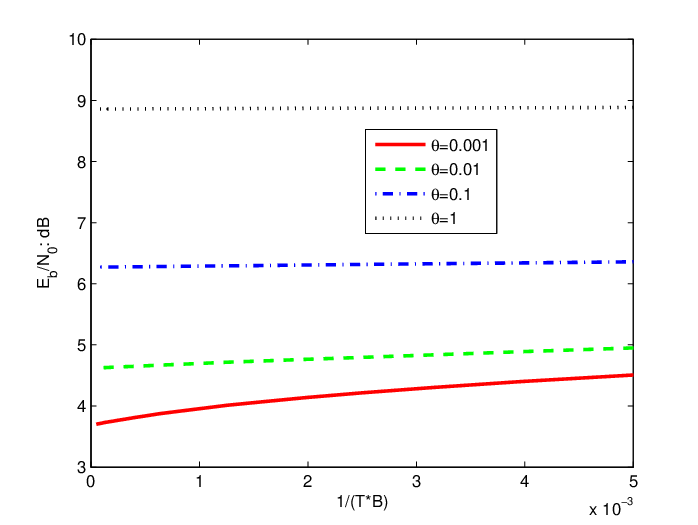
Next, we illustrate the analytical results through numerical computations. Fig. 9 plots the spectral efficiency vs. bit energy for when Hz. We immediately notice a different behavior as and hence the spectral efficiency decreases. As predicted by the result of Theorem 6, the bit energy increases without bound as in all cases. The minimum bit energy is achieved at a nonzero spectral efficiency below which one should avoid operating as it only increases the energy requirements. In Fig. 10, we plot as a function of SNR for different bandwidth levels assuming . We again observe that the minimum bit energy is attained at a nonzero SNR value below which requirements start increasing. Furthermore, we see that as the bandwidth increases, the minimum bit energy tends to decrease and is achieved at a lower SNR level. Finally, we plot in Fig. 11 the minimum bit energy as a function of the bandwidth, . We note that increasing generally decreases when . However, for the cases in which and there exist QoS constraints, there is no improvement as is increased above a certain value.
VII Conclusion
In this paper, we have considered the effective capacity as a measure of the maximum throughput under statistical QoS constraints, and analyzed the energy efficiency of fixed-rate transmission schemes over fading channels. In particular, we have investigated the spectral efficiency–bit energy tradeoff in the low-power and wideband regimes. We have obtained expressions for the bit energy at zero spectral efficiency and the wideband slope, which provide a linear approximation to the spectral efficiency curve at low SNRs. In the wideband regime, we have shown that the bit energy required at zero spectral efficiency (or equivalently at infinite bandwidth) is the minimum bit energy. We have proven a similar result in the low-power regime for a certain class of fading distributions. Through this analysis, we have quantified the increased energy requirements in the presence of QoS constraints in both wideband and low-power regimes. In the wideband regime, we have noted that the minimum bit energy and wideband slope in general depend on the QoS exponent . As the QoS constraints become more stringent and hence is increased, we have observed in the numerical results that the required minimum bit energy increases. On the other hand, in the low power regime, we have shown for a class of fading distributions that the same minimum bit energy is achieved for all . However, we have seen that the wideband slope decreases as increases, increasing the energy requirements at nonzero spectral efficiency values.
We have also analyzed energy efficiency in a scenario in which the fading coefficients are not known prior to transmission and are estimated imperfectly by the receiver with the aid of training symbols. We have identified the optimal fraction of power allocated to training and shown that this optimal fraction do not depend on the QoS exponent and the transmission rate. In this scenario, we have further shown that the bit energy requirements grow without bound in the low-power regime as SNR vanishes. This result shows that the minimum bit energy is attained at a certain SNR value, operating below which should be avoided.
References
- [1] S. Verd, “Spectral efficiency in the wideband regime,” IEEE Trans. Inform. Theory, vol.48, no.6 pp.1319-1343. Jun. 2002.
- [2] A. Ephremides and B. Hajek, “Information theory and communication networks: An unconsummated union,” IEEE Trans. Inform. Theory, vol. 44, pp. 2416-2434, Oct. 1998.
- [3] D. Wu and R. Negi “Effective capacity: a wireless link model for support of quality of service,” IEEE Trans. Wireless Commun., vol.2,no. 4, pp.630-643. July 2003
- [4] D. Wu and R. Negi,“Downlink scheduling in a cellular network for quality-of-service assurance, IEEE Trans. Veh. Technol., vol.53, no.5, pp. 1547-1557, Sep., 2004.
- [5] D. Wu and R. Negi, “Utilizing multiuser diversity for efficient support of quality of service over a fading channel, IEEE Trans. Veh. Technol., vol.49, pp. 1073-1096, May 2003.
- [6] J. Tang and X. Zhang, “Quality-of-service driven power and rate adaptation over wireless links, IEEE Trans. Wireless Commun., vol. 6, no. 8, pp.3058-3068, Aug. 2007.
- [7] J. Tang and X. Zhang, “Quality-of-service driven power and rate adaptation for multichannel communications over wireless links, IEEE Trans. Wireless Commun., vol. 6, no. 12, pp.4349-4360, Dec. 2007.
- [8] J. Tang and X. Zhang, “Cross-layer modeling for quality of service guarantees over wireless links, IEEE Trans. Wireless Commun., vol. 6, no. 12, pp.4504-4512, Dec. 2007.
- [9] J. Tang and X. Zhang, “Cross-layer-model based adaptive resource allocation for statistical QoS guarantees in mobile wireless networks, IEEE Trans. Wireless Commun., vol. 7, pp.2318-2328, June 2008.
- [10] L. Liu, P. Parag, J. Tang, W.-Y. Chen and J.-F. Chamberland, “Resource allocation and quality of service evaluation for wireless communication systems using fluid models,” IEEE Trans. Inform. Theory, vol. 53, no. 5, pp. 1767-1777, May 2007
- [11] L. Liu, P. Parag, and J.-F. Chamberland, “Quality of service analysis for wireless user-cooperation networks,” IEEE Trans. Inform. Theory, vol. 53, no. 10, pp. 3833-3842, Oct. 2007
- [12] L. Liu, and J.-F. Chamberland, “On the effective capacities of multiple-antenna Gaussian channels,” IEEE International Symposium on Information Theory, Toronto, 2008.
- [13] M.C. Gursoy, D. Qiao, and S. Velipasalar, “Analysis of energy efficiency in fading channel under QoS constrains,” submitted to the IEEE Trans. Wireless Commun., 2007; conference version to appear at the IEEE Global Communications Conference (GLOBECOM), Dec. 2008.
- [14] C.-S. Chang, “Stability, queue length, and delay of deterministic and stochastic queuing networks,” IEEE Trans. Auto. Control, vol. 39, no. 5, pp. 913-931, May 1994
- [15] C.-S. Chang, Performance Guarantees in Communication Networks, New York: Springer, 1995
- [16] P. Sadeghi and P. Rapajic, “Capacity analysis for finite-state Markov mapping of flat-fading channels,” IEEE Trans. Commun. vol. 53, pp. 833-840, May 2005.
- [17] L. Tong, B. M. Sadler, and M. Dong, “Pilot-assisted wireless transmission,” IEEE Signal Processing Mag., pp. 12-25, Nov. 2004.
- [18] B. Hassibi and B. M. Hochwald, “How much training is needed in multiple-antenna wireless links”, IEEE Trans. Inform. Theory, vol. 49, pp. 951-963, Apr. 2003.
- [19] M. C. Gursoy, “On the capacity and energy efficiency of training-based transmissions over fading channels,” submitted for publication. Available online at http://arxiv.org/abs/0712.3277.
- [20] A. Lapidoth and S. Shamai (Shitz), “Fading channels: How perfect need ’perfect side information’ be?,” IEEE Trans. Inform. Theory, vol. 48, pp. 1118-1134, May 2002.
- [21] A. Goldsmith, Wireless Communications, 1st ed. Cambridge University Press, 2005.
- [22] Tim Szigeti and Christina Hattingh, End-to-End QoS Network Design: Quality of Service in LANs, WANs, and VPNs, Cisco Press, 2004.
- [23] M. H. Protter, C. B. Morrey, and C. B. Morrey, Jr., A First Course in Real Analysis, 2nd ed., Springer, 1991.
- [24] G. R. Grimmett and D. R. Stirzaker, Probability and Random Processes, 2nd ed. Oxford University Press, 1998.
- [25] I. S. Gradshteyn and I. M. Ryzhik, Table of Integrals, Series, and Products, Academic Press, 2000.
-A Proof of Theorem 4
We consider the following class of Gamma density functions:
| (71) |
where is an integer, and is the Gamma function. Note that for positive integer , . For the above type of density functions, the complementary cumulative distribution function is given by [25, Sec. 8.35]
| (72) |
where is the incomplete Gamma function. Note that is a monotonically decreasing function of .
Next, we consider the function
| (73) |
It can be immediately found that the derivative of with respect to is , from which we conclude that is a monotonically increasing function for and a monotonically decreasing function for . Clearly, achieves its maximum at . Next, we show for all that
| (74) | ||||
| (75) | ||||
| (76) | ||||
| (77) | ||||
| (78) | ||||
| (79) |
Above, (76) is obtained by writing . (77) follows after rearranging the terms. (78) is obtained by noting that for , and therefore . Finally, (79) can easily be verified by applying repetitively the same steps as in (76) – (78) to the other terms in the summation .
(79) shows that after reaching its maximum at , the function is always greater than and hence the two never intersect for . Note that, for , is a monotonically increasing function. Moreover, . On the other hand, is always a monotonically decreasing function of . Note also that at , . Using these facts, we immediately conclude that the function and intersect only once in the interval . Therefore, has a unique solution for when Gamma densities in the form given in (71) are considered.