Modelling solar-like variability for the detection of Earth-like planetary transits
Abstract
Aims. As an extension of a previous work, we present a comparison of four methods of filtering solar-like variability to increase the efficiency of detection of Earth-like planetary transits by means of box-shaped transit finder algorithms. Two of these filtering methods are the harmonic fitting method and the iterative non-linear filter that, coupled respectively with the Box Least-Square (BLS) and Box Maximum-Likelihood algorithms, demonstrated the best performance during the first detection blind test organized inside the CoRoT consortium. The third method, the 3-spot model, is a simplified physical model of Sun-like variability and the fourth is a simple sliding boxcar filter.
Methods. We apply a Monte Carlo approach by simulating a large number of 150-day light curves (as for CoRoT long runs) for different planetary radii, orbital periods, epochs of the first transit and standard deviations of the photon shot noise. Stellar variability is given by the Total Solar Irradiance variations as observed close to the maximum of solar cycle 23. After filtering solar variability, transits are searched for by means of the BLS algorithm.
Results. We find that the iterative non-linear filter is the best method to filter light curves of solar-like stars when a suitable window can be chosen. As the performance of this filter depends critically on the length of its window, we point out that the window must be as long as possible, according to the magnetic activity level of the star. We show an automatic method to choose the extension of the filter window from the power spectrum of the light curves.
Conclusions. The iterative non-linear filter, when used with a suitable choice of its window, has a better performance than more complicated and computationally intensive methods of fitting solar-like variability, like the 200-harmonic fitting or the 3-spot model.
Key Words.
planetary systems – methods: data analysis – techniques: photometric – stars: activity – stars: late-type1 Introduction
To date more than 50 transiting planets over about 300 known extrasolar planets have been discovered11 1 See http://exoplanet.eu/. They are the most interesting to study since transits remove the degeneracy between orbital inclination and amplitude of the radial velocity curve providing us with information on planetary masses and radii. Only for transiting planets it is possible to develop accurate models of their internal structures, study their atmospheres through transmission spectroscopy or infrared emission and detect possible spin-orbit misalignments by measuring the Rossiter-McLaughlin effect.
The new frontier is the search for transiting terrestrial planets. Very recently four super-Earths have been discovered, three of them by means of the radial velocity technique (Mayor et al., 2008) and one by microlensing (Bennett et al., 2008). The latter is a Earth-mass planet and is probably the lowest mass exoplanet found to date, apart from planets around pulsars (Wolszczan & Frail, 1992; Wolszczan, 1994). To detect the transits of terrestrial planets we need to go to space since the photometric precision from the ground is limited to the millimagnitude level because of the scintillation effects produced by the Earth’s atmosphere. The CoRoT space mission, currently operating, can reach the photometric precision to detect transits of Earth-size planets in short period orbits around solar-like stars (Baglin, 2003; Bordé et al., 2003). The Kepler space mission, whose launch is planned in spring 2009, has been specifically designed to find also Earthly twins, i.e., Earth-size planets in Earth-like orbits, transiting solar-type stars (Borucki et al., 2004).
One common approach to searching for planetary transits in light curves of main-sequence late-type stars requires two main steps: first, the filtering of stellar variability to remove distortions produced by the presence of photospheric cool spots and bright faculae, whose visibility is modulated by stellar rotation; secondly, the search for transits in the filtered light curve by means of suitable detection algorithms. The intrinsic stellar variability represents the main source of astrophysical noise in the detection of transits of terrestrial planets even in relatively inactive stars (Defaÿ et al., 2001; Jenkins, 2002; Aigrain & Irwin, 2004; Aigrain et al., 2004, cf., e.g., ).
Several methods to reduce the impact of solar-like variability on the detection of planetary transits have been developed (Defaÿ et al., 2001; Jenkins et al., 2002; Carpano et al., 2003; Aigrain & Irwin, 2004; Moutou et al., 2005; Regulo et al., 2007, see e.g.). Some of them were tested on simulated light curves during the first CoRoT blind test carried out by Moutou et al. (2005). The best performance in terms of reduction of missed detections and false alarms was achieved by team 3 who made use of a linear combination of 200 harmonic functions to filter stellar variability and the Box-fitting Least Square (BLS) algorithm by Kovács et al. (2002) to search for transits in the filtered light curves. Team 5 got the second best performance using the iterative non-linear filter by Aigrain & Irwin (2004) in combination with the Box Maximum Likelihood transit finder algorithm (see Aigrain & Irwin 2004, Sect. 2).
In a recent paper, Bonomo & Lanza (2008) proposed a different method to treat stellar variability, called the 3-spot model, based on the rotational modulation of the flux produced by three point-like active regions (Lanza et al., 2003; Lanza et al., 2007). By analysing a large number of simulated light curves with photon noise, Sun-like variability and planetary transits, they compared its performance with that of the 200-harmonic fitting using the same transit detection algorithm (BLS), to search for transits after the filtering process. They found that the 3-spot model has a better performance than the 200-harmonic fitting when the standard deviation of the noise is 2–4 times larger than the central depth of the transits. On the other hand, the 200-harmonic fitting reduces more efficiently the impact of stellar variability when the standard deviation of the noise is comparable to the transit depth. Bonomo & Lanza (2008) showed that the poor performance of the 200-harmonic fitting in the former case is due to the use of orthogonal functions to fit stellar variability, which makes it significantly affected by the Gibbs phenomenon (Morse & Feshbach, 1954). This latter reduces the depth of the transits in the filtered light curves thus lowering the efficiency of detection in the presence of noise (see Bonomo & Lanza 2008, Sect.5).
The Gibbs phenomenon also affects other filtering methods proposed to reduce the impact of stellar microvariability, such as, e.g., those of Carpano et al. (2003), or the Wiener-like discrete filters by Aigrain & Irwin (2004). Wavelet-based methods (Jenkins, 2002; Regulo et al., 2007, e.g., ) may be useful to overcome the problems related to the Gibbs phenomenon, given the non-orthogonal nature of their basis functions, but they are negatively affected by gaps in the time series. On the other hand, the iterative non-linear filter proposed by Aigrain & Irwin (2004) is practically insensitive to gaps or irregular sampling and does not make use of orthogonal functions. Therefore, in the present paper, we extend our comparison to it and to another simple sliding boxcar filter which has been recently applied by, e.g., Bordé et al. (2003) and Carpano & Fridlund (2008).
2 Filtering methods
A brief description of the filtering methods whose performance will be compared is as follows:
- a)
3-spot model (Lanza et al., 2003; Lanza et al., 2007): it is a simplified physical model of solar-like variability based on the rotational modulation of the flux produced by three active regions, containing both cool spots and warm faculae, plus a uniform background to account for uniformly distributed active regions. In the case of the Sun, the model accounts for the flux variability up to a time scale of 14 days, after which the positions and areas of the three regions and the uniform background have to be changed (for further details see Bonomo & Lanza 2008, Sect.3.1);
- b)
200-harmonic fitting (Moutou et al. 2005, team 3): it fits stellar variability by means of a linear combination of 200 harmonic functions whose frequencies are multiples of the fundamental frequency , where is the whole duration of the time series, i.e., days in the case of the CoRoT mission (for further details see Bonomo & Lanza 2008, Sect.3.2);
- c)
Sliding boxcar filter (hereinafter SBC filter): it is based on a continuum computed by means of a running average of the data with a boxcar window of fixed duration, i.e., each point of the original light curve is replaced by the arithmetic mean of the data points falling within a boxcar window centered at that point. Since at the beginning and the end of the light curve there are not enough data points within the window to compute the continuum, the light curve is extended by mirroring the initial and the last data (edge reflection). The continuum computed according to these prescriptions is then subtracted from the original light curve and the residuals are analysed to detect transits;
- d)
Iterative non-linear filter (hereinafter INL filter; Aigrain & Irwin 2004; Moutou et al. 2005, team 5): it considers a sliding boxcar window of fixed duration and computes an initial continuum by replacing each point of the original light curve with the median of the data within the boxcar window centered at that point (the edges of the light curve are dealt with the technique of edge reflection as in the case of the SBC filter). It computes the residuals between the original light curve and the continuum and estimates their standard deviation from the Median Absolute Deviation (MAD) as =1.4826 MAD. In the residual time series, the points whose absolute deviation is are flagged, and the continuum is recomputed from the original time series without the flagged points, iterating the process up to convergence. The final continuum is then subtracted from the original light curve.
3 Light curve simulation and analysis
We apply a Monte Carlo approach by simulating a large number of light curves with sampling of 1 hour and duration 150 days (the extension of the CoRoT long runs) for different values of planetary radius ranging from 1.0 to 2.0 Earth radii, orbital period between 5 and 50 days, and standard deviation of the photon shot noise from 100 to 1000 parts per millions (ppm). A noise level =100 ppm is obtained for a star of magnitude 12 observed in white light by CoRoT with 1 hr integration time, while =200, 300 and 1000 ppm correspond to stars of 13, 14 and 16, respectively, observed with the same instrument and 1 hr integration time22 2 http://corotsol.obspm.fr/web-instrum/payload.param/index.html. The phase of the first transit is taken from a uniform random distribution. The star is assumed to have the solar radius and mass. We add stellar variability, assumed in all cases to be given by the Total Solar Irradiance variations as observed close to the maximum of solar cycle 23 (e.g., Fröhlich & Lean 2004). To reduce systematic effects associated with a particular realization of the TSI, we select a time series of the TSI of duration 150 days with a random initial epoch between January 1st and January 20th 2001. For each set of planetary parameters and noise level, we simulate 100 light curves with different noise and activity realizations, for a total of 8000 light curves. For further details, see Bonomo & Lanza (2008), Sect. 2.
After filtering solar variability with the four different filtering methods, transits are searched for in the filtered light curves by means of the BLS algorithm (Kovács et al. 2002). See Bonomo & Lanza (2008), Sect. 3.3, for the choice of the algorithm’s free parameter ranges and steps. The period search is carried out between 1 and 150 days so that also single transit events are searched for. For this reason, as a detection statistic, we prefer to use the signal-to-noise ratio of a putative transit (see Kovács et al. 2002, Eq. 11) instead of the Signal Detection Efficiency (hereinafter SDE, see Kovács et al. 2002, Eq. 6) used, e.g., by team 3 for the analysis of the first CoRoT blind test light curves (see Sect. 4.3 for a discussion about the difference between these statistics).
Transitless light curves obtained by combining solar irradiance variations with random sequences of white Gaussian noise are analysed in the same way to establish the transit detection threshold for each filtering method. For our analysis, this threshold is chosen in such a way as to have a false alarm rate of 1% in a set of one hundred light curves.
The large computational load of our experiment is managed by running our analyses on the grid infrastructure of the project PI2S2, allowing us to use up to about 2000 CPUs in parallel (e.g., Becciani 2007). The CPU time for filtering stellar microvariability with the four methods is on the average about 16 minutes, while about 3 days of elapsed time have been necessary to analyse the complete set of 8000 light curves.
4 Results
After a series of tests, we have found that an appropriate window both for the SBC and the INL filters is 2 days when we adopt the TSI time series as a proxy for the variability of solar-like stars. Specifically, we found that the shorter the window, the greater the reduction of the transit depth and the worse the detection performance by means of the BLS algorithm. On the other hand, with a window longer than 2 days, spurious transit-like features might appear in the residuals, owing to a worse filtering of the variability.
A sample of our results is provided in Fig. 1 that shows the distributions of the values of , the signal-to-noise ratio of a transit detection, obtained by analysing light curves with transits of a 1.75 R⊕ planet and white Gaussian noise of 200 ppm. Each set is characterized by a different orbital period of the planet (as labelled). In the left panels, the red and blue vertical dot-dashed lines indicate the 1 percent false-alarm threshold for the 200-harmonic fitting and the 3-spot model, respectively. They are derived from the analysis of the transitless light curves under the requisite that the frequency of false alarms be . Red solid histograms show the statistics of light curves where the period was correctly identified by the BLS, within days, after applying the 200-harmonic method; blue solid histograms show those after applying the 3-spot method. Dashed histograms refer to the statistics of light curves where the period was incorrectly identified by the BLS after the filtering process, with the same color coding. These latter increase with increasing orbital period, because the number of transits in the light curve becomes smaller giving a lower signal-to-noise ratio. Right panels show the distributions of the values obtained analysing the same simulated light curves after applying the 3-spot model (blue histograms) and the INL filter (green histograms). In this case, the dot-dashed vertical lines indicating the false alarm thresholds overlap.
Table 1 reports the frequencies of detections and false alarms obtained for different values of planetary radius, orbital period and noise level, omitting the entries corresponding to null detections, with the exception of the first ones. As a detection, we count each case with a period correctly identified by the BLS and a corresponding value greater than the detection threshold. False alarms are those cases where the values are above the detection threshold but the period is not correctly found. In the first column of Table 1, we list the planetary radius ; in the second, the standard deviation of the Gaussian photon shot noise ; in the third, the orbital period ; from the fourth to the seventh column, the frequency of detections obtained with the 200-harmonic fitting , the 3-spot model , the INL filter and the SBC filter , respectively; from the eighth to the eleventh column, the frequency of false alarms , , and , produced by the four filtering methods.
We report below on the performance of the different filters, according to the different values of the standard deviation of the photon shot noise.


4.1 100 ppm
Detection performance: The filtering methods that achieve the best performance are the INL filter and the 200-harmonic fitting. In most cases they give comparable results, although in some instances the INL filter has a slightly better performance (see Table 1), owing to the fact that the 200-harmonic fitting is affected by the Gibbs phenomenon (Morse & Feshbach 1954, Bonomo & Lanza 2008, Sect. 5).
The method that has the worst performance is the SBC filter because it gives rise to the greatest number of false alarms when applied to the transitless light curves. Therefore, we are forced to increase the transit detection threshold to push the false alarm rate below the 1% level. Inspecting the light curves without transits that give rise to false detections, we find that they are affected by the presence of a positive spike close to the beginning of their 150-day TSI subsets. This spike is probably due to an instrumental effect of the VIRGO radiometers. When we apply the technique of edge reflection to deal with the first sections of these light curves (i.e., the first 24 data points), the computation of the continuum by means of a running average of the data is significantly affected by that spike giving rise to a transit-like feature at the beginning of the residual time series. The BLS algorithm detects this transit-like feature, possibly phased with some other residual dips, as a transit and gives rise to a false alarm. We could overcome such a problem by making all the points within the first day equal to zero, i.e., without using the edge reflection technique to deal with the beginning of the light curves. In this case, however, we could loose some transits whose initial phase is close to zero, again having a deterioration of the detection performance.
Although, in our particular case, the technique of edge reflection clearly amplifies the above-mentioned effect, generally speaking, a variability filter based on the computation of the continuum by means of a running average is certainly more sensitive to the presence of outliers than a median filter. This makes a median filter less affected by false alarms.
False alarms: Once the detection threshold was established by the analysis of the transitless light curves, the percentage of false alarms given by the four filtering methods in the analysis of the light curves with transits is usually below 2%. Only the 200-harmonic fitting, in some cases, gives rise to a 4% false alarms (see Table 1).
4.2 200 ppm
Detection performance: The method with the best performance proves to be the INL filter when we use an appropriate window of 2 days. It has a performance comparable with that of the 3-spot model in most of the cases, even better in some instances (see Fig. 1 and Table 1). On the other hand, the 200-harmonic fitting has the worst performance owing to the Gibbs phenomenon (see Fig. 1 and Table 1). Finally, the SBC filter has a performance better than the 200-harmonic fitting but slightly worse than the 3-spot model and the INL filter for the same reason explained above, i.e., the transit detection threshold (or threshold) must be increased with respect to those of the other filtering methods to maintain the false alarm rate below 1% in the transitless light curves.
False alarms: Once the detection threshold was established by the analysis of the transitless light curves, the percentage of false alarms given by the four filtering methods in the light curves with transits is usually below 3%. None of the four filters produces significantly more false alarms than the others (see Table 1).
| () | (ppm) | (d) | ||||||||
|---|---|---|---|---|---|---|---|---|---|---|
| 1.0 | 100 | 5.0 | 0.93 | 0.36 | 0.91 | 0.14 | 0.00 | 0.01 | 0.00 | 0.00 |
| 10.0 | 0.31 | 0.03 | 0.31 | 0.00 | 0.04 | 0.00 | 0.02 | 0.00 | ||
| 25.0 | 0.01 | 0.00 | 0.01 | 0.00 | 0.01 | 0.00 | 0.00 | 0.01 | ||
| 50.0 | 0.00 | 0.00 | 0.00 | 0.00 | 0.01 | 0.01 | 0.00 | 0.00 | ||
| 1.0 | 200 | 5.0 | 0.02 | 0.06 | 0.08 | 0.06 | 0.01 | 0.01 | 0.01 | 0.01 |
| 10.0 | 0.00 | 0.00 | 0.00 | 0.00 | 0.00 | 0.00 | 0.00 | 0.01 | ||
| 1.25 | 100 | 5.0 | 1.00 | 1.00 | 1.00 | 0.98 | 0.00 | 0.00 | 0.00 | 0.00 |
| 10.0 | 0.98 | 0.77 | 0.97 | 0.43 | 0.01 | 0.01 | 0.00 | 0.01 | ||
| 25.0 | 0.34 | 0.01 | 0.46 | 0.00 | 0.00 | 0.00 | 0.02 | 0.01 | ||
| 50.0 | 0.01 | 0.01 | 0.05 | 0.00 | 0.04 | 0.01 | 0.01 | 0.00 | ||
| 1.25 | 200 | 5.0 | 0.46 | 0.61 | 0.62 | 0.50 | 0.00 | 0.00 | 0.01 | 0.03 |
| 10.0 | 0.06 | 0.12 | 0.19 | 0.10 | 0.01 | 0.00 | 0.02 | 0.01 | ||
| 25.0 | 0.00 | 0.02 | 0.01 | 0.02 | 0.03 | 0.00 | 0.00 | 0.00 | ||
| 50.0 | 0.00 | 0.00 | 0.00 | 0.00 | 0.00 | 0.00 | 0.00 | 0.00 | ||
| 1.25 | 300 | 5.0 | 0.02 | 0.06 | 0.06 | 0.01 | 0.02 | 0.00 | 0.00 | 0.01 |
| 10.0 | 0.00 | 0.01 | 0.00 | 0.00 | 0.01 | 0.01 | 0.00 | 0.00 | ||
| 25.0 | 0.00 | 0.00 | 0.00 | 0.00 | 0.01 | 0.01 | 0.01 | 0.00 | ||
| 1.5 | 100 | 5.0 | 1.00 | 1.00 | 1.00 | 1.00 | 0.00 | 0.00 | 0.00 | 0.00 |
| 10.0 | 1.00 | 1.00 | 1.00 | 1.00 | 0.00 | 0.00 | 0.00 | 0.00 | ||
| 25.0 | 0.97 | 0.88 | 0.99 | 0.66 | 0.00 | 0.00 | 0.01 | 0.03 | ||
| 50.0 | 0.16 | 0.06 | 0.54 | 0.03 | 0.04 | 0.00 | 0.02 | 0.01 | ||
| 1.5 | 200 | 5.0 | 0.99 | 1.00 | 1.00 | 0.99 | 0.01 | 0.00 | 0.00 | 0.01 |
| 10.0 | 0.62 | 0.85 | 0.85 | 0.84 | 0.02 | 0.00 | 0.01 | 0.01 | ||
| 25.0 | 0.00 | 0.10 | 0.15 | 0.08 | 0.01 | 0.02 | 0.00 | 0.01 | ||
| 50.0 | 0.00 | 0.01 | 0.01 | 0.00 | 0.00 | 0.01 | 0.03 | 0.01 | ||
| 1.5 | 300 | 5.0 | 0.49 | 0.61 | 0.59 | 0.53 | 0.01 | 0.01 | 0.00 | 0.00 |
| 10.0 | 0.02 | 0.17 | 0.17 | 0.09 | 0.00 | 0.00 | 0.00 | 0.02 | ||
| 25.0 | 0.00 | 0.00 | 0.00 | 0.00 | 0.00 | 0.00 | 0.01 | 0.00 | ||
| 1.75 | 100 | 5.0 | 1.00 | 1.00 | 1.00 | 1.00 | 0.00 | 0.00 | 0.00 | 0.00 |
| 10.0 | 1.00 | 1.00 | 1.00 | 1.00 | 0.00 | 0.00 | 0.00 | 0.00 | ||
| 25.0 | 1.00 | 1.00 | 1.00 | 1.00 | 0.00 | 0.00 | 0.00 | 0.01 | ||
| 50.0 | 0.88 | 0.77 | 0.99 | 0.57 | 0.01 | 0.00 | 0.01 | 0.00 | ||
| 1.75 | 200 | 5.0 | 1.00 | 1.00 | 1.00 | 1.00 | 0.00 | 0.00 | 0.00 | 0.00 |
| 10.0 | 0.97 | 0.99 | 0.99 | 0.99 | 0.01 | 0.01 | 0.00 | 0.01 | ||
| 25.0 | 0.27 | 0.60 | 0.72 | 0.59 | 0.01 | 0.00 | 0.00 | 0.01 | ||
| 50.0 | 0.00 | 0.10 | 0.14 | 0.07 | 0.00 | 0.02 | 0.02 | 0.01 | ||
| 1.75 | 300 | 5.0 | 0.95 | 0.99 | 1.00 | 0.99 | 0.02 | 0.00 | 0.01 | 0.02 |
| 10.0 | 0.36 | 0.58 | 0.61 | 0.48 | 0.00 | 0.03 | 0.03 | 0.01 | ||
| 25.0 | 0.00 | 0.06 | 0.09 | 0.03 | 0.01 | 0.00 | 0.00 | 0.02 | ||
| 50.0 | 0.00 | 0.00 | 0.00 | 0.00 | 0.01 | 0.00 | 0.01 | 0.04 | ||
| 2.0 | 100 | 5.0 | 1.00 | 1.00 | 1.00 | 1.00 | 0.00 | 0.00 | 0.00 | 0.00 |
| 10.0 | 1.00 | 1.00 | 1.00 | 1.00 | 0.00 | 0.00 | 0.00 | 0.00 | ||
| 25.0 | 1.00 | 1.00 | 1.00 | 1.00 | 0.00 | 0.00 | 0.00 | 0.00 | ||
| 50.0 | 1.00 | 1.00 | 1.00 | 0.99 | 0.00 | 0.00 | 0.01 | 0.01 | ||
| 2.0 | 200 | 5.0 | 1.00 | 1.00 | 1.00 | 1.00 | 0.00 | 0.00 | 0.00 | 0.00 |
| 10.0 | 1.00 | 1.00 | 1.00 | 1.00 | 0.00 | 0.00 | 0.00 | 0.00 | ||
| 25.0 | 0.92 | 0.99 | 0.99 | 0.99 | 0.00 | 0.00 | 0.00 | 0.00 | ||
| 50.0 | 0.09 | 0.57 | 0.73 | 0.58 | 0.02 | 0.02 | 0.00 | 0.01 | ||
| 2.0 | 300 | 5.0 | 1.00 | 1.00 | 1.00 | 1.00 | 0.00 | 0.00 | 0.00 | 0.00 |
| 10.0 | 0.97 | 1.00 | 1.00 | 0.99 | 0.01 | 0.00 | 0.00 | 0.00 | ||
| 25.0 | 0.08 | 0.42 | 0.47 | 0.36 | 0.02 | 0.00 | 0.01 | 0.01 | ||
| 50.0 | 0.00 | 0.01 | 0.02 | 0.02 | 0.00 | 0.02 | 0.01 | 0.01 | ||
| 2.0 | 1000 | 5.0 | 0.00 | 0.01 | 0.01 | 0.00 | 0.01 | 0.01 | 0.00 | 0.02 |
| 10.0 | 0.00 | 0.00 | 0.00 | 0.00 | 0.01 | 0.01 | 0.00 | 0.01 |
4.3 versus SDE statistics
Using the SDE statistic instead of the statistic, the results in terms of detection rates and false alarm percentages obtained by the 200-harmonic fitting, the 3-spot model and the INL filter are very similar in the cases when ppm, that is for most of our simulations. Specifically, the detection rates differ from those reported in Table 1 by no more than 2-3%. Only the SBC filter, in a few cases, shows an improvement of the detection rate of about 5-6% but its performance is never better than that of the INL filter.
Different results are obtained in the cases where ppm when the SDE statistic is adopted: the detection rates of the 3-spot model and the SBC filter show a significant improvement reaching those of the 200-harmonic fitting with false alarm rates below 2%. The reason of such a behaviour is as follows. The statistic is much more sensitive to single transit events than the SDE statistic, especially for low levels of noise. This is due to the fact that, if there is a single transit event, the BLS algorithm detects it several times while trying different orbital periods, which gives rise to a great dispersion of the Signal Residue in the BLS spectrum (see Kovács et al. 2002, Eq. 5) and therefore to a decrease of the SDE statistic that is inversely proportional to the standard deviation of the Signal Residue (see Kovács et al. 2002, Eq. 6). The statistic, on the other hand, does not suffer from this problem and therefore it is more suitable to search for monotransits. We prefer to use it since in our analysis the period search is carried out between 1 and 150 days. However, for the same reason as above, the statistic is also more sensitive to sporadic transit-like features produced by the filtering of the stellar variability with the SBC filter and the 3-spot model (see Sect. 4.1 and Bonomo & Lanza 2008, Sect. 5). When we apply the statistic to cases with ppm, those features force us to increase the detection thresholds in order to have a false alarm rate below the 1% level in the transitless light curves. Such an increase leads to a worse detection performance in the light curves with transits. From this point of view, the SDE statistic seems to be more robust against false alarms for low noise levels ( ppm). Nevertheless, the detection of single transit events is sometimes important. For instance, the CoRoT alarm mode searches for transits while data are arriving and, when it detects a single transit, it allows to change the time sampling of the light curve to seek transit timing variations (Bordé et al., 2003). In this case, the SDE statistic is not appropriate and the statistic is certainly more suitable.
5 Discussion
From the above mentioned results we conclude that team 3 of the CoRoT Blind Test achieved the best performance mostly thanks to the use of the BLS, one of the most powerful transit detection algorithms, rather than by virtue of their detrending method. However, the 200-harmonic fitting has the advantage of being fully automatic, in particular it is independent of the activity level of the star thanks to the high number of free parameters (=401). On the other hand, the other filtering techniques need to adjust some of their parameters according to the activity level of the star. In particular, to fit the light curve of a star more active than the Sun, the 3-spot method requires to change the rotation period, the limb-darkening, the maximum spot area or the contrast of spots, and the duration of the individually fitted time intervals (cf. Lanza et al. 2003 for details). In the case of the INL and the SBC filters, the extension of the window should be reduced for stars more active than the Sun, otherwise some oscillations or transit-like features will appear in the residuals owing to a bad filtering of the variability.
We could make the INL and SBC filters automatic by introducing a method to choose the extension of the filter window according to the magnetic activity level of the star. We propose to use a method similar to that suggested by Regulo et al. (2007), based on the computation of the power spectrum of the data to find the frequency intervals where most of the power is concentrated and choose automatically the filter window corresponding to the frequency where the power spectral density goes below a fixed threshold. The power spectrum of the Total Solar Irradiance can be modelled as a sum of power laws, each of which corresponds to a separate class of physical phenomena, taking place on different characteristic time scales (Harvey, 1985; Aigrain et al., 2004). For our purpose, it is sufficient to perform a best-fit of the power spectrum of a light curve by means of a single power law, corresponding to the evolution and rotational modulation of active regions, i.e.,
| (1) |
where is the frequency, , and represent the amplitude, the characteristic time scale and the slope of the power law, respectively (see Fig. 2). The inverse of the frequency such that
| (2) |
gives the window extension to use.

An alternative to such a method would be using a very short window extension, i.e., only two or three times the transit duration, to filter the light curves of both quiet and active stars, as team 5 did for the CoRoT BT1. However, a very short window, when not necessary, as in the case of quiet solar-like stars, is not advisable because it gives rise to a reduction of the transit depth in the filtered light curve (see Fig. 3) and therefore to a worse detection performance when the BLS algorithm is applied.
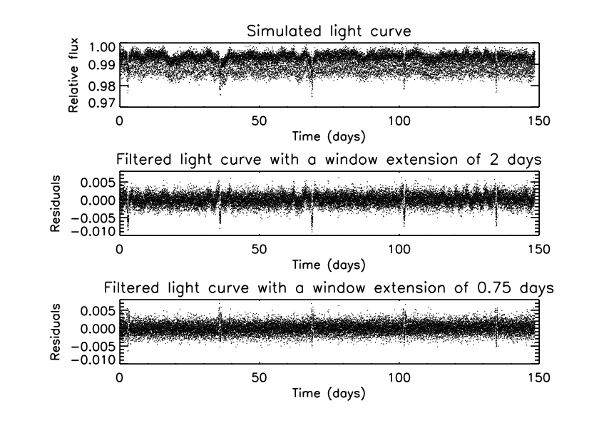
To show the deterioration of the detection performance with the reduction of the window extension for the INL and the SBC filters, we consider the simulated light curves for a planet of =1.75 R⊕ and analyse them using four different window extensions of 12, 24, 36 and 48 hours in the same way as explained in Sect. 3. For each window extension, we redetermine appropriate transit detection thresholds by analysing the transitless light curves. The results are presented in Table 2 where, in the first column, we list the window extension ; in the second, the standard deviation of the photon noise; in the third, the simulated orbital period of the planet; in the fourth and fifth column, the frequency of transit detections and obtained respectively with the INL and the SBC filters; in the sixth and seventh column, the false alarm rates and produced by both methods.
| (h) | (ppm) | (d) | ||||
|---|---|---|---|---|---|---|
| 12 | 100 | 5.0 | 1.00 | 1.00 | 0.00 | 0.00 |
| 10.0 | 1.00 | 1.00 | 0.00 | 0.00 | ||
| 25.0 | 1.00 | 1.00 | 0.01 | 0.00 | ||
| 50.0 | 0.09 | 0.21 | 0.03 | 0.00 | ||
| 12 | 200 | 5.0 | 1.00 | 1.00 | 0.00 | 0.00 |
| 10.0 | 0.89 | 0.94 | 0.01 | 0.01 | ||
| 25.0 | 0.06 | 0.08 | 0.02 | 0.00 | ||
| 50.0 | 0.00 | 0.00 | 0.00 | 0.01 | ||
| 12 | 300 | 5.0 | 0.86 | 0.92 | 0.03 | 0.03 |
| 10.0 | 0.19 | 0.26 | 0.03 | 0.03 | ||
| 25.0 | 0.00 | 0.00 | 0.02 | 0.02 | ||
| 50.0 | 0.00 | 0.00 | 0.02 | 0.00 | ||
| 12 | 1000 | 5.0 | 0.00 | 0.00 | 0.01 | 0.01 |
| 24 | 100 | 5.0 | 1.00 | 1.00 | 0.00 | 0.00 |
| 10.0 | 1.00 | 1.00 | 0.00 | 0.00 | ||
| 25.0 | 1.00 | 0.99 | 0.00 | 0.01 | ||
| 50.0 | 0.98 | 0.98 | 0.02 | 0.00 | ||
| 24 | 200 | 5.0 | 1.00 | 1.00 | 0.00 | 0.00 |
| 10.0 | 0.98 | 0.99 | 0.01 | 0.01 | ||
| 25.0 | 0.47 | 0.41 | 0.01 | 0.00 | ||
| 50.0 | 0.06 | 0.01 | 0.01 | 0.00 | ||
| 24 | 300 | 5.0 | 0.96 | 0.97 | 0.01 | 0.02 |
| 10.0 | 0.44 | 0.50 | 0.02 | 0.00 | ||
| 25.0 | 0.03 | 0.03 | 0.01 | 0.02 | ||
| 50.0 | 0.00 | 0.00 | 0.00 | 0.02 | ||
| 24 | 1000 | 5.0 | 0.00 | 0.00 | 0.01 | 0.01 |
| (h) | (ppm) | (d) | ||||
|---|---|---|---|---|---|---|
| 36 | 100 | 5.0 | 1.00 | 1.00 | 0.00 | 0.00 |
| 10.0 | 1.00 | 1.00 | 0.00 | 0.00 | ||
| 25.0 | 1.00 | 0.98 | 0.00 | 0.02 | ||
| 50.0 | 0.99 | 0.80 | 0.01 | 0.01 | ||
| 36 | 200 | 5.0 | 1.00 | 1.00 | 0.00 | 0.00 |
| 10.0 | 0.99 | 0.99 | 0.00 | 0.01 | ||
| 25.0 | 0.71 | 0.46 | 0.01 | 0.00 | ||
| 50.0 | 0.12 | 0.03 | 0.02 | 0.00 | ||
| 36 | 300 | 5.0 | 0.99 | 0.96 | 0.01 | 0.02 |
| 10.0 | 0.57 | 0.43 | 0.02 | 0.00 | ||
| 25.0 | 0.06 | 0.02 | 0.00 | 0.01 | ||
| 50.0 | 0.00 | 0.00 | 0.00 | 0.02 | ||
| 36 | 1000 | 5.0 | 0.00 | 0.00 | 0.00 | 0.01 |
| 48 | 100 | 5.0 | 1.00 | 1.00 | 0.00 | 0.00 |
| 10.0 | 1.00 | 1.00 | 0.00 | 0.00 | ||
| 25.0 | 1.00 | 1.00 | 0.00 | 0.01 | ||
| 50.0 | 0.99 | 0.57 | 0.01 | 0.00 | ||
| 48 | 200 | 5.0 | 1.00 | 1.00 | 0.00 | 0.00 |
| 10.0 | 0.99 | 0.99 | 0.00 | 0.01 | ||
| 25.0 | 0.72 | 0.59 | 0.00 | 0.01 | ||
| 50.0 | 0.14 | 0.07 | 0.02 | 0.01 | ||
| 48 | 300 | 5.0 | 1.00 | 0.99 | 0.01 | 0.02 |
| 10.0 | 0.61 | 0.48 | 0.03 | 0.01 | ||
| 25.0 | 0.09 | 0.03 | 0.00 | 0.02 | ||
| 50.0 | 0.00 | 0.00 | 0.01 | 0.04 | ||
| 48 | 1000 | 5.0 | 0.00 | 0.00 | 0.00 | 0.01 |
Let us consider for example the case with a window of 12 h, =300 ppm and =10 d. In this case the window extension is three times the transit duration. We note that: a) after the INL filtering, the positive detections are 19% versus 61% when a 2 day (48 h) window was applied; b) the positive detections obtained after SBC filtering are 26% versus 48% with a window of 2 days. Therefore, if we used a window extension equal to three times the transit duration for the INL and the SBC filters, the 3-spot model would be the best method (with its 58% positive detections, see Table 1) and even the performance of the 200-harmonic fitting (36% positive detections) would be better than that of the INL and SBC filters.
Similar results are obtained in the case with a window extension of 24 h, =200 ppm and =25 d. In this case the window is four and a half times the transit duration. In the case of the INL filtering, the positive detections decrease from 72% with a window of 2 days to 47% with a 1 day window; regarding the SBC filter, they decrease from 59% to 41%. Once again, the 3-spot model would prove to be the best filtering method (see Table 1).
Note that in some cases (i.e., =300 ppm, =10 d) the performance of the SBC filter does not vary in a monotonic way as a function of the window extension, owing to the effect of the changing detection threshold.
Looking at the results obtained with a 12 h window, we see that the SBC filter is slightly more efficient than the INL filter. This is connected with the fact that, reducing the filter window, we reduce the number of data points from which each value of the continuum is computed. With a fewer data points, the median used by the INL filter is more affected by statistical fluctuations than the arithmetic mean used by the SBC, so the former gives rise to a distribution of the residuals with a greater standard deviation and higher tails than that obtained with the SBC filter. In other words, in the case of a short window with a small number of data points, the continuum is better computed by the SBC filter, giving rise to a better detection performance by means of the BLS.
Although we have pointed out that, with an inappropriate window, the INL filter has a performance worse than the 3-spot model, the latter is computationally much more intensive, being based on a physical model of stellar variability. The time it takes to filter one light curve is 10 min against 3 min with the 200-harmonic fitting and just a few seconds with the INL and the SBC filters. Therefore, the use of the INL filter with a window extension determined according to the magnetic activity level of the star is preferable to the 3-spot model.
6 Conclusions
We have performed extensive numerical experiments to compare the performance of four different variability filters for the detection of Earth-like planetary transits by means of a box-shaped transit finder algorithm. The INL filter has proved to be the best method to filter light curves of quiet solar-like stars when a sufficiently long window can be chosen. We have shown that the choice of the window of the filter is critical since its performance depends significantly on it. We point out that the window must be as long as possible, according to the magnetic activity level of the star. A method to choose the extension of the window, similar to that proposed by Regulo et al. (2007), is shown in Sect. 5. The INL filter, when used with a suitable choice of its window, has a better performance than more complicated and computationally intensive methods of fitting solar-like variability, like the 200-harmonic fitting or the 3-spot model.
Acknowledgements.
The authors are grateful to Dr. R. Alonso for useful discussions and acknowledge an anonymous Referee for valuable comments. They are grateful also to Drs. U. Becciani, A. Costa, A. Grillo, and the system managers of the Trigrid and Cometa Consortia for their technical advice and kind assistance during the implementation and running of the numerical experiments on grid-based high performance computing systems. The availability of unpublished data of the VIRGO Experiment on the cooperative ESA/NASA Mission SoHO from the VIRGO Team through PMOD/WRC, Davos, Switzerland, is gratefully acknowledged. ASB and AFL gratefully acknowledge support from the Italian Space Agency (ASI) under contract ASI/INAF I/015/07/0, work package 3170. Part of this work was carried out during a visit to Exeter by ASB, for which the authors gratefully acknowledge support from grant PP/D001617/1 from the UK Science and Technology Facilities Council. This research has made use of results produced by the PI2S2 Project managed by the Consorzio COMETA, a project co-funded by the Italian Ministero dell’Istruzione, Università e Ricerca (MIUR) within the Piano Operativo Nazionale "Ricerca Scientifica, Sviluppo Tecnologico, Alta Formazione" (PON 2000-2006). More information is available at http://www.pi2s2.it and http://www.consorzio-cometa.it. Active star research and exoplanetary studies at INAF-Catania Astrophysical Observatory and the Department of Physics and Astronomy of Catania University are funded by MIUR (Ministero dell’Istruzione, Università e Ricerca), and by Regione Siciliana, whose financial support is gratefully acknowledged. This research has made use of the ADS-CDS databases, operated at the CDS, Strasbourg, France.References
- Aigrain et al. (2004) Aigrain, S., Favata, F., Gilmore, G. 2004, A&A, 414, 1139
- Aigrain & Irwin (2004) Aigrain, S., Irwin, M. 2004, MNRAS, 350, 331
- Baglin (2003) Baglin, A. 2003, Adv. Sp. Res., 31, 345
- Becciani (2007) Becciani, U. 2007, in Grid-enabled Astrophysics, L. Benacchio, F. Pasian, Eds., Edizioni Polimetrica; p. 179
- Bennett et al. (2008) Bennett, D. P., Bond, I. A., Udalski, A., Sumi, T., Abe, F. et al. 2008, ApJ, in press, (arXiv:0806.0025)
- (2008) Bonomo, A. S., Lanza, A. F. 2008, A&A, 482, 341
- Bordé et al. (2003) Bordé, P., Rouan, D., Léger, A. 2003, A&A, 405, 1137
- Borucki et al. (2004) Borucki, W., Koch, D., Boss, A., et al. 2004, in Second Eddington Workshop: Stellar structure and habitable planet finding, eds. F. Favata, S. Aigrain, & A. Wilson, ESA SP-538, 177
- Carpano et al. (2003) Carpano, S., Aigrain, S., Favata, F. 2003, A&A, 401, 743
- Carpano & Fridlund (2008) Carpano, S. & Fridlund, M. 2008, A&A, 485, 607
- Defaÿ et al. (2001) Defaÿ C., Deleuil, M., Barge, P. 2001, A&A, 365, 330
- Doyle et al. (2000) Doyle, L. R., Deeg, H. J., Kozhevnikov, V. P., Oetiker, B., Martín, E. L., et al. 2000, ApJ, 535, 338
- (2004) Fröhlich, C., Lean, J. 2004, A&ARv, 12, 273
- Harvey (1985) Harvey, J. W. 1985, in ESA Future missions in solar, heliospheric and space plasma physics, eds. E. Rolfe, & B. Battrick, ESA SP-235, 199
- Jenkins (2002) Jenkins, J. M. 2002, ApJ, 575, 493
- Jenkins et al. (2002) Jenkins, J. M., Caldwell, D. A., Borucki, W. J. 2002, ApJ, 564, 495
- Kovács et al. (2002) Kovács, G., Zucker, S., Mazeh, T. 2002, A&A, 391, 369
- Lanza et al. (2003) Lanza, A. F., Rodonò, M., Pagano, I., Barge, P., Llebaria, A. 2003, A&A, 403, 1135
- Lanza et al. (2007) Lanza, A. F., Bonomo, A. S., Rodonò, M. 2007, A&A, 464, 741
- Mayor et al. (2008) Mayor, M., Udry, S., Lovis, C., Pepe, F., Queloz, D., et al. 2008, A&A, submitted (arXiv:0806.4587)
- Morse & Feshbach (1954) Morse, P. M., Feshbach, H. 1954, Methods of Theoretical Physics, McGraw-Hill Book Co. Inc., New York
- Moutou et al. (2005) Moutou, C., Pont, F., Barge, P., Aigran, S., Auvergne, M., et al. 2005, A&A, 437, 355
- Regulo et al. (2007) Regulo, C., Almenara, J. M., Alonso, R., Deeg H., Roca Cortes T. 2007, A&A, 467, 1345
- Wolszczan & Frail (1992) Wolszczan, A., Frail, D. A. 1992, Nature, 335, 145
- Wolszczan (1994) Wolszczan, A., 1994, Science, 264, 538