Bulk spacetimes for cosmological braneworlds with a time-dependent extra dimension

Suman Ghosh and Sayan Kar Note: Electronic address : suman@cts.iitkgp.ernet.in Note: Electronic address : sayan@cts.iitkgp.ernet.in Affiliation: Department of Physics and Centre for Theoretical Studies
Indian Institute of Technology, Kharagpur 721 302, India

Abstract

We explore the possibilities of constructing bulk spacetimes in five dimensions for warped braneworld models with a spatially flat Friedmann-Robertson-Walker (FRW) line element on the 3-brane and with a time-dependent extra dimension. Our first step in this direction involves looking at the status of energy conditions when such a bulk line element is assumed. We check these conditions by analysing the relevant inequalities, for specific functional forms (chosen to satisfy certain desirable features) of the warp factor, the cosmological scale factor and the extra-dimensional scale factor. Subsequently, we aim at obtaining solutions with different types of bulk matter sources. We begin with a general analysis of the solution space of non-singular Randall-Sundrum type bulk models with an exponential warp factor and a chosen equation of state. Thereafter, we focus on three specific bulk sources – the ordinary scalar field, the Brans-Dicke scalar and the dilaton. In each case, we are able to solve the field equations and obtain desirable solutions for which, we once again check the viability of the energy conditions. We also show how one can place branes in the bulk using the junction conditions. The issue of resolution of the bulk singularities which appear in our solutions, using standard methods, is also presented briefly. In summary, we are able to demonstrate, that it is indeed possible to construct viable bulk spacetimes for warped cosmological braneworlds with a time-varying extra dimension and with bulk matter satisfying the energy conditions.

pacs

04.50.-h, 04.20.Jb, 11.10.Kk

I Introduction

Though yet to be seen in experiments, extra dimensions have been around in theoretical constructs for almost a century now. The fact that such a seemingly exotic idea has survived for so long seems to make us feel that there is bound to be some amount of advantage in having them. The advantage stems from several directions. For instance, one may ask – why four dimensions? – a question to which one really does not have an answer. Or, while making models of unification (such as superstrings [1]) one ends up with a need of more dimensions and the subsequent need for compactification. More recently, we have seen how the age-old problem –the hierarchy problem–can be solved (obviously not uniquely) with extra dimensions [2].

The most popular among today’s models is the one we mentioned at the end in the last paragraph– the so-called warped braneworld or Randall-Sundrum (referred henceforth as RS) model. This model assumes a curved spacetime (the bulk) in five dimensions. The four dimensional piece however, depends on the extra dimension, a feature unique for this class of models (different from the usual Kaluza–Klein [3]). Thus, in such a model we have a metric ansatz:

ds^{2}=e^{2f(\sigma)}\left(-dt^{2}+d{\vec{x}}^{2}\right)+r_{c}^{2}d\sigma^{2}

(1)

The $\sigma=constant$ (say $\sigma_{0}$ ) section is a four dimensional Minkowski space scaled by the factor $e^{2f(\sigma=\sigma_{0})}$ .

But such a metric ansatz is toy. This is because the metric on the $\sigma=$ constant surface must necessarily be cosmological, in order to tally with the universe. Further, there is no reason for us to assume $r_{c}$ to be a constant. It could be a function of space and time. Such a spacetime dependence effectively makes the scale of the extra dimension, a field, commonly known today as the radion. However, here, we restrict ourselves to only a temporal dependence of $r_{c}$ . Together, these two modifications, i.e. having a cosmological on-brane metric and a time dependent extra dimensional scale drive us towards a more realistic braneworld model.

However, the generalisation of the simple RS line element to the more complicated one (i.e. with a cosmological scale factor and a time dependent extra dimensional factor) makes life difficult for the general relativist to find meaningful exact solutions. Several attempts have been made so far. Notable among them are discussed in [4, 5, 6]. Further, the existence of a time dependent extra dimension in an unwarped scenario has been investigated with the aim of finding out whether such a time dependence can drive an accelerating universe [7]. Cosmological applications including implications for the CMB anisotropies [8] and BBN nucleosynthesis [9] have been analysed in recent times. On the other front, warped cosmological braneworlds with a constant scale for the extra dimension have been studied extensively [10] ever since the RS model came into existence.

Our intentions in the investigations here, is to first figure out whether such solutions (one can call them generalised brane-bulk systems) exist and, if they do, how do the matter fields, spacetime geometry behave. Our programme is as follows. In the next section, we write down the field equations. Then we move on to the issue of energy conditions and try to figure out, if it is possible to have viable forms for the unknown metric functions, which satisfy them. Then, we look at the possibilities of solutions with matter fields. First, we assume a non–singular bulk with an exponential warp factor and discuss the solution space for a specific equation of state. Thereafter, we discuss three cases with different types of scalar field actions – ordinary and phantom scalar, Brans–Dicke scalar and dilaton. We then return to a discussion on the issue of energy conditions for our exact solutions. Finally, we discuss the placing of branes using the junction conditions and the question of resolution of bulk singularities. We conclude the paper with a summary and some general remarks.

II The line element ansatz and Einstein’s equations

A general warped line element in five dimensions is given as:

ds^{2}=e^{2f(\sigma)}g_{\alpha\beta}dx^{\alpha}dx^{\beta}+g_{44}d\sigma^{2}

(2)

where $g_{\alpha\beta}$ can, in principle be any metric and $g_{44}$ can be a function of space, time and $\sigma$ , not necessarily separable.

The line element we choose to work with is as follows:

ds^{2}=e^{2f(\sigma)}\left[-dt^{2}+a^{2}(t)\left(\frac{dr^{2}}{1-kr^{2}}+r^{2}d\theta^{2}+r^{2}\sin^{2}\theta d\phi^{2}\right)\right]+\eta^{2}(t)d\sigma^{2}

(3)

In the above, we have chosen a cosmological line element on the $\sigma=constant$ hypersurface. $a(t)$ is the cosmological scale factor and $k=0,\pm 1$ correspond to the usual Friedmann–Robertson–Walker (FRW) metric with spacelike sections of zero ( $R^{3}$ ), positive ( $S^{3}$ ) and negative ( $H^{3}$ ) curvatures respectively. As defined before, $e^{2f(\sigma)}$ is the warp factor. The domain of $\sigma$ , which is the extra dimension, could be $-\infty<\sigma<\infty$ though, as we shall see later, we may need to consider finite or semi-infinite domains and/or introduce additional branes in order to avoid inevitable bulk singularities which appear in most of our solutions. However, unlike the Randall-Sundrum model we now have a time-dependent function $\eta(t)$ associated with the extra dimension. In general, such a function, when it is dependent on all the four coordinates $(t,r,\theta,\phi)$ , is known as the radion field. It measures the scale of the extra dimension at different spatial and temporal locations in the four dimensional world. In the two-brane RS1 picture, this quantity $\eta$ is known to be the inter-brane distance and must have a stable value in order to make sure that the branes do not collapse on to each other. Note that in the RS model we always had $\eta(t)$ as a constant.

It might be useful at this stage to find out what our expectations are about the nature of the unknown functions $f(\sigma)$ , $a(t)$ and $\eta(t)$ . Guided by the RS solution, we expect $f(\sigma)$ to be such that the bulk line element is nonsingular w.r.t. the $\sigma$ coordinate, i.e. there are no bulk singularities. This, as we will see, is largely impossible unless we postulate it to be so. On the other hand, the usual singularity in cosmological time t (or, conformal time) should exist. In other words, it is reasonable to assume a big–bang singularity in the four dimensional world where $a(t)$ goes to zero at some time $t$ but at all spatial positions $r$ , $\theta$ , $\phi$ as well as $\sigma$ . Secondly, we would like to have a solution where, following our current understanding of cosmology, we have an expanding universe. This will imply $a(t)$ to be a monotonically increasing function of $t$ which may have a deceleration or an acceleration (negative or positive second derivatives, respectively). On the other hand, we would not like to have a large scale for the extra dimension today, which leads to the choice that $\eta(t)$ should be monotonically decreasing in time, but never becoming zero at any finite time. This choice is motivated from old ideas in Kaluza–Klein cosmology where, of course extra dimensions are always compact. In fact, a growing extra dimension is still fine if it stabilises to a certain value at later times. But, as we will see, the solutions found are essentially of power law type which, if growing, will keep growing forever. Thus, we choose the extra dimension scale to be of the decaying type. We mention that we never use the above choices as constraints while solving the Einstein equations. The above choices merely imply that we prefer to have an expanding four dimensional universe with a non-compact but shrinking (in time) extra dimensional scale.

One may argue, following the example in [6], that an increasing $\eta(t)$ is an acceptable model essentially because the bulk solution can be transformed to a static, conformally flat metric by a suitable coordinate transformation (see [6]). In such a case, a growing extra dimensional scale is permissible because it corresponds to the motion of the brane (through its embedding) in a static bulk. However, a coordinate transformation of the type used in [6] seems possible only if the Weyl tensor for the bulk geometry vanishes. One can check that, for the metric ansatz 3 (with $k=0$ ), all the components of the Weyl tensor vanish if the following constraint is satisfied,

\frac{\ddot{a}}{a}-\frac{\dot{a}^{2}}{a^{2}}+\frac{\dot{a}\dot{\eta}}{a\eta}-\frac{\ddot{\eta}}{\eta}=0.

(4)

For solutions of power law type, we may choose, $a(t)\sim t^{\nu_{1}}$ and $\eta(t)\sim t^{\nu_{2}}$ . Eq. 4 then implies

(\nu_{1}-\nu_{2})(\nu_{2}-1)=0.

(5)

$\nu_{1}=\nu_{2}$ means a trivial solution which results in the same functional form for both the scale factors and $\nu_{2}=1$ is essentially what was found in [6]. It may be noted that, for the scale factors obtained as solutions in our examples, the above constraint relation does not hold and thus, the bulk geometries are not conformally flat.

Furthermore, following the discussion in [4], a moving brane arises when we make a gauge choice in which the metric on the $\sigma-t$ section is manifestly conformally flat. Fixing the brane implies that we do not retain the full gauge freedom. Thus, the growing/decaying nature of the extra dimension is linked with the motion of the brane in the bulk. By making a choice of decaying extra dimensions, we therefore, do not eliminate the possibility of viable models with growing extra dimensions though our preference (and the obtained solutions) is based on some logic– essentially linked with old Kaluza–Klein ideas and the issue of a stabilised extra dimensional scale at later times. We mention that such solutions with a decaying extra dimensional scale have been discussed earlier, for example in [4] itself.

Thus, our central question now is: do the Einstein field equations with a matter source have such kind of solution that we seek? To answer this query, we must write down these equations. We first choose to write down the Einstein tensor and perform our analysis by assuming it to be the required stress energy for specific choices of the unknown functions. This, in the older literature of general relativity is known as Synge’s g-method [11]. The other way, is to actually solve the Einstein’s equations with some specific choices of matter stress energy (eg. different types of scalar fields residing in the bulk) – this, following Synge is the T-method.

The nonzero components of Einstein tensor (in the frame basis) for the metric 3 with $k=0$ (i.e. a spatially flat cosmological brane) are,

$\displaystyle G_{00}$	$\displaystyle=$	$\displaystyle e^{-2f}\left(3\frac{\dot{a}^{2}}{a^{2}}+3\frac{\dot{a}}{a}\frac{\dot{\eta}}{\eta}\right)-\frac{1}{\eta^{2}}\left(3f^{\prime\prime}+6f^{\prime 2}\right)$	(6)
$\displaystyle G_{\alpha\alpha}$	$\displaystyle=$	$\displaystyle-e^{-2f}\left(2\frac{\ddot{a}}{a}+\frac{\dot{a}^{2}}{a^{2}}+2\frac{\dot{a}}{a}\frac{\dot{\eta}}{\eta}+\frac{\ddot{\eta}}{\eta}\right)+\frac{1}{\eta^{2}}\left(3f^{\prime\prime}+6{f^{\prime}}^{2}\right)$	(7)
$\displaystyle G_{44}$	$\displaystyle=$	$\displaystyle-e^{-2f}\left(3\frac{\ddot{a}}{a}+3\frac{\dot{a}^{2}}{a^{2}}\right)+\frac{6f^{\prime 2}}{\eta^{2}}$	(8)
$\displaystyle\mbox{and}\hskip 28.45274ptG_{04}$	$\displaystyle=$	$\displaystyle 3\frac{\dot{\eta}}{\eta^{2}}f^{\prime}e^{-f}$	(9)

where, in the above, $G_{\alpha\alpha}$ refers $G_{11},G_{22},G_{33}$ , the three spatial indices in the 4D FRW metric. A dot denotes differentiation w.r.t time while a prime indicates differentiation w.r.t. $\sigma$ .

Defining new variables, $\frac{\dot{a}}{a}=x$ , $\frac{\dot{\eta}}{\eta}=y$ , we have,

$\displaystyle G_{00}$	$\displaystyle=$	$\displaystyle e^{-2f}(3x^{2}+3xy)-\frac{1}{\eta^{2}}(3f^{\prime\prime}+6f^{\prime 2})$
$\displaystyle G_{\alpha\alpha}$	$\displaystyle=$	$\displaystyle-e^{-2f}(2\dot{x}+3x^{2}+2xy+\dot{y}+y^{2})+\frac{1}{\eta^{2}}(3f^{\prime\prime}+6f^{\prime 2})$
$\displaystyle G_{44}$	$\displaystyle=$	$\displaystyle-e^{-2f}(3\dot{x}+6x^{2})+\frac{1}{\eta^{2}}{6f^{\prime 2}}$
$\displaystyle\mbox{and}\hskip 28.45274ptG_{04}$	$\displaystyle=$	$\displaystyle 3yf^{\prime}\frac{e^{-f}}{\eta}$	(10)

Some interesting features in the structure of these equations may be noted here.

•

The presence of the flux term emerging out of $G_{04}$ which is zero only when $y=\frac{\dot{\eta}}{\eta}$ is zero and/or when the geometry is unwarped (i.e. $f$ is a constant).
•

The separability of functions of time and $\sigma$ which enables us to make an attempt towards constructing solutions by equating coefficients of $e^{-2f}$ and $\frac{1}{\eta^{2}}$ on both sides of the Einstein’s equations with some matter source.
•

A vacuum solution ( $G_{ij}=0$ ) turns out to be either un-warped or with a time independent extra dimension. Also, with a bulk cosmological constant, (i.e. $G_{ij}+\Lambda g_{ij}=0$ ), a non-trivial solution cannot be found.

III The status of energy conditions

Given the above expressions for the Einstein tensors, we can now ask the question: is it possible to have geometries, i.e. specific functional forms of $a(t)$ , $\eta(t)$ and $f(\sigma)$ , with matter satisfying the weak or null energy conditions? To do this analysis we need to know about the energy conditions in a bit more detail, largely because certain non–trivialities arise because of a non–zero $G_{04}$ term (equivalently, a non–zero $T_{04}$ must also be there) being present.

III.1 Energy conditions: weak and null

The Weak Energy Condition is given by,

G_{IJ}U^{I}U^{J}\geq 0

(11)

where $U^{I}$ is a nonspacelike vector and a similar inequality defines then Null Energy Condition if $U^{I}$ is a null vector.

One can write down the energy conditions in terms of the eigenvalues of the energy-momentum tensor (which must be real). If $\lambda_{0}$ denotes the eigenvalue corresponding to the timelike eigenvector, the weak energy condition is equivalent to the following simple relations amongst the eigenvalues [12].

-\lambda_{0}\geq 0\hskip 14.22636pt\mbox{and}\hskip 14.22636pt-\lambda_{0}+\lambda_{\alpha}\geq 0\hskip 14.22636pt\mbox{where}\hskip 14.22636pt(\alpha=1,2,3,4).

(12)

In effect, we find the inequalities by diagonalising the energy-momentum tensor. The eigenvalues of the energy-momentum tensor are the roots of the equation

|G_{IJ}-\lambda g_{IJ}|=0

(13)

which reduces to,

\left|\begin{array}[]{ccccc}\rho+\lambda&0&0&0&q\\ 0&p_{1}-\lambda&0&0&0\\ 0&0&p_{1}-\lambda&0&0\\ 0&0&0&p_{1}-\lambda&0\\ q&0&0&0&p_{2}-\lambda\end{array}\right|=0

(14)

where,

\displaystyle\rho=-\frac{3f^{\prime\prime}+6f^{\prime 2}}{\eta^{2}}+e^{-2f}\left(3\frac{\dot{a}^{2}}{a^{2}}+3\frac{\dot{a}}{a}\frac{\dot{\eta}}{\eta}\right),

(15)

\displaystyle p_{1}=\frac{1}{\eta^{2}}\left(3f^{\prime\prime}+6f^{\prime 2}\right)-e^{-2f}\left(2\frac{\ddot{a}}{a}+\frac{\dot{a}^{2}}{a^{2}}+2\frac{\dot{a}}{a}\frac{\dot{\eta}}{\eta}+\frac{\ddot{\eta}}{\eta}\right),

(16)

p_{2}=\frac{6f^{\prime 2}}{\eta^{2}}-e^{-2f}\left(3\frac{\ddot{a}}{a}+3\frac{\dot{a}^{2}}{a^{2}}\right)

(17)

\mbox{and}\hskip 14.22636ptq=3\frac{\dot{\eta}}{\eta^{2}}f^{\prime}e^{-2f}.

(18)

Here, and henceforth, we shall absorb the factor $\kappa$ in the Einstein equation $G_{IJ}=\kappa T_{IJ}$ through appropriate scaling redefinitions. The five eigenvalues from Eq. 14 assume the following forms,

\lambda_{0}=\frac{1}{2}(-\rho+p_{2}-\sqrt{(\rho+p_{2})^{2}-4q^{2}})

(19)

\lambda_{1}=\lambda_{2}=\lambda_{3}=p_{1}

(20)

\lambda_{4}=\frac{1}{2}(-\rho+p_{2}+\sqrt{(\rho+p_{2})^{2}-4q^{2}})

(21)

The fact that the above eigenvalues have to be real, leads to the following requirment

(\rho+p_{2})^{2}-4q^{2}\geq 0.

(22)

This may restrict the allowed domains of $t$ and $\sigma$ . As the eigenvector corresponding for the eigenvalue $\lambda_{0}$ is timelike or null, the effective inequalities for Weak Energy Condition turns out to be [13],

F_{1}=\rho-p_{2}+\sqrt{(\rho+p_{2})^{2}-4q^{2}}\geq 0,

(23)

F_{2}=\rho+2p_{1}-p_{2}+\sqrt{(\rho+p_{2})^{2}-4q^{2}}\geq 0,

(24)

\mbox{and}\hskip 14.22636ptF_{3}=\sqrt{(\rho+p_{2})^{2}-4q^{2}}\geq 0.

(25)

Fig.2 shows status of the above three inequalities for two models in the two columns,

$\displaystyle\mbox{where}\hskip 28.45274ptf(\sigma)$	$\displaystyle=$	$\displaystyle-b\log(cosh\ \sigma)\hskip 28.45274pt\mbox{represents a thick brane},$
$\displaystyle a(t)$	$\displaystyle\sim$	$\displaystyle e^{Ht}\hskip 28.45274pt\mbox{a de-Sitter brane}$	(26)
$\displaystyle\mbox{and}\hskip 28.45274pt\eta(t)$	$\displaystyle=$	$\displaystyle c+\epsilon e^{-\beta Ht}$

(where $t$ and $\sigma$ run from $0$ to $\infty$ and $-\infty$ to $\infty$ respectively) with $\epsilon=1$ and $\epsilon=-1$ respectively (variation of $\eta(t)$ with two different values of $\epsilon$ is shown in Fig.1). Fig.3 shows the variations of the same functions (i.e. $F_{1,2,3}$ ) for

	$\displaystyle a(t)$	$\displaystyle\sim$	$\displaystyle\sqrt{t}\hskip 28.45274pt\mbox{a radiative brane}$
	$\displaystyle\mbox{and}\hskip 28.45274pt\eta(t)$	$\displaystyle=$	$\displaystyle c+\epsilon e^{-\beta H(t-t_{0})}$		(27)

where $t$ runs from $t_{0}$ ( $=1$ say) to $\infty$ and the warp factor is the same as in Eq. 26.

Refer to caption — Figure 1: variation of $\eta(t)$ for $\epsilon=1$ and $\epsilon=-1$ .

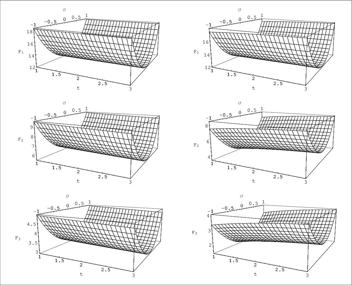
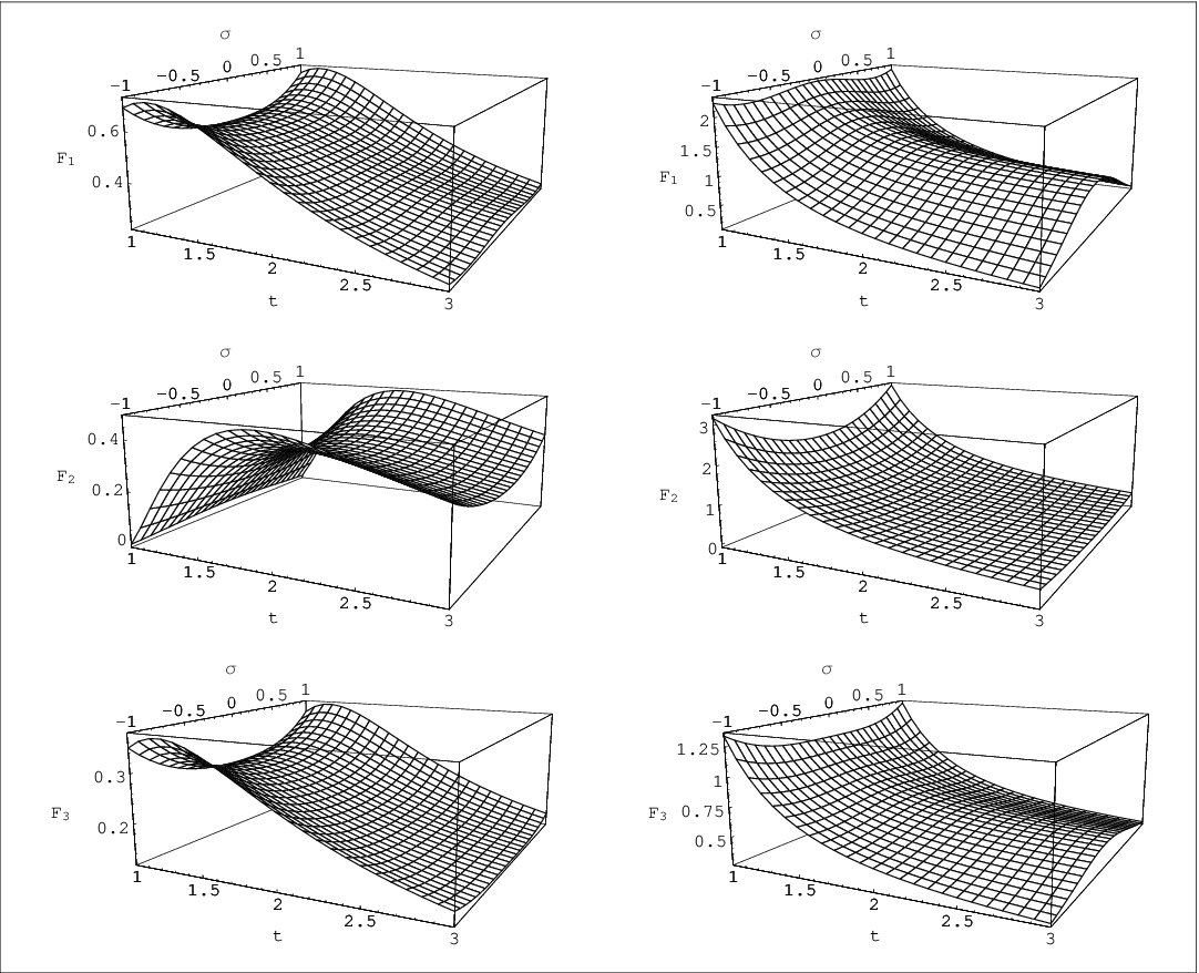
We find that for the above two models, all the inequalities are satisfied at least with the specific choices of parameters we have made. It has been checked that these inequalities can be satisfied in the presence of a decaying warp factor. However, for a growing warp factor (i.e. for a negative $b$ ) the inequalities are violated at least in some spacetime region.

IV Exact analytic solutions in the bulk

In this section, we discuss possible exact solutions in the bulk. We first assume an exponential warp factor and discuss some specific consequences for a given equation of state. In subsequent sub–sections, we look at exact solutions with different types of scalar fields – an ordinary massless scalar, the Brans-Dicke scalar and finally a dilatonic scalar.

IV.1 Models with an exponential (Randall–Sundrum type) warp factor

In the Randall-Sundrum scenario, the warp factor is of the form $f(\sigma)=-b|\sigma|$ . Using the functional form $f(\sigma)=-b\sigma$ (or $b\sigma$ ) and restricting ourselves to the $\sigma\geq 0$ (or $\sigma\leq 0$ ) region of the extra dimension, we now investigate some special cases by looking at the Einstein tensors and the resulting required matter stress-energy. To make things more quantitative, let us first write down the Einstein tensors with the above-mentioned warp factor.

$\displaystyle G_{00}$	$\displaystyle=$	$\displaystyle e^{2b\sigma}(3x^{2}+3xy)-\frac{6b^{2}}{\eta^{2}},$
$\displaystyle G_{\alpha\alpha}$	$\displaystyle=$	$\displaystyle-e^{2b\sigma}(2\dot{x}+3x^{2}+2xy+\dot{y}+y^{2})+\frac{6b^{2}}{\eta^{2}},$
$\displaystyle G_{44}$	$\displaystyle=$	$\displaystyle-e^{2b\sigma}(3\dot{x}+6x^{2})+\frac{6b^{2}}{\eta^{2}}$
$\displaystyle\mbox{and}\hskip 28.45274ptG_{04}$	$\displaystyle=$	$\displaystyle 3yb\frac{e^{b\sigma}}{\eta}$	(28)

(a) Let us first look at the situation where we have

G_{00}=-G_{\alpha\alpha}=-G_{44}.

(29)

Since the above relation holds for the factors associated with the $\frac{1}{\eta^{2}}$ terms in the Einstein tensors, conditions on $x$ , $y$ and its derivatives emerge when we impose identical conditions for the factors associated with the $e^{2b\sigma}$ terms. These conditions, after some elementary algebra lead to:

	$\displaystyle\dot{x}$	$\displaystyle=$	$\displaystyle-x^{2}+xy,$
	$\displaystyle\dot{y}$	$\displaystyle=$	$\displaystyle 2x^{2}-xy-y^{2}.$		(30)

Eq. 30 is an autonomous dynamical system of nonlinear first order differential equations. The general feature of all the solutions can be determined through a solution space analysis [14] of the above system. In this case, the line $x=y$ is a critical curve, i.e. every point on this line (except the origin) is a non-isolated fixed point. The eigenvalues of the Jacobian matrix (of the linearised system) at any such fixed point ( $x*,y*$ ) are ( $0,-4x*$ ), which suggests, for $x*>0$ fixed points are neutrally stable whereas for $x*<0$ they are neutrally unstable. It is difficult to make any conclusive comments, analytically, on the behaviour of phase space trajectories near those points, because such borderline cases are very sensitive to nonlinear terms in the equations. But the phase portrait (Fig.4) indeed confirms our conclusions about the nature of the fixed points. Note that, the ( $0,0$ ) point in the phase space is irrelevant as the Jacobian itself becomes singular and therefore it does not fall in any category of fixed points. From a physical point of view, the origin represents a static universe. We will see that no trajectory reaches that state in finite time. This provides a justification for the origin not representing a viable solution. Now, we turn our attention to the physically most preferable region of the solution space. This is the below–right quadrant, where $x$ is positive and $y$ is negative. There is one such curve, $x=-y$ , which is distinct from every other. It approaches the origin ( $0,0$ ), i.e. towards a static universe, as $t\rightarrow\infty$ . Any $(x,y)$ combination that is located above that line flows toward the line $x=y$ , resulting in the same scale factor for both kind of spatial dimensions, at $t=\infty$ . On the other hand, flows located below the curve $x=-y$ , tend toward a static brane ( $x=0$ ) with an extra dimension whose size shrinks, with ever increasing rate ( $y\rightarrow-\infty$ ), towards zero as $t\rightarrow\infty$ .

Following the phase portrait, we assume $y=nx$ , which implies, for consistency, $n^{2}=1$ or $n=\pm 1$ . The n=1 case is trivial because it leads to constant $a(t)$ and hence, constant $\eta(t)$ . With $n=-1$ we obtain, $a(t)\sim t^{\frac{1}{2}}$ and $\eta(t)\sim t^{-\frac{1}{2}}$ . This specific solution represents a radiative brane while the extra dimesion is indeed decaying (in accordance with our preference). For these forms of the $a(t)$ and $\eta(t)$ the stress energy is remarkably simple because, the coefficients of $e^{2b\sigma}$ in the Einstein tensors are all zero. Therefore, we just have:

T_{00}=-\frac{6b^{2}}{t}=-T_{\alpha\alpha}=T_{44},T_{04}=\frac{3b}{t}.

(31)

(b) We now move on to another case where we choose $a(t)=e^{\beta t}$ and $\eta(t)=e^{-\gamma t}$ with $\beta,\gamma>0$ while $f(\sigma)$ remains the same (i.e. $f(\sigma)\propto\sigma$ ). The Einstein tensors now take the form

$\displaystyle G_{00}$	$\displaystyle=$	$\displaystyle e^{2b\sigma}(3\beta^{2}-3\beta\gamma)-\frac{6b^{2}}{e^{-2\gamma t}},$
$\displaystyle G_{\alpha\alpha}$	$\displaystyle=$	$\displaystyle-e^{2b\sigma}(3\beta^{2}-2\beta\gamma+\gamma^{2})+\frac{6b^{2}}{e^{-2\gamma t}},$
$\displaystyle G_{44}$	$\displaystyle=$	$\displaystyle-e^{2b\sigma}(6\beta^{2})+\frac{6b^{2}}{e^{-2\gamma t}},$
$\displaystyle G_{04}$	$\displaystyle=$	$\displaystyle-3\gamma b\frac{e^{b\sigma}}{e^{-\gamma t}}.$	(32)

Notice that if $\beta=-\gamma$ , we end up with the same relations between the Einstein tensors as in (a) above, though this involves growing factors for both the cosmological scale and the extra dimension scale. In addition, we also note that with $\gamma=0$ one obtains a de-Sitter (or anti de-Sitter) brane with a constant scale for the extra dimension.

We now move on towards obtaining solutions in the true sense by assuming specific forms of the bulk energy momentum tensor.

IV.2 Bulk ordinary scalar

The simplest choice for a bulk energy momentum tensor is that of an ordinary, massless scalar field, for which we have:

T_{IJ}^{scalar}=\partial_{I}\phi\partial_{J}\phi-\frac{1}{2}g_{IJ}\partial_{K}\phi\partial^{K}\phi

(33)

with components, such as

	$\displaystyle T_{00}=\frac{e^{-2f}}{2}\dot{\phi}^{2}+\frac{\phi^{\prime 2}}{2\eta^{2}}=T_{44},\hskip 56.9055pt$
	$\displaystyle T_{\alpha\alpha}=\frac{e^{-2f}}{2}\dot{\phi}^{2}-\frac{\phi^{\prime 2}}{2\eta^{2}}\hskip 14.22636pt\mbox{and}\hskip 14.22636ptT_{04}=\dot{\phi}\phi^{\prime}\frac{e^{-f}}{\eta}.$		(34)

We now need to equate the above with the Einstein tensors and obtain solutions. To keep things simple, let us assume

\phi(t,\sigma)\equiv\phi_{1}(t)+\phi_{2}(\sigma).

(35)

From the equation for the $04$ component, we note that $\dot{\phi}_{1}=my$ and $\phi_{2}^{\prime}=\frac{3}{m}f^{\prime}$ . So, the form of $\phi(t,\sigma)$ will be

\phi(t,\sigma)=m\log[\eta(t)]+\frac{3}{m}f(\sigma)+const.

(36)

Using the relations between the coefficients of $\frac{1}{\eta^{2}}$ on both sides gives:

f(\sigma)=\frac{1}{4}\log(\sigma-\sigma_{0})+constant\hskip 14.45377pt;\hskip 14.45377pt{f^{\prime}}^{2}=12{\phi_{2}^{{}^{\prime}}}^{2}.

(37)

In the same way, using the relations between the coefficients of $e^{-2f}$ one gets:

	$\displaystyle\dot{x}$	$\displaystyle=$	$\displaystyle-3x^{2}-xy,$
	$\displaystyle\dot{y}$	$\displaystyle=$	$\displaystyle-y^{2}-3xy.$		(38)

We now further assume $y=nx$ which is consistent, for all n, with the above two equations for $\dot{x}$ and $\dot{y}$ . Therefore, solving the above two equations one finds

a(t)\sim(t-t_{1})^{\frac{1}{n+3}}\hskip 14.45377pt;\hskip 14.45377pt\eta(t)\sim(t-t_{2})^{\frac{n}{n+3}},

(39)

where $t_{1}$ and $t_{2}$ are integration constants. However, overall consistency requires that $m^{2}=\frac{3}{4}$ and $n=4\pm 2\sqrt{6}$ . For $n=4+2\sqrt{6}$ , both $a(t)$ and $\eta(t)$ are growing functions of time, which is a feature not desirable. On the other hand, for $n=4-2\sqrt{6}$ , we have the proper behaviour for $a(t)$ and $\eta(t)$ . The values of the exponents for $a(t)$ and $\eta(t)$ are quoted in Table 1. It is worth mentioning here that solutions of Eq. 38 are constrained by a consistency requirement of type $x\propto y$ , with a specific proportionality constant, which leaves us with solutions very few in number with respect to what we obtained in the case discussed earlier. Thus, a solution space analysis of Eq. 38 becomes irrelevant in this case. In fact, similar conclusions apply to the other two cases analysed below.

The case of the phantom scalar (with a negative kinetic energy) has also been investigated. Using the same methods, we find that solutions do not exist, primarily because, we end up having ${\phi^{\prime}}^{2}=-12\beta^{2}f^{\prime 2}$ , which is impossible, unless both sides are identically zero.

IV.3 Bulk Brans–Dicke scalar

Brans–Dicke theory [16] is well–known as an alternative theory of gravity where a scalar field $\phi$ is assumed to be responsible for generating the gravitational constant $G$ . Though experimentally almost ruled out, it serves as a useful model and, as mentioned later (see next section on dilaton gravity), it has also reappeared in various contexts in recent times. There have also been a few attempts [17, 18] towards constructing warped braneworld models in five-dimensional Brans-Dicke theory.

The action for Brans-Dicke gravity (in five dimensions and without a potential) where the Brans–Dicke scalar and the metric are the basic fields, is given as,

S=\frac{1}{16\pi}\int d^{5}x\sqrt{-g}\left[\phi R-\frac{\omega}{\phi}\phi_{,K}\phi_{,}^{K}+{\cal L}_{matter}\right]

(40)

In the above, we have assumed additional matter other than the scalar field itself (which, in a sense is not really matter, as such). The resulting Einstein’s equations and the scalar field equation are given as,

G_{IJ}=\frac{8\pi}{\phi}T_{IJ}+\frac{\omega}{\phi^{2}}\left[\phi_{,I}\phi_{,J}-\frac{1}{2}g_{IJ}\phi_{,K}\phi_{,}^{K}\right]+\frac{\phi_{;I;J}-g_{IJ}\Box\phi}{\phi},

(41)

2\omega\frac{\Box\phi}{\phi}+R-\omega\frac{(\nabla\phi)^{2}}{\phi^{2}}=0.

(42)

Contracting Eq. 41 and substituting in Eq. 42, we get

\Box\phi=\frac{8\pi}{4+3\omega}T

(43)

where $T$ denotes the trace of the matter energy momentum tensor.

IV.3.1 Solutions with perfect fluid bulk matter

Let us choose the bulk matter energy momentum tensor to be that of a perfect fluid, $T_{IJ}=diag(\rho,p_{\alpha},p_{\alpha},p_{\alpha},p_{\sigma})$ , with a vanishing trace

T=-\rho+3p_{\alpha}+p_{\sigma}=0.

(44)

Thus the scalar field equation essentially becomes

\Box\phi=-e^{-2f}\left[\ddot{\phi}+\left(3\frac{\dot{a}}{a}+\frac{\dot{\eta}}{\eta}\right)\dot{\phi}\right]+\frac{1}{\eta^{2}}\left[\phi^{\prime\prime}+4f^{\prime}\phi^{\prime}\right]=0

(45)

Then assuming $\phi(t,\sigma)=\phi_{1}(t)\phi_{2}(\sigma)$ , the Einstein’s equations yield,

\displaystyle G_{00}=e^{-2f}\left(\frac{\ddot{\phi}_{1}}{\phi_{1}}+\frac{\omega}{2}\frac{\dot{\phi}_{1}^{2}}{\phi_{1}^{2}}\right)-\frac{1}{\eta^{2}}\left(-\frac{\omega}{2}\frac{\phi_{2}^{\prime 2}}{\phi_{2}^{2}}+f^{\prime}\frac{\phi_{2}^{\prime}}{\phi_{2}}\right)+8\pi\frac{\rho}{\phi},

\displaystyle G_{\alpha\alpha}=e^{-2f}\left(\frac{\omega}{2}\frac{\dot{\phi}_{1}^{2}}{\phi_{1}^{2}}-x\frac{\dot{\phi}_{1}}{\phi_{1}}\right)+\frac{1}{\eta^{2}}\left(-\frac{\omega}{2}\frac{\phi_{2}^{\prime 2}}{\phi_{2}^{2}}+f^{\prime}\frac{\phi_{2}^{\prime}}{\phi_{2}}\right)+8\pi\frac{p_{\alpha}}{\phi},

\displaystyle G_{44}=e^{-2f}\left(\frac{\omega}{2}\frac{\dot{\phi}_{1}^{2}}{\phi_{1}^{2}}-y\frac{\dot{\phi}_{1}}{\phi_{1}}\right)+\frac{1}{\eta^{2}}\left(\frac{\phi_{2}^{\prime\prime}}{\phi_{2}}+\frac{\omega}{2}\frac{\phi_{2}^{\prime 2}}{\phi_{2}^{2}}\right)+8\pi\frac{p_{\sigma}}{\phi},

\mbox{and}\hskip 28.45274ptG_{04}=\frac{e^{-f}}{\eta}\left[(\omega+1)\frac{\dot{\phi}_{1}\phi_{2}^{\prime}}{\phi_{1}\phi_{2}}-f^{\prime}\frac{\dot{\phi}_{1}}{\phi_{1}}-y\frac{\phi_{2}^{\prime}}{\phi_{2}}\right].

(46)

Using the expressions for the Einstein tensor components, as given in Eq. 10, the off-diagonal term in the Einstein equations leads to the following possibility,

\frac{\dot{\phi}_{1}}{\phi_{1}}=my\hskip 14.22636pt\mbox{and}\hskip 14.22636pt\frac{\phi_{2}^{\prime}}{\phi_{2}}=nf^{\prime}\hskip 14.22636pt\mbox{where}\hskip 14.22636ptm=\frac{3+n}{\frac{4n}{3}-1}.

(47)

Thus, we have,

\phi(t,\sigma)\sim\eta^{m}(t)e^{nf(\sigma)}.

(48)

Now, dividing Eq. 45 by $\phi$ , separately equating the coefficients of $e^{-2f}$ and $\frac{1}{\eta^{2}}$ to zero and using 47 we get,

	$\displaystyle\dot{y}+3xy+(m+1)y^{2}$	$\displaystyle=$	$\displaystyle 0$		(49)
	$\displaystyle\mbox{and}\hskip 28.45274ptf^{\prime\prime}+(n+4)f^{\prime 2}$	$\displaystyle=$	$\displaystyle 0$		(50)

Similarly, using diagonal components of Einstein equations and Eq. 49, tracelessness of $T_{IJ}$ (Eq. 44) leads to,

	$\displaystyle\dot{x}+2x^{2}-Ay^{2}=0,\hskip 28.45274pt\mbox{where}\hskip 28.45274ptA=\frac{m}{3}\left(1-\frac{m\omega}{2}\right)$		(51)
	$\displaystyle\mbox{and}\hskip 28.45274pt(12-n)f^{\prime\prime}+\left(\frac{3\omega}{2}n^{2}-n^{2}-4n+30\right)f^{\prime 2}=0$		(52)

Consistency requirement between Eq. 50 and Eq. 52 gives rise to the following condition,

n_{\pm}=\frac{4\pm 2\sqrt{4+3\omega}}{\omega}\hskip 28.45274pt\mbox{which also implies}\hskip 28.45274ptm_{\pm}=\frac{3}{\pm\frac{10}{\sqrt{4+3\omega}}-1}.

(53)

Then Eq. 50 results in

f(\sigma)=const.+\frac{1}{4+n}\log(\sigma-\sigma_{0}).

(54)

It may be noted that, the factor $\frac{1}{4+n}$ is always positive for $n=n_{-}$ , but it can be negative as well for $n=n_{+}$ , which implies both growing and decaying warp factor solutions are possible.

It is evident that Eq. 49 and Eq. 51 constitute a dynamical system of their own for every possible value of $\omega$ . At the critical point (0,0), the Jacobian of the linearised system vanishes. Therefore, let us directly look at the phase portraits (Fig. 5) of this system for $m=m_{+}$ (left plot) and $m=m_{-}$ (right plot) at, for example, $\omega=1$ .

Cosmologically viable features are apparent in the x-positive (expanding brane) and y-negative (decaying extra dimension) quadrant of both the phase spaces. In the left-side plot, one class of trajectories flow towards the centre, as time increases. Another class of trajectories flow toward $y=-\infty$ (extra dimension decaying at an ever increasing rate) solution as $t\rightarrow\infty$ , while the $x$ -coordinate increases very less. Now, $x$ becoming almost constant, in turn implies an almost exponential growth of $a(t)$ or brane inflation. In this case, this can mean that the brane expands very rapidly and forever – a big rip.

On the other hand, in the right-side plot, one class of x-positive and y-negative solutions flow towards the centre , which represents a static universe and another class of trajectories flow toward $x=-\infty$ and $y=-\infty$ (whole of the space is singular at this point) while crossing the y-axis ( $x=0$ ) very slowly. This means the expansion of the brane first slows down to staticity and then starts contracting – a big crunch. Another crossover takes place from x-negative and y-positive quadrant to x-positive and y-positive quadrant, for certain initial conditions, and then these trajectories flow towards the centre. Some part of these trajectories become parallel to $y$ -axis, i.e. $x$ become constant, for a very short span of time, which can cause brane inflation, though the extra dimension is also of the growing type.

IV.3.2 The vacuum solution

Now, let us assume

y=hx,

(55)

i.e. we are considering the straight lines in the phase spaces at all values of $\omega$ . Then the consistency requirement between Eq. 49 and Eq. 51 leads to the following condition

Ah^{2}+(m+1)h^{2}+1=0\hskip 14.22636pt\Rightarrow\hskip 14.22636pth_{\pm}=\frac{-(m+1)\pm\sqrt{(m+1)^{2}-4A}}{2A}.

(56)

When the abovementioned constraint is satisfied, our job reduces to solving only one independent equation

\dot{x}=(Ah^{2}-2)x.

(57)

Integrating further, we eventualliy get

a(t)\sim t^{\frac{1}{2-Ah^{2}}}\hskip 28.45274pt\mbox{and}\hskip 28.45274pt\eta(t)\sim t^{\frac{h}{2-Ah^{2}}}.

(58)

The most interesting feature of this specific set of solutions is that, these are actually vacuum solutions, i.e. one can easily check that all the matter energy momentum tensor components identically vanish when Eq. 56 is satisfied. The following figure gives a view of the exponents in $a(t)$ ( $\nu_{1}=\frac{1}{2-Ah^{2}}$ ) and $\eta(t)$ ( $\nu_{2}=\frac{h}{2-Ah^{2}}$ ) as functions of $\omega$ .

It can be clearly seen that all possible combinations of $\nu_{1}$ and $\nu_{2}$ (+ve+ve, +ve-ve, -ve+ve and -ve-ve) are there at different values of $\omega$ . In fact, the variations seem to suggest that an expanding brane mostly suits a decaying extra dimension.

IV.3.3 The radiative solution

One specific case, where an analytic solution is possible, is when $A=0$ , i.e. for $\omega=1.586$ , we have

	$\displaystyle\dot{x}$	$\displaystyle=$	$\displaystyle-2x^{2}$		(59)
	$\displaystyle\dot{y}$	$\displaystyle=$	$\displaystyle-3xy-2.26y^{2}.$		(60)

Which implies,

	$\displaystyle x$	$\displaystyle=$	$\displaystyle\frac{1}{2t-c_{1}}$		(61)
	$\displaystyle\mbox{and}\hskip 28.45274pty$	$\displaystyle=$	$\displaystyle\frac{1}{(2t-c_{1})(c_{2}\sqrt{2t-c_{1}}-2.26)},$		(62)

where $c_{1}$ and $c_{2}$ are integration constants, whose different values will span the whole solution space of $x$ and $y$ for the abovementioned value of $\omega$ . It may also be noted that, with $c_{2}=0$ , we have the vacuum solution for $\omega=1.586$ (in which case the extra dimension is essentially decaying again). Further, integrating Eq. 61 and Eq. 62 we get,

	$\displaystyle a(t)$	$\displaystyle\sim$	$\displaystyle(2t-c_{1})^{\frac{1}{2}}$		(63)
	$\displaystyle\mbox{and}\hskip 28.45274pt\eta(t)$	$\displaystyle\sim$	$\displaystyle\frac{(2.26-c_{2}\sqrt{2t-c_{1}})^{0.44}}{(2t-c_{1})^{0.22}}.$		(64)

The above solution, in fact, represents a radiative brane while the nature of the extra dimension depends on $c_{1}$ and $c_{2}$ . Fig. 7 shows how the nonzero components of matter energy momentum tensor, $\rho$ and $p_{\alpha}$ ( $p_{\sigma}$ vanishes in this case), behave as function $t$ and $\sigma$ with $c_{1}=0$ and $c_{2}=1$ .

IV.3.4 Solutions in Brans-Dicke frame using Einstein frame scalar field solutions

It is well known that the action of Brans–Dicke theory, as stated in the previous section, can be converted into that of canonical Einstein gravity coupled to a massless scalar field. We recall below how this is done. First, let us rewrite the action for Brans Dicke theory replacing $\phi$ by $e^{-2{\tilde{\phi}}}$ and $g_{IJ}$ by ${\tilde{g}}_{IJ}$ . Subsequently, defining a conformally related metric

{{\tilde{g}}}_{IJ}=\Omega^{2}(\sigma,t)g_{IJ}

(65)

and choosing $\Omega=e^{\frac{2}{3}{\tilde{\phi}}}$ we find that the Brans–Dicke action (with no additional matter fields) goes over to:

S=\int d^{5}x\sqrt{-g}\left[R-\frac{4}{3}\left(4+3\omega\right)g^{IJ}\nabla_{I}{\tilde{\phi}}\nabla_{J}{\tilde{\phi}}\right].

(66)

Further, defining:

\Phi=\frac{2}{3}\sqrt{4+3\omega}{\tilde{\phi}}

(67)

we can convert the action above into that of Einstein gravity coupled to an ordinary scalar field.

This equivalence can now be used to construct new solutions in Brans–Dicke theory by making use of the solutions with an ordinary scalar field discussed earlier in Section IV B. The main point here is that the solutions with an ordinary scalar are also solutions of Brans–Dicke theory in the Einstein canonical frame. How do these solutions look like in the Brans–Dicke frame? We look at this aspect now.

Following the earlier ordinary scalar field analysis we choose:

\Phi=m\ln\eta+\frac{3}{m}f

(68)

with $a(t)\sim(t-t_{0})^{\frac{1}{n+3}}$ , $\eta(t)\sim(t-t_{0})^{\frac{n}{n+3}}$ and $f(\sigma)=\frac{1}{4}\ln(\sigma-\sigma_{0})$ . We also had $m^{2}=\frac{3}{4}$ and $n=4\pm 2\sqrt{6}$ .

The metric in the Brans–Dicke frame is related to that in the Einstein frame by an overall conformal factor $\Omega^{2}=e^{\frac{4}{3}{\tilde{\phi}}}$ . Using the relation between $\tilde{\phi}$ and $\Phi$ we find that the conformally related line element becomes:

ds^{2}=e^{2f_{1}(\sigma_{1})}\left[-d\tau^{2}+a_{1}^{2}(\tau){|d\vec{x}|}^{2}\right]+\eta_{1}^{2}(\tau)d\sigma_{1}^{2}

(69)

where:

	$\displaystyle\tau-\tau_{0}=\frac{(t-t_{0})^{p+1}}{p+1}\hskip 7.22743pt;\hskip 7.22743pt\sigma_{1}-\bar{\sigma}_{1}=\frac{(\sigma-\sigma_{0})^{q+1}}{q+1}$		(70)
	$\displaystyle p=\frac{mn}{(n+3)\sqrt{3(4+3\omega)}}\hskip 7.22743pt;\hskip 7.22743ptq=\frac{3}{4m\sqrt{3(4+3\omega)}}$		(71)

and

$\displaystyle f_{1}(\sigma_{1})$	$\displaystyle=$	$\displaystyle const.+\frac{4q+1}{4q+4}\log(\sigma_{1}-\bar{\sigma}_{1}),$	(72)
$\displaystyle a_{1}(\tau)$	$\displaystyle\sim$	$\displaystyle(\tau-\tau_{0})^{\frac{p(n+3)+1}{(p+1)(n+3)}},$	(73)
$\displaystyle\eta_{1}(\tau)$	$\displaystyle\sim$	$\displaystyle(\tau-\tau_{0})^{\frac{p(n+3)+n}{(p+1)(n+3)}}.$	(74)

We now illustrate the nature of the coefficient in $f_{1}$ and the exponents in $a_{1}$ and $\eta_{1}$ appearing in the above solutions as functions of $\omega$ for the four possible combinations of (m,n) through Fig. 8.

It is interesting to note that for set(i) and set(iii) growing $a_{1}(\tau)$ - decaying $\eta_{1}(\tau)$ combination does not exist whereas for set (ii) and set(iv) both decaying and growing warp factor solutions exist with desired evolutions for $a_{1}(\tau)$ and $\eta_{1}(\tau)$ .

IV.4 Bulk dilaton scalar

Low energy effective string theory gives rise to Einstein-like equations through the conditions that the $\beta$ -functions of the string $\sigma$ -model are equal to zero [1]. The Einstein like equations have additional terms involving the dilaton (a scalar), third rank antisymmetric tensor and other fields (Maxwell and moduli fields) which arise out of the method of compactification. Dilaton gravity involves only the dilaton and the metric field. It is different from ordinary scalar field theory and is equivalent to Brans-Dicke theory under a special choice of the $\omega$ parameter (being set equal to -1). The action for dilaton gravity [15] is given as:

S=\int{d^{5}x\sqrt{-g}e^{-2\phi}(R+4\partial_{K}\phi\partial^{K}\phi)}.

(75)

This gives the following field equations,

	$\displaystyle G_{IJ}=-2\nabla_{I}\nabla_{J}\phi+g_{IJ}\nabla^{2}\phi,$		(76)
	$\displaystyle g^{IJ}\nabla_{I}\nabla_{J}\phi=2g^{IJ}\nabla_{I}\phi\nabla_{J}\phi.$		(77)

IV.4.1 A solution in the string frame

The terms in the R. H. S. of the above equation can be clubbed together to yield an effective energy momentum tensor. The effective matter stress energy is therefore given as:

$\displaystyle\mbox{ie.}\hskip 28.45274ptT_{00}$	$\displaystyle=$	$\displaystyle e^{-2f}(-\ddot{\phi}+(3x+y)\dot{\phi})-\frac{1}{\eta^{2}}(\phi^{\prime\prime}+2f^{\prime}\phi^{\prime}),$
$\displaystyle T_{\alpha\alpha}$	$\displaystyle=$	$\displaystyle-e^{-2f}(\ddot{\phi}+(x+y)\dot{\phi})+\frac{1}{\eta^{2}}(\phi^{\prime\prime}+2f^{\prime}\phi^{\prime}),$
$\displaystyle T_{44}$	$\displaystyle=$	$\displaystyle-e^{-2f}(\ddot{\phi}+(3x-y)\dot{\phi})+\frac{1}{\eta^{2}}(-\phi^{\prime\prime}+4f^{\prime}\phi^{\prime})$
$\displaystyle\mbox{and}\hskip 28.45274ptT_{04}$	$\displaystyle=$	$\displaystyle\frac{e^{-f}}{\eta}(-2\partial_{t}\partial_{\sigma}\phi+2f^{\prime}\dot{\phi}+2y\phi^{\prime}).$	(78)

Let us assume, as before,

\phi(t,\sigma)\equiv\phi_{1}(t)+\phi_{2}(\sigma).

(79)

Then the off–diagonal term in the Einstein equations gives us the following constraints,

\dot{\phi}_{1}=my\hskip 14.22636pt\mbox{and}\hskip 14.22636pt\phi_{2}^{\prime}=nf^{\prime}\hskip 14.22636pt\mbox{where}\hskip 14.22636ptm=\frac{3-2n}{2}.

(80)

So, essentially we have,

\phi(t,\sigma)=m\log[\eta(t)]+nf(\sigma)+const.

(81)

Now, equating the coefficients of $\frac{1}{\eta^{2}}$ in the both sides of the Einstein’s equations we get,

	$\displaystyle f^{\prime\prime}(\sigma)+\frac{6-4n}{n}f^{\prime 2}(\sigma)=0$		(82)
	$\displaystyle\hskip 14.22636pt\mbox{and}\hskip 14.22636pt(m,n)\equiv\left(\frac{1}{2},1\right)\hskip 8.5359pt\mbox{or}\hskip 8.5359pt\left(-\frac{3}{2},3\right).$		(83)

On the other hand, equating the coefficient of $\frac{1}{\eta^{2}}$ in the scalar field equation gives:

f^{\prime\prime}(\sigma)+\frac{4-2n}{n}f^{\prime 2}(\sigma)=0

(84)

Thus the only allowed value for (m,n) is $m=\frac{1}{2}$ and $n=1$ which gives:

f(\sigma)=const.+\frac{1}{2}\log(\sigma-\sigma_{0}),\hskip 28.45274pt\mbox{a growing warp factor,}

(85)

Finally, equating the the coefficients of $e^{-2f}$ in the Einstein equations (with $m=\frac{1}{2}$ ), we get,

$\displaystyle 3x^{2}+\frac{3}{2}xy+\frac{1}{2}\dot{y}-\frac{1}{2}y^{2}$	$\displaystyle=$	$\displaystyle 0,$
$\displaystyle 2\dot{x}+3x^{2}+\frac{3}{2}xy+\frac{1}{2}\dot{y}+\frac{1}{2}y^{2}$	$\displaystyle=$	$\displaystyle 0$
$\displaystyle\mbox{and}\hskip 28.45274pt3\dot{x}+6x^{2}-\frac{1}{2}\dot{y}-\frac{3}{2}xy+\frac{1}{2}y^{2}$	$\displaystyle=$	$\displaystyle 0.$	(86)

The three coupled equations above give rise to the following algebraic constraint,

3x^{2}-\frac{1}{2}y^{2}=0.

(87)

which yields

y=\pm\sqrt{6}x,\hskip 14.22636pt\frac{\ddot{a}}{a}+2\frac{\dot{a}^{2}}{a^{2}}=0\hskip 14.22636pt\mbox{and}\hskip 14.22636pt\frac{\ddot{\eta}}{\eta}+\left(\pm\sqrt{\frac{3}{2}}-1\right)\frac{\dot{\eta}^{2}}{\eta^{2}}=0,

(88)

with solutions as,

a(t)\sim(t-t_{0})^{\frac{1}{3}}\hskip 14.22636pt\mbox{and}\hskip 14.22636pt\eta(t)\sim(t-t_{0})^{\pm\sqrt{\frac{2}{3}}}.

(89)

Note that the coefficient of $e^{-2f}$ in the scalar field equation gives $\dot{y}+3xy=0$ , which is automatically satisfied by the abovementioned solution. We discard the positive exponent solution for $\eta$ , on physical grounds discussed before.

IV.4.2 Solutions in string frame using Einstein-scalar solutions in Einstein frame

It has been noted earlier that for $\omega=-1$ , Brans–Dicke theory gives rise to dilaton gravity. Using the solutions for Einstein gravity coupled to an ordinary scalar we now construct string (Brans–Dicke) frame solutions in dilaton gravity, following the discussion presented in IV B.

Substituting $\omega=-1$ in Eqns. 72-74 we get the following forms for $a_{1}(\tau)$ , $\eta_{1}(\tau)$ and $f_{1}(\sigma_{1})$ .

	$\displaystyle f_{1}(\sigma_{1})=const.+\frac{4q+1}{4q+4}\log(\sigma_{1}-\bar{\sigma}_{1}),$		(90)
	$\displaystyle a_{1}(\tau)=\left[(p+1)(\tau-\tau_{0}\right]^{\frac{p(n+3)+1}{(p+1)(n+3)}},$		(91)
	$\displaystyle\eta_{1}(\tau)=\left[(p+1)(\tau-\tau_{0})\right]^{\frac{p(n+3)+n}{(p+1)(n+3)}}.$		(92)

with $p=\frac{mn}{\sqrt{3}(n+3)}$ , $q=\frac{\sqrt{3}}{4m}$ and $m=\pm\frac{\sqrt{3}}{2}$ , $n=4\pm 2\sqrt{6}$ .

The four sets for $a_{1}$ , $\eta_{1}$ and $f_{1}$ (correspomding to four different combination of ( $m,n$ )) yield two acceptable solutions – one with a decaying warp factor and another with a growing warp factor (this is in fact the same solution as given by Eq. 89). Fig.9 shows the nature of these solutions in presence of bulk dilaton field.

The explicit solutions (those which are physically meaningful) are displayed in Table I.

V Status of energy conditions for the above solutions

We now focus our attention on analysing the energy conditions some of the above solutions.

Bulk Field	$f(\sigma)=const.+$	$a(t)\sim$	$\eta(t)\sim$	$F_{1}\geq 0$	$F_{2}\geq 0$	$F_{3}\geq 0$
Ordinary Scalar	$0.25\log(\sigma-\sigma_{0})$	$(t-t_{0})^{0.48}$	$(t-t_{0})^{-0.43}$	$\surd$	$\times$	$\surd$
Brans-Dicke (for $\omega=1$ )	$0.37\log(\sigma-\sigma_{0})$	$(t-t_{0})^{0.43}$	$(t-t_{0})^{-0.55}$	$\surd$	$\times$	$\surd$
Brans-Dicke (for $\omega=1$ )	$0.075\log(\sigma-\sigma_{0})$	$(t-t_{0})^{0.515}$	$(t-t_{0})^{-0.32}$	$\surd$	$\surd$	$\surd$
Dilaton Scalar ( $\omega=-1$ )	$0.5\log(\sigma-\sigma_{0})$	$(t-t_{0})^{0.33}$	$(t-t_{0})^{-0.82}$	$\times$	$\times$	$\surd$
Dilaton Scalar ( $\omega=-1$ )	$-0.5\log(\sigma-\sigma_{0})$	$(t-t_{0})^{0.57}$	$(t-t_{0})^{-0.18}$	$\surd$	$\surd$	$\surd$

Table 1: The above table shows few of the typical solutions, found in Section IV, mentioning their desirability as viable models and the status of the energy condition inequalities (Eqs. 23, 24, 25).

In Table 1, we have listed the ‘good’ solutions (only those which have a combination of growing cosmological scale and a decaying extra dimensional scale) found in the previous sections. For the Brans-Dicke case ,we have two solutions for $\omega=1$ . The solutions with a dilaton field are essentially derived from general solutions for the Brans-Dicke case by just equating $\omega=-1$ . There are solutions with both decaying and growing warp factors. Notably, all solutions have singularities at a finite value of $t$ or $\sigma$ . To investigate the status of WEC for these solutions, we have plotted the inequality functions. It is found that the 3rd and 5th set of solutions satisfy all the inequalities (Fig.10). Here, the statement inequality is satisfied means that it is satisfied in an entire semi-infinite spacetime region from {( $t=t_{c},\sigma=\sigma_{c}$ ) to ( $t=\infty,\sigma=\infty)$ }, where $t_{c}$ and $\sigma_{c}$ are suitably chosen lower bounds (these bounds essentially comes from the constraint inequality relation 22) on the allowed domain for $t$ and $\sigma$ (energy condition satisfying solutions have to be defined in these domains only). The statement not satisfied means that no semi-infinite spacetime region can be found where energy conditions are satisfied.

VI Placing the Brane and Singularity Resolution

Till now we have essentially found bulk solutions. To have a proper brane-bulk system, we need to place a four dimensional hypersurface in the bulk. One can do this by replacing the argument of the logarithm (appearing in every solution of $f(\sigma)$ ), i.e. $\sigma$ , by $|\sigma|$ . The contribution of this modulus function will appear as a Dirac delta function peaked at some $\sigma_{b}$ (which is the location of the brane), in the left hand side of Einstein equations. To justify this, the energy momentum tensor on the right hand side of Einstein equations must carry a delta-peaked term too. This can be done by adding an extra term multiplied with a delta function in the bulk Lagrangian, which also peaks at the location where we intend to place the thin brane.

VI.1 Junction conditions

Let us take the contribution of the brane to the Einstein-Hilbert action to be,

S_{b}=-\int{d^{4}x\sqrt{-g_{4}}\ \lambda(\phi)}\equiv-\int{d^{5}x\sqrt{-g_{5}}\ \lambda(\phi)}\frac{\delta(\sigma-\sigma_{b})}{\sqrt{g_{44}}}.

(93)

Here $g_{5}$ denotes the determinant of the full five-dimensional bulk metric and $g_{4}$ is the determinant of the induced metric on the brane. Now, we can determine the jump in $f^{\prime}(\sigma)$ (or $\phi^{\prime}(\sigma)$ ) across the brane, from the junction conditions [19], in the model cases of the ordinary scalar field or the Brans-Dicke field coupled to gravity.

VI.1.1 Junction conditions with ordinary scalar field

Integrating the scalar field equation at the location of the brane, we get,

\big[\phi_{2}^{\prime}\big]=\frac{\eta}{2}\frac{d\lambda}{d\phi}\ \Bigg|_{\sigma=\sigma_{b}}

(94)

Then from Einstein equations we have,

\big[f^{\prime}\big]=-\frac{\eta}{6}\lambda\ \Bigg|_{\sigma=\sigma_{b}}

(95)

Now, using the constraint $\phi_{2}^{\prime}=\frac{3}{m}f^{\prime}$ , we obtain,

\lambda(\phi)=\lambda_{0}\ e^{-\frac{\phi}{m}},

(96)

where $\lambda_{0}$ is an integration constant. For the above expression of $\lambda(\phi)$ , junction conditions 94 and 95, in fact, become independent of $\eta(t)$ (similar feature is reported in [6]).

VI.1.2 Junction conditions with Brans-Dicke field

Similarly, in the Brans-Dicke case, the scalar field equation (Eq. 42) at the location of the brane (with the brane tension given by Eq. 93) gives us,

-4\big[f^{\prime}\big]+2\omega\frac{\big[\phi_{2}^{\prime}\big]}{\bar{\phi}}=\frac{\eta}{2}\frac{d\lambda}{d\phi}\ \Bigg|_{\sigma=\sigma_{b}}.

(97)

where $\bar{\phi}$ is, the mean value of the function $\phi(t,\sigma)$ at $\sigma=\sigma_{b}$ , defined as

\bar{\phi}=\frac{\phi(\sigma_{b}^{+})+\phi(\sigma_{b}^{-})}{2}.

(98)

Further, from the $00$ or $\alpha\alpha$ component of the Einstein equations, we get,

3\big[f^{\prime}\big]=-\frac{\eta}{2}\lambda\ \Bigg|_{\sigma=\sigma_{b}},

(99)

Using the relation $\frac{\phi^{\prime}}{\phi}=nf^{\prime}$ , leads us to

\lambda(\phi)=\lambda_{0}\ e^{-\frac{2n\omega-4}{3}\phi},

(100)

for which the junction condition becomes,

\big[f^{\prime}\big]=-\frac{\lambda_{0}}{6}\eta\ e^{-\frac{2n\omega-4}{3}\bar{\phi}}.

(101)

In this case, the junction conditions are time dependent.

The junction conditions for the dilaton case can be obtained by using $\omega=-1$ and a redefinition of the $\phi$ field in the above analysis for the Brans–Dicke scalar.

VI.2 Resolving bulk singularities

It may be noted that all our solutions (except those discussed under the section on an exponential RS type warp factor) have bulk singularities, apart from the usual big-bang cosmological singularity in time. The latter is inevitable and expected while the former needs better understanding.

The main question we need to address is – how do we manage to use a spacetime with a bulk singularity as a model for our bulk five dimensional geometry? There are ways to do this.

One possible resolution of the singularities is done by putting branes at the locations of the singularities. For example, let us take, in the case of solutions with a bulk dilaton field, the two different solutions valid in two different regions (except the points where singularities occur), i. e.

f(\sigma)=\left\{\begin{array}[]{ll}\frac{1}{2}\log|\sigma-\sigma_{1}|+c_{1},\hskip 28.45274pt\mbox{for}\hskip 28.45274pt\sigma\leq\sigma_{0}\\ -\frac{1}{2}\log|\sigma-\sigma_{2}|+c_{2},\hskip 28.45274pt\mbox{for}\hskip 28.45274pt\sigma\geq\sigma_{0}\end{array}\right.

(102)

where $\sigma_{0}$ is located somewhere between $\sigma_{1}$ and $\sigma_{2}$ . Then continuity at $\sigma_{0}$ implies,

\frac{1}{2}\log|\sigma_{0}-\sigma_{1}|+c_{1}=-\frac{1}{2}\log|\sigma_{0}-\sigma_{2}|+c_{2},

(103)

Now this is a good bulk solution except at points $\sigma_{1}$ and $\sigma_{2}$ . To resolve these singularities we can put two branes at $\sigma_{1}$ and $\sigma_{2}$ and another brane at $\sigma_{0}$ and make their total contribution to bulk vacuum energy vanish [20] (as we do not have any bulk cosmological constant). This will be equivalent to putting delta-function source terms in the bulk Lagrangian. In effect, those singularities in bulk solutions actually provide us with places for the 3–branes, one of which can be chosen to be the Standard Model brane we live in.

VII Conclusions

Finally, we list below, systematically, the conclusions obtained in this investigation.

•

We start out by writing down the energy condition inequalities using the Einstein tensor components (which have a nonzero $G_{04}$ ). These inequalities are first checked for typical choices for the various metric functions $a(t)$ , $\eta(t)$ and $f(\sigma)$ . We demonstrate that there exist viable models (following the criteria listed in the Introduction) which satisfy the energy conditions.
•

We also find exact solutions with matter sources of various kinds. To begin with, we look at possible matter sources that may arise if we assume an exponential (in $\sigma$ ) warp factor and some other typical constraints on matter stress energy. The solution space for $[a(t),\eta(t)]$ is analysed using a dynamical systems approach. Subsequently, we look at solutions with various types of scalar fields as sources – eg. bulk normal scalar, the Brans-Dicke scalar and the dilaton scalar. In our approach to obtaining solutions we exploit the known fact that with a conformally related metric and a redefined scalar one can convert BD theory into canonical Einstein Gravity coupled to a scalar. Analytic solutions are written down and the various possibilities that arise are outlined. In the case with a Brans-Dicke scalar and matter in the bulk, it is observed that, for traceless matter energy momentum exact and viable analytical solutions can be found with decaying or growing warp factors as well as decelerating/accelerating $a(t)$ . We note that in the case of the dilaton we can have decaying as well as growing warp factor solutions too. We are also able to find desirable solutions with growing $a(t)$ and decaying $\eta(t)$ in several of our examples.
•

We check the energy conditions, the nature of the functions $a(t)$ and $\eta(t)$ and figure out whether an obtained solution is desirable or not. The details are tabulated in one of the columns in the table commenting on the desirability of the solution. We do find several classes of desirable solutions, which satisfy our requirements and the energy conditions.
•

Finally, we outline how one can place a brane in the above bulk spacetimes by using the junction conditions . We also briefly discuss a way to resolve the bulk singularities using standard techniques.

With three different functions appearing in the line element, it is always very difficult to find exact solutions. That we have found some is indeed encouraging. We hope to use these solutions in actual brane cosmological scenarios and arrive at relevant conclusions by making use of existing observational data on supernova and CMB anisotropies. We would also like to extend our results to other types of stress energy expressions. A disturbing aspect of our solutions is that they are singular in the bulk, though we do provide ways of resolving them. It remains to be seen whether we can find newer solutions (a) which are not necessarily of a power law type, (b) which have, in appropriate limits, both deceleration and acceleration, (c) which have a decaying extra dimension stabilisable to a finite value and (d) where the bulk warp factor gives rise to a non-singular bulk metric, similar to RS. In essence, an appropriate combination of different bulk fields, with some dominating over the others in specific time intervals, will then be able to generate the expansion history (with proper decelerating and accelerating phase), of our universe on the brane.

Acknowledgements

SG thanks IIT Kharagpur for providing financial support and Centre for Theoretical Studies, IIT Kharagpur for its research facilities. We also thank P. S. Dutta for useful discussions.

References

[1] M. S. Green, J. H. Schwarz and E. Witten, Superstring Theory, Camebridge University press, Camebridge, U.K., 1987.
[2] L. Randall and R. Sundrum, Phys. Rev. lett. 83 (1999) 3370; L. Randall and R. Sundrum, Phys. Rev. lett. 83 (1999) 4690.
[3] Th. Kaluza, Sitzunober. Preuss. Akad. Wiss. Berlin, 966 (1921); O. Klein, Z. Phys. 37 (1926) 895.
[4] D. J. H. Chung and K. Freese, Phys. Rev. D 61 023511 (1999);
[5] Hongya Liu and B. Mashhoon, Ann. Phys. (Leipzig) 4, 565 (1995); G. W. Gibbons, R. Gueven and C. N. Pope, Phys. lett. B 595, 498, (2004). A. Wong, R-G Cai and N. O. Santos, Nucl. Phys. B 797, 395 (2008); S. Pal and S. Kar, Gen.Rel.Grav.41:1165-1179,2009 (and references therein); I. Neupane, [arXiv:0903.4190].
[6] K. Koyama and K. Takahashi, Phys. Rev. D68 103512 (2003).
[7] Je-An Gu, W-Y. P. Hwang, Phys. Rev. D 66 024003 (2002), K. Freese and M.Lewis, Phys. Letts. B 540, 1 (2002); J. M. Cline and J. Vinet, Phys. Rev. D 68 025015 (2003).
[8] K. C. Chan and M.-C. Chu, Phys. Rev. D 76 043525 (2007); Phys. Rev. D 77 063525 (2008).
[9] B. Li and M.-C. Chu, Phys. Rev. D 73 025004 (2006); Phys. Rev. D 73 023509 (2006).
[10] N. Kaloper, Phys. Rev. D 60 123506 (1999); P. Binetruy, C. Deffayet, D. Langlois, Nucl.Phys. B 565 269 (2000); P. Binetruy, C. Deffayet, U. Ellwanger, D. Langlois, Phys. Lett. B 477 285 (2000); P. Bowcock, C. Charmousis, R. Gregory, Class.Quant.Grav. 17, 4745 (2000); for a review see P. Brax and C. van de Bruck, Class. Quant. Grav. 20 R201 (2003).
[11] J. L. Synge, Relativity: The general theory, North-Holland Publishing Company, Amsterdam, Netherland, 1960.
[12] R. Wald, General relativity, University of Chicago Press, Chicago, U.S.A., 1984.
[13] C. A. Kolassis, N. O. Santos and D. Tsoubelis, Class. Quant. Grav. 5, 1329-1338, (1988).
[14] S. H. Strogatz, Nonlinear Dynamics and Chaos, Addison-Wesley Publishing Company, USA (1994).
[15] M. Gasperini, Lect.Notes Phys.737:787-844, 2008 [arXiv:hep-th/0702166].
[16] C. Brans and R.H. Dicke, Physical Review 124 3, 1961; S. Weinberg, Gravitation and cosmology, New York: Wiley, 1972.
[17] A. S. Mikhailov, Yu. S. Mikhailov, M. N. Smolyakov and I. P. Volobuev, Class. Quantum. Grav. 24 231 (2007); A. S. Mikhailov, Yu. S. Mikhailov, M. N. Smolyakov and I. P. Volobuev, [arXiv: hep-th/0812.2699];
[18] L. E. Mendes and A. Mazumdar, Phys. Lett. B 501 249-256 (2001);
[19] W. Israel, Nuovo Cimento B 44 (1966).
[20] S. F $\ddot{o}$ rste, Z. Lalak, S. Lavignac and H. P. Nilles, Phys. Lett. B 481 360-364, 2000; S. Kachru, M. Schulz, E. Silverstein, Phys. Rev. D 62:045021,2000.