Angular momentum transport in a multicomponent solar wind with differentially flowing, thermally anisotropic ions
Abstract
Context. The Helios measurements of the angular momentum flux of the fast solar wind lead to a tendency for the fluxes associated with individual ion angular momenta of protons and alpha particles, and , to be negative (i.e., in the sense of counter-rotation with the Sun). However, the opposite holds for the slow wind, and the overall particle contribution tends to exceed the magnetic contribution . These two aspects are at variance with previous models.
Aims. We examine whether introducing realistic ion temperature anisotropies can resolve this discrepancy.
Methods. From a general set of multifluid transport equations with gyrotropic species pressure tensors, we derive the equations governing both the meridional and azimuthal dynamics of outflows from magnetized, rotating stars. The equations are not restricted to radial flows in the equatorial plane but valid for general axisymmetric winds that include two major ion species. The azimuthal dynamics are examined in detail, using the empirical meridional flow profiles for the solar wind, constructed mainly according to measurements made in situ.
Results. The angular momentum flux is determined by the requirement that the solution to the total angular momentum conservation law is unique and smooth in the vicinity of the Alfvén point, defined as where the combined Alfvénic Mach number . has to consider the contributions from both protons and alpha particles. Introducing realistic ion temperature anisotropies may introduce a change of up to in and up to in azimuthal speeds of individual ions between 0.3 and 1 AU, compared with the isotropic case. The latter has strong consequences on the relative importance of and in the angular momentum budget.
Conclusions. However, introducing ion temperature anisotropies cannot resolve the discrepancy between in situ measurements and model computations. For the fast-wind solutions, while in extreme cases may become negative, never does. On the other hand, for the slow solar wind solutions examined, never exceeds , even though may be less than the individual ion contribution, since and always have opposite signs for the slow and fast wind alike.
Key Words.
Sun: rotation – Sun: magnetic fields – solar wind – Stars: rotation – Stars: winds, outflows1 Introduction
The angular momentum loss of a rotating star due to its outflow influences the rotational evolution of the star considerably, and is therefore of astrophysical significance in general (Weber & Davis 1967; Belcher & MacGregor 1976; Mestel & Spruit 1987; Bouvier et al. 1997, see e.g.,). However, direct tests of in situ measurements against theories such as those presented by Weber & Davis (1967) are only possible for the present Sun. A substantial number of studies have been conducted and were compiled in the comprehensive paper by Pizzo et al. (1983), who themselves paid special attention to the Helios measurements of specific angular momentum fluxes. The measurements, further analyzed by Marsch & Richter (1984), are unique in that they allow the individual ion contribution from protons and alpha particles to the solar angular-momentum loss rate per steradian to be examined. For instance, despite the significant scatter, the data exhibit a distinct trend for to be positive (negative) for solar winds with proton speeds below (above) 400 . A similar trend for is also found on average. The magnetic contribution , on the other hand, is remarkably constant. A mean value of can be quoted for the solar winds of all flow speeds and throughout the region from 0.3 to 1 AU. For comparison, the mean values of angular momentum fluxes carried by ion flows in the slow solar wind are and (Pizzo et al. 1983, see Table II of). The overall particle contribution to is then , which tends to be larger than . It is noteworthy that a more recent study by Scherer et al. (2001) showed how examining the long-term variation of the non-radial components of the solar wind velocity and the corresponding angular momentum fluxes can help us understand the heliospheric magnetic field better.
Alpha particles should be placed on the same footing as protons from the perspective of solar wind modeling, given their non-negligible abundance and the fact that there tends to exist a substantial differential speed . As shown by the Helios measurements, a amounting to up to of the local proton speed may occur in both the fast and slow solar winds (Marsch et al. 1982a; Marsch et al. 1982b), with the latter being exemplified by an event that took place on day 117 of 1978, when a positive was found at 0.3 AU (Marsch et al. 1981). That on the average in the slow wind simply reflects that the events with positive and negative occur with nearly equal frequency (Marsch et al. 1982a). As for the alpha abundance relative to protons, a value of () is well-established for the fast (slow) solar wind (McComas et al. 2000, e.g.,). Therefore alpha particles can play an important role as far as the energy and linear momentum balance of the solar wind are concerned. When it comes to the problem of angular momentum transport, it was shown that in interplanetary space not only the angular momentum flux carried by the alpha particles but also that convected by the protons are determined by the terms associated with (Li & Li 2006). This essentially derives from the requirement that the proton-alpha velocity difference vector be aligned with the instantaneous magnetic field. As a consequence, these terms have no contribution to the overall angular momentum flux convected by the ion flow , which turns out to be smaller than in all the models examined in the parameter study by Li et al. (2007). This, together with the fact that is always positive (i.e., in the sense of corotation with the Sun), is at variance with the Helios measurements.
A possible means to reconcile the measurements and the model computation is to incorporate the species temperature anisotropies. This is because the total pressure tensor summed over all species participates in the problem of angular momentum transport via the component where and are relative to the magnetic field (see e.g., Weber 1970, hereafter referred to as W70). While the overall loss rate per steradian may not be significantly altered, the azimuthal speed of the solar wind and therefore the particle part of may be when compared with the isotropic case. Note that in the treatment of W70 the solar wind was seen as a bulk flow and the ion species are not distinguished. On the other hand, the formulation by Li & Li (2006) did not take into account the pressure anisotropy, which is a salient feature of the velocity distribution functions for both protons and alpha particles as revealed by the Helios measurements (Marsch et al. 1982a; Marsch et al. 1982b). It therefore remains to be seen how introducing the pressure anisotropy influences individual ion azimuthal speeds. Moreover, the simple, prescribed functional form for assumed in W70 needs to be updated in light of the more recent particle measurements.
The aim of the present paper is to extend the W70 study in three ways. First, we shall follow a multicomponent approach and examine the angular momentum transport in a solar wind comprising protons, alpha particles and electrons where a substantial proton-alpha particle velocity difference exists. Second, although following W70 we use a prescribed form of for simplicity, this prescription is based on the Helios measurements, and also takes into account other in situ and remote sensing measurements. Third, unlike W70 where the model equations are restricted to the equatorial plane, the equation set we shall derive is appropriate for a rather general axisymmetrical, time-independent, multicomponent, thermally anisotropic flow emanating from a magnetized rotating star. We note that a similar set of equations, which was also restricted to radial flows, was derived by Isenberg (1984) who worked in the corotating frame of reference and neglected the azimuthal dynamics altogether. The functional dependence on the radial distance and flow speed of the magnetic spiral angle was prescribed instead. His approach is certainly justifiable for the present Sun, but a self-consistent treatment of the azimuthal dynamics is required when flows from other stars are examined. This is because many stars either have a stronger magnetic field or rotate substantially faster than the Sun.
The paper is organized as follows. We start with section 2 where a description is given for the general multifluid, gyrotropic transport equations, based on which the azimuthal dynamics of the multicomponent solar wind is examined. Then section 3 describes the adopted meridional magnetic field and flow profiles. The numerical solutions to the angular momentum conservation law are given in section 4. In section 5, we shall discuss how examining the angular momentum transport in a multicomponent solar wind can also shed some light on the spectra of ion velocity fluctuations induced by Alfvénic activities. Finally, section 6 summarizes the results. The equations of and a discussion on the poloidal dynamics are presented in the appendix.
2 Mathematical formulation
Presented in this section is the mathematical development of the equations that govern the angular momentum transport in a time-independent solar wind which consists of electrons (), protons () and alpha particles (). Each species () is characterized by its mass , electric charge , number density , mass density , velocity , and partial pressure tensor . If measured in units of the electron charge , may be expressed by with by definition.
To simplify the mathematical treatment, a number of assumptions have been made and are collected as follows:
- 1.
Symmetry about the magnetic axis is assumed, i.e., in a heliocentric spherical coordinate system ().
- 2.
The velocity distribution function (VDF) of each species is close to a bi-Maxwellian, and the pressure tensor is gyrotropic, i.e., , where is the unit dyad and is the unit vector along the magnetic field . The temperatures pertaining to the degrees of freedom parallel and perpendicular to follow from the relation , where is the Boltzmann constant.
- 3.
Quasi-neutrality is assumed, i.e., .
- 4.
Quasi-zero current is assumed, i.e., (), except when the reduced meridional momentum equation is derived.
2.1 Multi-fluid equations
The equations appropriate for a multi-component solar wind plasma with gyrotropic species pressure tensors may be found by neglecting the electron inertia () in the equations given by Barakat & Schunk (1982). Following the same procedure as given in the appendix A.1 in Li & Li (2006), one may find
| (1) | |||||
| (2) | |||||
| (3) | |||||
| (4) | |||||
| (5) |
where the subscript refers to all species (), while stands for ion species only (). The gravitational constant is denoted by , is the mass of the Sun, and is the speed of light. The momentum and energy exchange rates due to the Coulomb collisions of species with the remaining ones are denoted by and , respectively. The third-rank tensor , together with the heat flux vectors associated with parallel and perpendicular degrees of freedom, arises from the deviation of species VDFs from an exact bi-Maxwellian (Barakat & Schunk 1982). Moreover, stands for the heating rates applied to species in the parallel and perpendicular directions from some non-thermal processes. They may be determined by assuming that the heating derives from the dissipation of Alfvén-ion cyclotron waves (Hollweg & Isenberg 2002, e.g.,), or more simply in some ad hoc fashion such as employed in Leer & Axford (1972). The operators and are defined by and , respectively.
In Eq.(2), the subscript stands for the ion species other than , namely, for and vice versa. As can be seen, in addition to the term , the Lorentz force possesses a new term in the form of the cross product of the ion velocity difference and magnetic field. Physically, this new term represents the mutual gyration of one ion species about the other, the axis of gyration being in the direction of the instantaneous magnetic field. Furthermore, Equation (5) is the time-independent version of the magnetic induction law, which states that the magnetic field is frozen in the electron fluid. It may be readily shown that the effects of the electron pressure gradient, the Hall term, and the momentum exchange rates as contained in the generalized Ohm’s law can be safely neglected given the large spatial scale in question (A formal evaluation of the different terms can be found in section 2.1 of Li et al. (2006)).
To proceed, we choose a flux tube coordinate system, in which the base vectors are , where
with the subscript denoting the poloidal component. Moreover, the independent variable is the arclength along the poloidal magnetic field line measured from its footpoint at the Sun. This choice permits the decomposition of the magnetic field and species velocities as follows,
| (6) |
where . From the assumption of azimuthal symmetry, and the assumption that the solar wind is time-independent, one can see from the poloidal component of equation (5) that should be strictly in the direction of . In other words, to a good approximation. Now let us consider the component of the momentum equation (2). Since the frequencies associated with the spatial dependence are well below the ion gyro-frequency (), from an order-of-magnitude estimate one can see that . Combined with the fact that , this leads to that both and should be very small and can be safely neglected unless they appear alongside the ion gyro-frequency. With this in mind, one can find from the component of equation (2) that
| (7) |
That is, the ion velocity difference is strictly aligned with the magnetic field. This alignment condition further couples one ion species to the other.
The fact that () is negligible means that the system of vector equations may be decomposed into a force balance condition across the poloidal magnetic field and a set of transport equations along it. In the present paper, however, we simply replace the force balance condition by prescribing an analytical meridional magnetic field configuration. Moreover, we examine in detail only the azimuthal dynamics, leaving a brief discussion on the poloidal one in the appendix.
2.2 Azimuthal dynamics
The component of the magnetic induction law (5) gives
| (8) |
Now that , one may readily integrate Eq.(8) along a magnetic line of force to yield
| (9) |
Here is a geometrical factor to be evaluated along a given line of force (see Fig.1), and is a constant of integration and should be identified as the angular rotation rate of the footpoint of the magnetic flux tube. Taking into account the alignment condition (7), one may find that
| (10) |
where . Therefore in a frame of reference that corotates with the Sun, the velocities of all species are aligned with the magnetic field.
Another equation that enters into the azimuthal dynamics is the component of the total momentum. In the present case, it reads
| (11) |
where
| (12) |
and the prime is the directional derivative along the poloidal magnetic field.
For a time-independent flow . It then follows that
| (13) |
where the constant is the ion mass flux ratio, and is a constant of integration. Physically, is related to the angular momentum loss rate per steradian by
| (14) |
where
| (15) |
is the ion mass loss rate per steradian scaled to the Earth orbit AU, with denoting the strength of the poloidal magnetic field at . It follows that the angular momentum loss rate of the Sun due to the solar wind if is independent of colatitude. Equation (13) shows that consists of the contributions due to individual ion angular momenta , the magnetic stresses and the total pressure anisotropy , where
| (16) | |||||
with .
Substituting Eq.(10) into (13), one may find
| (17) | |||||
where defines the magnetic azimuthal angle , and
| (18) |
By definition, is the combined poloidal Alfvénic Mach number, which involves both ion species. For a typical solar wind, between 1 and 1 AU there exists a point where , which is to be called the Alfvén point and denoted by .
As discussed in detail by Li & Li (2006), when species temperature anisotropy is absent ( and therefore ), for Eq.(17) to possess a solution that passes smoothly through the two constants and have to be related by
| (19) |
where the subscript denotes quantities evaluated at the Alfvén point. When is not zero, a direct relation between and is not as obvious since now Eq.(17) becomes cubic in . Nevertheless, one may write as , where is determined through Eq.(19) and therefore stands for the correction due to a finite . It then follows that
| (20) |
where
| (21) |
Given the meridional flow profiles along a prescribed magnetic field line, Eq.(20) possesses only one real root at locations far away from . However, in the vicinity of , there exists in general three real roots and they diverge near . The requirement that there exists a unique solution that is smooth from 1 out to 1 AU determines (Weber & Davis 1970; Weber 1970).
3 Meridional magnetic field and flow profiles
In principle, one needs to solve Eqs.(22) to (25) together with Eq.(17) simultaneously to gain a a quantitative insight. In the present paper, we refrain from doing so because from previous experience it proves difficult to yield the flow profiles that satisfactorily reproduce in situ measurements such as made by Helios. Take the proton-alpha speed difference in the fast solar wind for example. It is observationally established that closely tracks the local Alfvén speed in the heliocentric range AU (Marsch et al. 1982a). So far this fact still poses a theoretical challenge: adjusting the ad hoc heating parameters, or fine-tuning the cyclotron resonance mechanism is unable to produce such a behavior (Hu & Habbal 1999, see, e.g.). We therefore adopt an alternative approach by prescribing the background meridional flow profiles that mimic the observations and then examining what consequences the species anisotropies have on the azimuthal dynamics.
3.1 Background meridional magnetic field
For the meridional magnetic field, we adopt an analytical model given by Banaszkiewicz et al. (1998). In the present implementation, the model magnetic field consists of the dipole and current-sheet components only. A set of parameters , , and are chosen such that the last open magnetic field line is anchored at heliocentric colatitude on the Sun, while at the Earth orbit, the meridional magnetic field strength is 3 and independent of colatitude , consistent with Ulysses measurements (Smith & Balogh 1995).
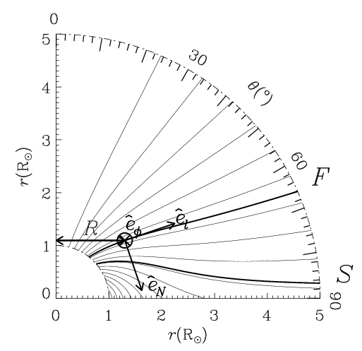
The background magnetic field configuration is depicted in Fig.1, where the thick contours labeled and represent the lines of force along which we examine the fast and slow solar wind solutions, respectively. Tube (), which intersects the Earth orbit at 70∘ (89∘) colatitude, originates from () at the Sun where the meridional magnetic field strength is () G.
3.2 Prescribed meridional flow profiles
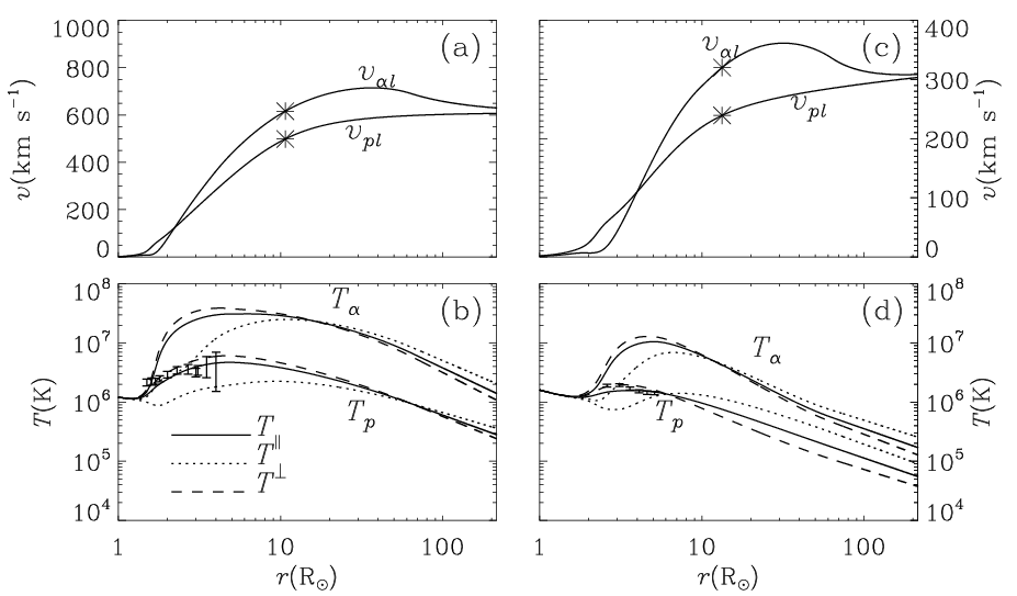
The background meridional flow parameters are found by adopting a three-step approach described as follows:
- 1.
Using some ad hoc heating parameters, we solve along flux tube () the isotropic version of Eqs.(22) to (25) (see Eqs.(8) to (10) in Li & Li (2007) for details) to yield the distribution between 1 and 1 AU of the ion number densities and meridional speeds (), as well as the isotropic species temperatures () for the fast (slow) solar wind. Specifically, the heating rates are of the same format as in section 3.2 in Li & Li (2008). To generate the fast and slow solar wind solutions, the parameters (in ), (in ), are chosen to be and , respectively. By simply adjusting the heating parameters it proves difficult to produce a reasonable profile in that if in the inner corona is close to observations then at 1 AU is usually only a fraction of the typically measured values. Moreover, the derived speed difference varies little between 0.3 and 1 AU, in contrast to the Helios measurements. Therefore some additional steps are employed to make the flow profiles more realistic. Specifically, all the parameters except and are required to undergo a smooth transition from the profiles for the region AU derived so far to those specified in next step for the outer region.
- 2.
The desired profiles, given in Table 1, for , and for the region AU (denoted by subscript ) are based on the in situ measurements to be detailed shortly. Once is known, the meridional alpha speed is given by , and the alpha density by , where the subscript denotes the values obtained in the first step. The distributions of , () and () thus constructed are for the isotropic model.
- 3.
Now the ion temperatures can be constructed by prescribing the temperature anisotropy (). Note that the electron temperature is assumed to be isotropic. For the region within several solar radii, is required to decrease with from at 1 , where the Coulomb self-collisions are still frequent enough to suppress a temperature anisotropy, to some value less than unity. This inner profile is not directly constrained by observations but constructed by noting that the processes operational in the inner corona tend to heat the ions preferentially in the perpendicular direction (Hollweg & Isenberg 2002, e.g.,). On the other hand, for AU, follows a power law dependence on with the exponent determined by the Helios measurements (see Table 1). Specifying the temperature anisotropies of protons and alpha particles at 1 AU, and , determines in the outer region. The inner and outer profiles are then connected smoothly to yield the desired . The temperatures follow from the relations and .
A detailed description of Table 1 is necessary. Note that throughout this table where AU. Let us first focus on the adopted values for the fast solar wind. For the isotropic proton and alpha temperatures at 1 AU, we adopted the typical values of K and (Schwenn 1990; McComas et al. 2000, see e.g.,) (hereafter Sch90 and Mc00). Furthermore, Figures 18 and 19 in Marsch et al. (1982b) (hereafter M82b) indicate that , and . A power law dependence for of is therefore consistent with such a behavior, and also consistent with the Ulysses measurements (see Table 2 in Mc00). Furthermore, Figure 5 in Marsch et al. (1982a) (hereafter M82a) indicates that , and . A profile of is consistent with this behavior, but differs substantially from that measured by Ulysses, which yields that (see Table 2 in Mc00). Moving on to the slow solar wind, we note that values of K and K are typically found at 1 AU (see e.g., Sch90). In addition, Figures 18 and 19 in M82b indicate that , and . Therefore we adopted a profile of . On the other hand, we adopted a profile for in the form , which is consistent with the measured alpha temperature anisotropies which indicate that , and (see Fig.5 in M82a).
In this study and will serve as free parameters. The Helios measurements indicate that and for the fast solar wind with , while and for the slow solar wind with (Marsch et al. 1982a; Marsch et al. 1982b). Theoretically, one may expect that the pair may not occupy the whole rectangle bounded by the given values in the - space, since too strong an anisotropy can drive the system unstable with respect to a number of instabilities when the plasma is comparable to unity. Given that the lower limit of or is only slightly lower than , the ion-cyclotron instability can be shown to be unlikely to occur (Gary et al. 1994, see, e.g., Eq.(3) in). However, the firehose instability may be relevant since it happens when is sufficiently larger than and . Note that the alpha particles with a non-negligible abundance drifting relative to protons may complicate the situation considerably given that in addition to the firehose, electromagnetic ion/ion instabilities may also be relevant and the occurrence of such instabilities is not restricted to the cases where the parallel is large (Hellinger & Trávníček 2006). Nevertheless, we only compare the modeled with the non-resonant firehose criterion such as found via the dispersion relation of Alfvén waves (Isenberg 1984, see Eq.(23) in). Specializing to an electron-proton-alpha plasma, the dispersion relation dictates that instability occurs when where () with being the Alfvén speed determined by the bulk mass density . Using this criterion it is found that the modeled flow profiles are all stable with the only exception being for the segment in the fast wind with the largest values of and .
Figure 2 gives the radial distributions between 1 and 1 AU of the flow parameters for the fast and slow solar wind in the left and right panels, respectively. Figures 2a and 2c depict the meridional ion speeds and , while the ion temperatures (the dotted curves), (dashed) and (solid) are given in Figs.2b and 2d (). The values for the temperature anisotropy adopted for the construction are and for the fast wind, and and for the slow wind. In Fig.2b, the error bars represent the uncertainties of the UVCS measurements for the proton effective temperature, made for a polar coronal hole as reported by Kohl et al. (1998). Similar measurements by Frazin et al. (2003) along the edges of an equatorial streamer are given in Fig.2d. Moreover, the asterisks in Figs.2a and 2c mark the location of the Alfvén point as defined by Eq.(18).
For the fast (slow) solar wind it is found that at 1 AU the meridional proton speed is () , the proton flux is () in units of , the alpha abundance is 4.56% (3.6%), and the meridional component of the proton-alpha velocity difference is 23 (5) . These values are consistent with in situ measurements such as made by Ulysses (McComas et al. 2000). Moreover, the fast (slow) solar wind reaches the Alfvén point at 10.7 (13.3) , beyond which increases only slightly with increasing . On the other hand, for AU the meridional alpha speed decreases rather than increases with as a consequence of the prescribed profile. If examining the ratio of to the meridional Alfvén speed , one may find that for the fast solar wind this ratio decreases only slightly from at 0.3 AU to at 1 AU, while for the slow wind it shows a substantial variation from at 0.3 AU to at 1 AU. The modeled can be seen to agree with the Helios measurements as given by Fig.11 of Marsch et al. (1982a). Note that a value of at 0.3 AU is not unrealistic for slow solar winds, even larger values have been found by Helios 2 when approaching perihelion (Marsch et al. 1981). Moving on to the temperature profiles, one may see that the profiles inside 5 are in reasonable agreement with the UVCS line-width measurements for both the fast and slow solar wind.
| fast wind | slow wind | |
|---|---|---|
| 11 1 please see section 3.2 for details | ||
| K | K | |
| K | K | |
4 Numerical results
Having described the meridional magnetic field and flow profiles, we may now address the following questions: to what extent is the total angular momentum loss of the Sun affected by the ion temperature anisotropies? and how is the angular momentum budget distributed among particle momenta, the magnetic torque, and the torque due to ion temperature anisotropies? To this end, let us first examine the fast and then the slow solar wind solutions. In the computations, we take rad s-1, which corresponds to a sidereal rotation period of days.
4.1 Fast solar wind
Figure 3 presents the radial profiles of (a) the proton azimuthal speed , (b) the alpha one , and (c) the ion angular momentum fluxes (), their sum , the flux due to the magnetic torque , and that due to temperature anisotropies (see Eq.(16)). Note that the dash-dotted curves in Fig.3c plot negative values. In Figs.3a and 3b, the ion azimuthal speeds for the isotropic model with identical meridional flow parameters are given by the dashed lines for comparison. The fast wind profile corresponds to and .
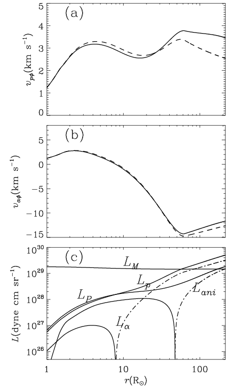
For the chosen and , it is found that . Consequently, the total angular momentum loss rate per steradian is (here and hereafter in units of ) in the anisotropic case, and is only modestly enhanced compared with the isotropic case, for which . Furthermore, Figs.3a and 3b indicate that the radial dependence of the ion azimuthal speed or in the anisotropic model is similar to that in the isotropic one. For instance, both models yield that with increasing distance the alpha particles develop an azimuthal speed in the direction of counterrotation with the Sun: becomes negative beyond () in the anisotropic (isotropic) model. The difference between the isotropic and anisotropic cases becomes more prominent at large distances where becomes increasingly significant, as would be expected from Eq.(17). Take the values of and at 1 AU. The isotropic (anisotropic) model yields that () and that () at 1 AU. Note that the changes introduced to the ion azimuthal speeds by pressure anisotropies ( for both protons and alpha particles) play an important role in the distribution of the angular momentum budget among different contributions, as shown by Fig.3c. The proton contribution exceeds for and attains at 1 AU, significantly larger than the magnetic part at the same location. In fact, the overall particle contribution , which increases with distance, overtakes the magnetic contribution from onwards, despite the fact that the alpha contribution tends to offset the proton one. The dominance of over happens in conjunction with the increasing importance of , the flux due to total pressure anisotropy which is in the direction of counterrotation with the Sun. In contrast, without pressure anisotropies, at 1 AU it turns out that even though a value of is found for , it is almost cancelled by an of . The resulting is thus , substantially smaller than , which is nearly identical to the value found in the anisotropic model. This contrast between anisotropic and isotropic cases is understandable since it follows from Eq.(13) that, given that the constant does not vary much from the isotropic to anisotropic model, the change of should be largely offset by that of .
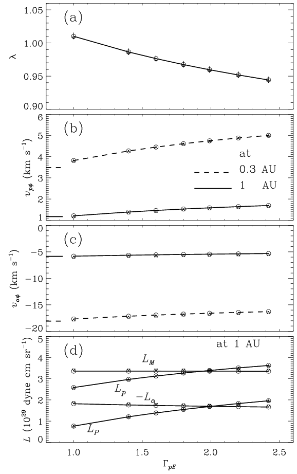
Figure 4 expands the obtained results by displaying the dependence on and of (a) the factor , (b) the proton azimuthal speed and (c) the alpha one at two different distances plotted by the different linestyles indicated in (b), as well as (d) the constituents comprising the angular momentum flux at 1 AU. In addition to the individual ion contributions and , and the magnetic one , the overall particle contribution is also given. Note that instead of is plotted in Fig.4d. Moreover, the horizontal bars on the left of Figs.4b and 4c represent the azimuthal ion speeds derived in the isotropic case at the corresponding locations for comparison. The open circles correspond to the cases where . It turns out that at any given each parameter varies monotonically from the value with , represented by the end of the arrow, to the value with given by the arrow head. In Fig.4b the arrows have been slightly shifted from one another to avoid overlapping.
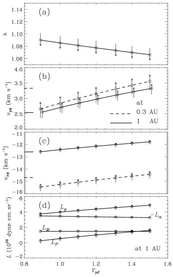
From Fig.4a one can see that decreases with increasing or , ranging from at the upper left to at the lower right corner. The deviation of from unity, albeit modest, indicates that the changes introduced in the total angular momentum loss due to the ion pressure anisotropies are not negligible. From Figs.4b and 4c one can see that between 0.3 to 1 AU, the magnitude of the azimuthal speeds of both species decreases with increasing distance. Furthermore, at either 0.3 or 1 AU, both and increase when or increases. Take the values at 1 AU for instance. One can see that ranges from to , while varies between and . For the majority of the solutions both and tend to be larger in the algebraic sense than the corresponding values in the isotropic model, which yield and for protons and alpha particles, respectively. However, at 0.3 AU or tends to be smaller in the anisotropic than in the isotropic case. Now and vary in the intervals and , respectively. For comparison, the isotropic model yields a () of () . Now let us examine the specific angular momentum fluxes , and at 1 AU. Figure 4d indicates that has the weakest parameter dependence, which is easily understandable given that to a good approximation where may be taken to be or (see Eq.(10)). Besides, the parameter dependence of is rather modest, varying by % from to when or changes. On the other hand, changes substantially, ranging between and . Hence the overall particle contribution also shows a significant parameter dependence. In particular, may exceed when . For the solutions examined, can be found to be positive and attain its maximum of when . Only for the lowest values of and can one find a negative of . Moreover, the protons always show a partial corotation, i.e., . From this we conclude that the ion temperature anisotropies are unlikely the cause of the tendency for or to be negative for the fast solar wind as indicated by the Helios measurements (Pizzo et al. 1983; Marsch & Richter 1984).
4.2 Slow solar wind
Figure 5 presents, in the same fashion as Fig.4, the dependence on and of various quantities derived for the slow solar wind. A comparison with Fig.4 indicates that nearly all the features in Fig.5 are reminiscent of those obtained for fast solar wind solutions. However, some quantitative differences exist nonetheless. For instance, when is held fixed, all the examined parameters for the slow wind vary little even though changes considerably from to . In contrast, the parameters for the fast wind show an obvious dependence. This difference can be largely attributed to the fact that in the slow wind the ions are substantially cooler than in the fast wind. Figure 5a shows that ranges from to . In other words, relative to the isotropic case, the solar angular momentum loss rate per steradian in the anisotropic models may be enhanced or reduced by up to . If examining Figs.5b and 5c, one may find that at both and AU, the azimuthal speeds of both ion species, and , are larger algebraically in the anisotropic models than in the isotropic one. The difference between the two is more prominent at 0.3 AU, where the isotropic model yields that , whereas the anisotropic models yield that with increasing , increases from to , and varies between to . As for the ion azimuthal speeds at 1 AU, one can see that varying leads to a varying between and , and a ranging from to . The corresponding changes in the specific ion angular momentum fluxes are shown by Fig.5d, which indicates that the proton one increases with increasing from to , and likewise, the alpha one increases from to . On the other hand, the flux associated with magnetic stresses hardly varies, and a value of can be quoted for all the models examined. Therefore in the parameter space explored, may be smaller than , which is however offset by the alpha contribution that is always in the direction of counter-rotation to the Sun. In fact, the alpha contribution is so significant that the overall particle contribution never exceeds . In other words, incorporating ion temperature anisotropy cannot resolve the outstanding discrepancy between previous models and observations concerning the relative importance of particle and magnetic contributions in the angular momentum budget of the solar wind.
5 Discussion
As demonstrated by Li & Li (2008), the discussion on the angular momentum transport also allows us to say a few words on the frequency spectra () of the ion velocity fluctuations during Alfvénic activities in the fast solar wind in the super-Alfvénic portion where . This is due to the well-known change of the properties of Alfvénic fluctuations around some , where is the speed of center of mass evaluated at the Alfvén point (Heinemann & Olbert 1980; Li & Li 2008, see e.g., ). For typical fast wind parameters, . While the fluctuations with frequencies are genuinely wave-like and may be described by the WKB limit given the slow spatial variation of flow parameters in the region in question, those with behave in a quasi-static manner and may be described by the solutions to the angular momentum conservation law which also governs the zero-frequency fluctuations. As shown by Li & Li (2008) who neglected the species temperature anisotropy, in the region AU which will be explored by the Solar Orbiter and Solar Probe, the ratio of the alpha to proton velocity fluctuation amplitude can be an order-of-magnitude larger for than for . Hence one may expect that, if the proton velocity fluctuation spectrum is somehow smooth around , then the alpha one will show an apparent spectral break. Now let us revisit this problem in light of the discussion presented in this paper and see what changes the pressure anisotropies may introduce.
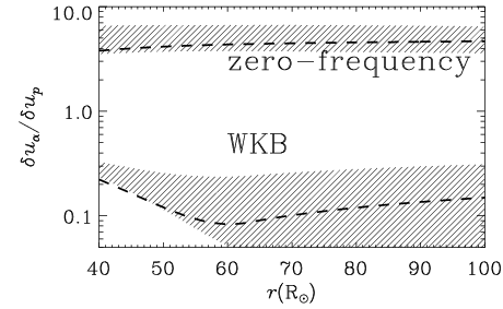
Restrict ourselves to either the high-latitude region or the region inside say such that the magnetic field may be seen as radial. Furthermore, suppose that the waves are propagating parallel to the magnetic field in the empirical fast wind profiles detailed in section 3. Figure 6 presents the radial dependence of in the region between and for both the zero-frequency (upper part) and WKB (lower part) solutions. For comparison, the dashed curves represent the corresponding results in the isotropic model. To construct Fig.6, all the possible values of and have been examined. As a result, at any radial location the ratio varies from model to model, and the range in which this ratio may occupy is given by the hatched area. The zero-frequency solutions are obtained by solving Eq.(20), while for hydromagnetic WKB Alfvén waves it is well known that , where is the wave phase speed and given by (Barnes & Suffolk 1971; Isenberg 1984, e.g.,)
in which is the speed of center of mass, and () defines the fractional ion mass density.
From Fig.6 one can see that the zero-frequency and WKB solutions are well separated from each other, in the isotropic and anisotropic cases alike. For the isotropic model, in the zero-frequency case increases monotonically from at 40 to 4.68 at 100 . On the other hand, in the WKB case it decreases first from 0.22 at 40 and attains its minimum of at and then increases to 0.15 at 100 . The difference in between the zero-frequency and WKB solutions may be slightly smaller in the anisotropic than in the isotropic case for some combinations of , but the difference is still quite significant. From this we can conclude that, with realistic ion temperature anisotropies included, the alpha velocity fluctuation spectrum during Alfvénic activities will also show an apparent break near , if the proton one is smooth there. This break is entirely a linear property, and has nothing to do with the nonlinearities that may also shape the fluctuation spectra.
6 Summary
This study has been motivated by the apparent lack of an analysis on the angular momentum transport in a multicomponent solar or stellar wind with differentially flowing ions and species temperature anisotropy. Moreover, there has been an outstanding discrepancy between available measurements and models concerning the relative importance of the particle and magnetic contribution to the solar angular momentum loss rate per steradian . The Helios measurements indicate that for fast (slow) solar wind with () , tends to be negative (positive), with the positive sign denoting the direction of corotation with the Sun. Furthermore, tends to be larger than in the slow wind. The behavior of derives from that of individual ion angular momentum fluxes, and , thereby calling for a multifluid approach.
Starting with a general set of multifluid transport equations with gyrotropic species pressure tensors, we have derived the equations for both the angular momentum conservation (Eqs.(10) and (20) in section 2), and the energy and linear momentum balance (Eqs.(22) to (25) in the appendix). These equations are not restricted to radial outflows in the equatorial plane, instead they are valid for arbitrary axisymmetrical winds that include two major ion species, and therefore are expected to find applications in general outflows from late-type stars. To focus on the problem of angular momentum transport, we refrained from solving the full set of equations governing the meridional dynamics. Rather, we constructed, largely based on the available in situ measurements, the empirical profiles for the meridional magnetic field and flow parameters. Only the ion temperature anisotropies are considered, i.e., the electron temperature is seen as isotropic. For both the fast and slow solar wind profiles, we solved the angular momentum conservation law (Eqs.(10) and (20)) to examine how the azimuthal speeds of protons and alpha particles , as well as the individual components in the solar angular momentum budget are influenced by the ion temperature anisotropies. To this end, solutions to the isotropic version are obtained for comparison.
Our main conclusions are:
- 1.
From the derived equations governing the energy transport, a simple analysis given in the appendix yields that the adiabatic cooling may be considerably influenced with the introduction of the azimuthal components. Such an influence is understandably more prominent in the low-latitude regions. This means, when modeling the species temperature anisotropy, for a quantitative comparison of model computations to be made with the near-ecliptic measurements such as made by Helios, the spiral magnetic field has to be taken into account.
- 2.
In agreement with the single-fluid case (Weber & Davis 1970; Weber 1970), incorporating species temperature anisotropy leads to a situation where the total angular momentum loss rate per steradian is determined by the behavior of the solution to the angular momentum conservation law in the vicinity of the Alfvén point where the combined Alfvénic Mach number . However, has to take into account the contribution from both ion species, as defined by Eq.(18).
- 3.
Relative to the isotropic case, the introduced species temperature anisotropy may enhance or decrease by up to %, and introduce an absolute change of up to in individual ion azimuthal speeds in the region between and AU. While these changes seem modest, the corresponding changes in the angular momentum fluxes convected by protons or alpha particles may change substantially. In contrast, the flux associated with magnetic stresses hardly varies.
- 4.
However, introducing ion temperature anisotropies cannot resolve the discrepancy between in situ measurements and models. For the fast wind solutions, while in extreme cases may become negative always stays positive. On the other hand, for the slow solar wind solutions examined, never exceeds even though may be smaller than the individual ion contribution. This is because, for both the slow and fast wind solutions, and always have opposite signs.
- 5.
The discussion on the angular momentum transport has some bearing on the ion velocity fluctuation spectra () during Alfvénic activities in the super-Alfvénic regions, which are likely to be explored by future missions such as Solar Orbiter and Solar Probe. In agreement with Li & Li (2008) where species temperature anisotropies are neglected, an analysis based on the WKB and zero-frequency solutions yields that will show an apparent break around some critical frequency if is smooth there. This is the well-known frequency that separates the genuinely wave-like fluctuations from quasi-static ones.
Acknowledgements.
We thank the referee (Dr. Horst Fichtner) for his very helpful comments. This research is supported by an STFC rolling grant to Aberystwyth University.References
- Banaszkiewicz et al. (1998) Banaszkiewicz, M., Axford, W. I., & McKenzie, J. F. 1998, A&A, 337, 940
- Barakat & Schunk (1982) Barakat, A. R., & Schunk, R. W. 1982, Plasma Phys., 24, 389
- Barnes & Suffolk (1971) Barnes, A., & Suffolk, G. C. J. 1971, J. Plasma Phys., 5, 315
- Belcher & MacGregor (1976) Belcher, J. W., & MacGregor, K. B. 1976, ApJ, 210, 498
- Bouvier et al. (1997) Bouvier, J., Forestini, M., & Allain, S. 1997 A&A, 326, 1023
- Frazin et al. (2003) Frazin, R. A., Cranmer, S. R., & Kohl, J. L. 2003, ApJ, 597, 1145
- Gary et al. (1994) Gary, S. P., McKean, M. E., Winske, D., Anderson, B. J., Denton, R. E., & Fuselier, S. A. 1994, J. Geophys. Res., 99, 5903
- Heinemann & Olbert (1980) Heinemann, M. & Olbert, S. 1980, J. Geophys. Res., 85, 1311
- Hellinger & Trávníček (2006) Hellinger, P., & Trávníček, P. 2006, J. Geophys. Res., 111, A01107, doi:10.1029/2005JA011318
- Hollweg & Isenberg (2002) Hollweg, J. V., & Isenberg, P. A. 2002, J. Geophys. Res., 107(A7), 1147, doi:10.1029/2001JA000270
- Hu & Habbal (1999) Hu, Y. Q., & Habbal, S. R. 1999, J. Geophys. Res., 104, 17045
- Isenberg (1984) Isernberg, P. A. 1984, J. Geophys. Res., 89, 6613
- Kohl et al. (1998) Kohl, J. L., Noci, G., Antonucci, E. et al. 1998, ApJ, 501, L127
- Leer & Axford (1972) Leer, E., & Axford, W. I. 1972, Sol. Phys., 23, 238
- Li et al. (2006) Li, B., Li, X., & Labrosse, N. 2006, J. Geophys. Res., 111, A08106, doi:10.1029/2005JA011303
- Li et al. (2007) Li, B., Habbal, S. R., & Li, X. 2007, ApJ, 661, 593
- Li & Li (2006) Li, B., & Li, X. 2006, A&A, 456, 359
- Li & Li (2007) Li, B., & Li, X. 2007, ApJ, 661, 1222
- Li & Li (2008) Li, B., & Li, X. 2008, ApJ, 682, 667
- Marsch et al. (1981) Marsch, E., Mühlhäuser, K.-H., Rosenbauer, H., Schwenn, R., & Denskat, K. U. 1981, J. Geophys. Res., 86, 9199
- Marsch et al. (1982a) Marsch, E., Mühlhäuser, K.-H., Rosenbauer, H., Schwenn, R., & Neubauer, F. M. 1982a, J. Geophys. Res., 87, 35 (M82a)
- Marsch et al. (1982b) Marsch, E., Mühlhäuser, K.-H., Schwenn, R., Rosenbauer, H., Pilipp, W., & Neubauer, F. M. 1982b, J. Geophys. Res., 87, 52 (M82b)
- Marsch & Richter (1984) Marsch, E., & Richter, A. K. 1984, J. Geophys. Res., 89, 5386
- McComas et al. (2000) McComas, D. J., Barraclough, B. L., Funsten, H. O., et al. 2000, J. Geophys. Res., 105, 10419 (Mc00)
- McKenzie et al. (1979) McKenzie, J. F., Ip, W.-H., & Axford, W. I. 1979, Ap&SS, 64, 183
- Mestel & Spruit (1987) Mestel, L., & Spruit, H. C. 1987, MNRAS, 226, 57
- Pizzo et al. (1983) Pizzo, V., Schwenn, R., Marsch, E. et al. 1983, ApJ, 271, 335
- Pneuman & Kopp (1971) Pneuman, G. W., & Kopp, R. A. 1971, Sol. Phys., 18, 258
- Sakurai (1985) Sakurai, T. 1985, A&A, 152, 121
- Scherer et al. (2001) Scherer, K., Marsch, E., Schwenn, R., & Rosenbauer, H. 2001, A&A, 366, 331
- Schwenn (1990) Schwenn, R. 1990, Large-scale structure of the interplanetary medium, in Physics of the Inner Heliosphere I, Large Scale Phenomena, eds. R. Schwenn, & E. Marsch (Springer-Verlag, New York), 99 (Sch90)
- Smith & Balogh (1995) Smith, E. J., & Balogh, A. 1995, Geochim. Res. Lett., 22, 3317
- Weber (1970) Weber, E. J. 1970, Sol. Phys., 13, 240
- Weber & Davis (1967) Weber, E. J., & Davis, Jr., L. 1967, ApJ, 148, 217
- Weber & Davis (1970) Weber, E. J., & Davis, Jr., L. 1970, J. Geophys. Res., 75, 2419
Appendix A Derivation of equations governing the meridional dynamics
In section 2, we have demonstrated that the vector equations governing a time-independent multicomponent solar wind with species temperature anisotropy are allowed to be decomposed into a force balance condition across the poloidal magnetic field and a set of transport equations along it. The azimuthal dynamics has been discussed in the text, whereas this appendix provides some discussion on the poloidal dynamics. In particular, we shall derive the equations governing the poloidal motion of ion species (), and the species temperatures () in rather general situations.
Due to the presence of in the component of the ion momentum equation (2), one may expect that the -component of Eq.(2) has to be solved. In fact, there is no need to do so because appears only in the difference , which may be found from the component of Eq.(2). Substituting into the component of Eq.(2) will then eliminate the cumbersome and . Note that this technique, first devised by McKenzie et al. (1979), ensures the conservation of not only total momentum but also total energy (Li & Li 2006, see). Specifically, the resulting equations for the poloidal dynamics are
| (22) | |||||
| (23) | |||||
| (24) | |||||
| (25) |
where (), results from Coulomb frictions, and the prime ′ represents the derivative with respect to the arclength . When deriving Eqs.(24) and (25), we have used the fact that the expression
may be simplified by expressing via the alignment condition (10), the result being
Similarly, one may find that
Now let us compare these equations with those in Isenberg (1984). It is straightforward to show that Eqs.(24) and (25) are equivalent to Eqs.(A3) and (A4) in Isenberg (1984) by specializing to a spherically symmetric solar wind and by noting that . On the other hand, using the alignment condition (10) one may find that
| (26) | |||||
Again specializing to a spherical solar wind, one then finds that Eq.(23) is equivalent to (A2) in Isenberg (1984). It should be stressed that although working in a frame of reference corotating with the Sun, as did Isenberg (1984), substantially simplifies the algebra, it does not offer the information on the specific form of the spiral angle , whose functional dependence on the flow speeds has to be assumed a priori. In practice, Isenberg (1984) assumed that the velocity of center of mass is radial in an inertial frame beyond 10 , which is certainly a good assumption for the present slow-rotating Sun. However, from our discussion on the azimuthal dynamics, there is in general no guarantee that is radial, and the deviation may be substantial for winds that flow from a faster rotating star.
Introducing azimuthal components may influence the ion flow speeds both directly and indirectly. The direct consequence is that azimuthal components may introduce into the reduced meridional momentum equation (23) an effective force (see the first three terms). Note that in a corotating frame the magnitude of the ion velocity becomes , from relation (26) one may see that in such a frame all particles move in the same centrifugal potential . Therefore in effect the introduced force tends to reduce the magnitude of the ion speed difference with increasing distance as tends to increase. This effect has been explored in detail in Li & Li (2006) and Li et al. (2007), where it is shown that the influence may play an important part in the force balance for the solar wind. In fact, introducing solar rotation alone is able to reproduce the profile measured by Ulysses beyond 2 AU if a proper value of is imposed there. On the other hand, may be altered indirectly by the modified pressure gradient force due to changes in the temperatures, which in turn are caused by the changes in the heat fluxes (the third term in Eqs.(24) and (25)) and through the adiabatic cooling (the second term). A detailed discussion on the former requires a specific form for the heat flux, which is beyond the scope of the present paper. As a consequence, we shall focus on the latter instead.
Neglecting the terms in the second pair of square parentheses, Eqs.(24) and (25) give
| (27) |
Note that the relation governing simply reflects the conservation of magnetic moment. Now that in the region say is significant and increases with , () may be substantially reduced (enhanced) relative to the case where . This effect is particularly significant in the near-ecliptic region and for the slow solar wind. For instance, restrict ourselves to the equatorial plane and consider the region between say 10 and 1 AU. Suppose remains constant and km/s. Now that roughly speaking , when the spiral field is considered, () at 1 AU is () times the value for a purely radial magnetic field. This suggests that for making any quantitative comparison of the modeled species temperature anisotropy with the near-ecliptic measurements such as made by Helios, the spiral magnetic field has to be considered.
For completeness, we note that the force balance condition across the direction comes from the component of the total momentum, which reads
| (28) | |||||
where is the signed curvature radius of the poloidal magnetic line of force. Obviously, this force balance condition determines the poloidal magnetic field configuration in response to the electric currents associated with the flow. This equation, combined with the transport equations along the meridional magnetic line of force, may be solved alternately to find a self-consistent solution to the vector equations by using the approach by Pneuman & Kopp (1971) or Sakurai (1985).