Polymorphic evolution sequence and evolutionary branching

Nicolas Champagnat ^†^†thanks: EPI TOSCA, INRIA Sophia Antipolis – Méditerranée, 2004 route des Lucioles, BP. 93, 06902 Sophia Antipolis Cedex, France; e-mail: Nicolas.Champagnat@sophia.inria.fr. Sylvie Méléard ^†^†thanks: CMAP, Ecole Polytechnique, CNRS, route de Saclay, 91128 Palaiseau Cedex-France; e-mail: sylvie.meleard@polytechnique.edu.

August 24, 2026

Abstract

We are interested in the study of models describing the evolution of a polymorphic population with mutation and selection in the specific scales of the biological framework of adaptive dynamics. The population size is assumed to be large and the mutation rate small. We prove that under a good combination of these two scales, the population process is approximated in the long time scale of mutations by a Markov pure jump process describing the successive trait equilibria of the population. This process, which generalizes the so-called trait substitution sequence, is called polymorphic evolution sequence. Then we introduce a scaling of the size of mutations and we study the polymorphic evolution sequence in the limit of small mutations. From this study in the neighborhood of evolutionary singularities, we obtain a full mathematical justification of a heuristic criterion for the phenomenon of evolutionary branching. To this end we finely analyze the asymptotic behavior of 3-dimensional competitive Lotka-Volterra systems.

MSC 2000 subject classification: 92D25, 60J80, 37N25, 92D15, 60J75

Key-words: Mutation-selection individual-based model, fitness of invasion, adaptive dynamics, polymorphic evolution sequence, competitive Lotka-Volterra system, evolutionary branching.

1 Introduction

We consider an asexual population in which each individual’s ability to survive and reproduce is characterized by a quantitative trait, such as the size, the age at maturity, or the rate of food intake. Evolution, acting on the trait distribution of the population, is the consequence of three basic mechanisms: heredity, which transmits traits to new offsprings, mutation, driving a variation in the trait values in the population, and selection between these different trait values, which is due to the competition between individuals for limited resources or area. Adaptive dynamics models aim at studying the interplay between these different mechanisms [21, 25, 27]. Our approach is based on a microscopic individual-based model that details the ecological dynamics of each individual. From the simulated dynamics of this process initially issued from a monomorphic population, we observe that it is essentially single-modal centered around a trait that evolves continuously, until some time where the population divides into two separate sub-populations that are still in interaction but are centered around distinct traits at a distance increasing with time. This phenomenon, called Evolutionary Branching, is thought to be a possible explanation of phenotypic separation without geographic separation [7]. (One speaks about sympatric speciation though the population is asexual). Our aim in this paper is to understand the dynamics of the process in long time scales and to highlight the evolutionary branching phenomenon. In particular, we want to prove the conjecture stated by Metz et al. [26] and giving conditions on the parameters of the model allowing one to predict whether evolutionary branching will occur or not.

To this aim, we follow the basic description of adaptive dynamics based on the biologically motivated assumptions of rare mutations and large population. Under these assumptions, we prove that the microscopic process describing the ecological dynamics can be approximated by a Markov pure jump process on the set of point measures on the trait space. The transitions of this process are given by the long time behavior of competitive Lotka-Volterra systems. They describe the succession of mutant invasions followed by a fast competition phase between the mutant population and the resident one. In the mutation time scale, and for large populations, the successful traits in the competition are given by the nontrivial equilibria of Lotka-Volterra systems which model the dynamics of the sizes of each sub-population corresponding to each resident or mutant trait. We thus generalize the situation introduced in [26] and mathematically developed in [4], where the parameters of the model prevent the coexistence of two traits. In that case, the microscopic model converges to a monomorphic (one trait support) pure jump process, called Trait Substitution Sequence (TSS). This limit involves a timescale separation between the mutations and the population dynamics driving the competition between traits.

In this article, we relax the assumption of non-coexistence and obtain a polymorphic evolution sequence (PES), allowing coexistence of several traits in the population, from the same microscopic model described in Section 2. In Section 2.3, we introduce the competitive symmetric Lotka-Volterra systems describing the competition between traits. We prove in Section 2.4 that the PES takes the form of a Markov jump process on the set of measures on the trait space ${\cal X}$ that are finite sums of Dirac masses with positive weights, and we characterize the transitions of this process in terms of the long time behaviour of competitive Lotka-Volterra systems. In Section 3, we explain why the assumptions ensuring the convergence to the PES are satisfied as long as no more than two traits coexist. In this case, the dynamics of the PES can be explicitely characterized. Next (Section 4), we study the transition from a monomorphic population to a stable dimorphic population, and give a full mathematical justification of the criterion for evolutionary branching proposed in [26], under the assumption of small mutation effects. To this end, we first show in Sections 4.1 and 4.2 that, away from evolutionary singularities, the support of the PES stays monorphic and converges to an ODE known as the “canonical equation” [8]. Finally, in Section 4.3, we characterize the situations where evolutionary branching occurs by specializing to our situation the results of Zeeman [30] on the asymptotic behavior of 3-dimensional competitive Lotka-Volterra systems.

Let us insist on the importance of the limits. Here we are concerned by the combination of the limits of large populations and rare mutations, followed by a limit of small mutations. An alternative approach would be first to study the limit of large population alone, giving in the limit an integro-differential partial differential equation for the density of traits [5]; and next to study a limit of small mutations on this equation with a proper time scaling that would lead to some dynamics on the set of finite sums of Dirac masses on the trait space. The second part of this program has already been partly studied in [9] in a specific model, but is related to difficult problems on Hamilton-Jacobi equations with constraints [2]. In this case, evolutionary branching is numerically observed, but not yet fully justified. Another approach would be to combine the three limits we consider directly at the level of the microscopic model, allowing one to study the evolutionary process on several time scales [3]. This requires a finer analysis of the invasion and competition phases after the appearance of a new mutant. Note that all these approaches are based on the same idea of separation between the time scales of mutation and competition.

2 Models and Polymorphic Evolution Sequence (PES)

Let us introduce here the main models on which our approach is based.

2.1 The individual-based model

The microscopic model we use is an individual-based model with density-dependence, which has been already studied in ecological or evolutionary contexts by many authors [12, 5].

The trait space ${\cal X}$ is assumed to be a compact subset of $\mathbb{R}^{l}$ , $l\geq 1$ . For any $x,y\in{\cal X}$ , we introduce the following biological parameters

$\lambda(x)\in\mathbb{R}_{+}$: is the rate of birth from an individual holding trait $x$ .
$\mu(x)\in\mathbb{R}_{+}$: is the rate of “natural” death for an individual holding trait $x$ .
$r(x):=\lambda(x)-\mu(x)$: is the “natural” growth rate of trait $x$ .
$K\in\mathbb{N}$: is a parameter scaling the population size and the resources.
${\alpha(x,y)\over K}\in\mathbb{R}_{+}$: is the competition kernel representing the pressure felt by an individual holding trait $x$ from an individual holding trait $y$ . It is not assumed to be a symmetric function.
$u_{K}\,p(x)$: with $u_{K},p(x)\in(0,1]$ , is the probability that a mutation occurs in a birth from an individual with trait $x$ . Small $u_{K}$ means rare mutations.
$m(x,h)dh$: is the law of $h=y-x$ , where the mutant trait $y$ is born from an individual with trait $x$ . Its support is a subset of ${\cal X}-x=\{y-x:y\in{\cal X}\}$ .

We consider, at any time $t\geq 0$ , a finite number $N_{t}$ of individuals, each of them holding a trait value in ${\cal X}$ . Let us denote by $x_{1},\ldots,x_{N_{t}}$ the trait values of these individuals. The state of the population at time $t\geq 0$ , rescaled by $K$ , is described by the finite point measure on ${\cal X}$

\nu^{K}_{t}=\frac{1}{K}\sum_{i=1}^{N_{t}}\delta_{x_{i}},

(2.1)

where $\delta_{x}$ is the Dirac measure at $x$ . Let $\>\langle\nu,f\rangle$ denote the integral of the measurable function $f$ with respect to the measure $\nu$ and $\mbox{Supp}(\nu)$ denote its support.

Then $\>\langle\nu^{K}_{t},{\bf 1}\rangle=\frac{N_{t}}{K}$ and for any $x\in{\cal X}$ , the positive number $\langle\nu^{K}_{t},{\bf 1}_{\{x\}}\rangle$ is called the density at time $t$ of trait $x$ .

Let ${\cal M}_{F}$ denote the set of finite nonnegative measures on ${\cal X}$ , equipped with the weak topology, and define

{\cal M}^{K}=\left\{\frac{1}{K}\sum_{i=1}^{n}\delta_{x_{i}}:n\geq 0,\ x_{1},\ldots,x_{n}\in{\cal X}\right\}.

An individual holding trait $x$ in the population $\nu^{K}_{t}$ gives birth to another individual with rate $\lambda(x)$ and dies with rate

\mu(x)+\int\alpha(x,y)\nu^{K}_{t}(dy)=\mu(x)+\frac{1}{K}\sum_{i=1}^{N_{t}}\alpha(x,x_{i}).

The parameter $K$ scales the strength of competition, thus allowing the coexistence of more individuals in the population. A newborn holds the same trait value as its progenitor with probability $1-u_{K}p(x)$ , and with probability $u_{K}p(x)$ , the newborn is a mutant whose trait value $y$ is chosen according to $y=x+h$ , where $h$ is a random variable with law $m(x,h)dh$ . In other words, the process $(\nu^{K}_{t},t\geq 0)$ is a ${\cal M}^{K}$ -valued Markov process with infinitesimal generator defined for any bounded measurable functions $\phi$ from ${\cal M}^{K}$ to $\mathbb{R}$ by

$\displaystyle L^{K}\phi(\nu)$	$\displaystyle=\int_{\cal X}\left(\phi\left(\nu+\frac{\delta_{x}}{K}\right)-\phi(\nu)\right)(1-u_{K}p(x))\lambda(x)K\nu(dx)$
	$\displaystyle+\int_{\cal X}\int_{\mathbb{R}^{l}}\left(\phi\left(\nu+\frac{\delta_{x+h}}{K}\right)-\phi(\nu)\right)u_{K}p(x)\lambda(x)m(x,h)dhK\nu(dx)$
	$\displaystyle+\int_{\cal X}\left(\phi\left(\nu-\frac{\delta_{x}}{K}\right)-\phi(\nu)\right)\left(\mu(x)+\int_{\cal X}\alpha(x,y)\nu(dy)\right)K\nu(dx).$	(2.2)

For $\nu\in{\cal M}^{K}$ , the integrals with respect to $K\nu(dx)$ in (2.2) correspond to sums over all individuals in the population. The first term (linear) describes the births without mutation, the second term (linear) describes the births with mutation, and the third term (non-linear) describes the deaths by oldness or competition. The density-dependent non-linearity of the third term models the competition in the population, and hence drives the selection process.

Let us denote by (A) the following three assumptions

(A1)

$\lambda$ , $\mu$ and $\alpha$ are measurable functions, and there exist $\bar{\lambda},\bar{\mu},\bar{\alpha}<+\infty$ such that

\lambda(\cdot)\leq\bar{\lambda},\quad\mu(\cdot)\leq\bar{\mu}\quad\mbox{and}\quad\alpha(\cdot,\cdot)\leq\bar{\alpha}.

(A2)

$r(x)=\lambda(x)-\mu(x)>0$ for any $x\in{\cal X}$ , and there exists $\underline{\alpha}>0$ such that $\ \underline{\alpha}\leq\alpha(\cdot,\cdot)$ .

(A3)

There exists a function $\bar{m}:\mathbb{R}^{l}\rightarrow\mathbb{R}_{+}$ such that $m(x,h)\leq\bar{m}(h)$ for any $x\in{\cal X}$ and $h\in\mathbb{R}^{l}$ , and $\int\bar{m}(h)dh<\infty$ .

For fixed $K$ , under (A1) and (A3) and assuming that $\mathbf{E}(\langle\nu^{K}_{0},\mathbf{1}\rangle)<\infty$ , the existence and uniqueness in law of a process on $\mathbb{D}(\mathbb{R}_{+},{\cal M}^{K})$ with infinitesimal generator $L^{K}$ has been proved in [12]. Assumption (A2) prevents the population to explode and to go extinct too fast.

2.2 An example

The birth-death-competition-mutation process described above has been heuristically studied in various ecological or evolutionary contexts. Let us illustrate the phenomenon of evolutionary branching we are interested in with a simple example, adapted from a classical model (Roughgarden [29], Dieckmann and Doebeli [7]). In this model, there is a single optimal trait value for the birth rate and a symmetric competition kernel. The parameters are the following:

\begin{gathered}{\cal X}=[-2,2];\quad\mu(x)\equiv 0;\quad p(x)\equiv p,\\ \lambda(x)=\exp(-x^{2}/2\sigma_{b}^{2}),\\ \alpha(x,y)=\tilde{\alpha}(x-y)=\exp(-(x-y)^{2}/2\sigma^{2}_{\alpha}).\end{gathered}

(2.3)

and $m(x,h)dh$ is the law of a ${\cal N}(0,\sigma^{2})$ r.v. $Y$ (centered Gaussian with variance $\sigma^{2}$ ) conditioned on $x+Y\in{\cal X}$ .

The growth rate $\lambda(x)$ is maximal at $x=0$ and there is local competition between traits, in the sense that $\alpha(x,y)$ is maximal for $x=y$ and is close to 0 when $|x-y|$ is large. If the competition kernel was flat ( $\alpha\equiv 1$ ), evolution would favor mutant traits with maximal growth rate. However, if competition is local, numerical simulations of the microscopic model give different patterns, as shown in Fig. 2.1. The pattern of Fig. 2.1(b), where the population, initially composed of traits concentrated around a single trait value, is driven by the evolutionary forces to states where the population is composed of two (or more) groups, concentrated around different trait values. This phenomenon is called evolutionary branching and has been observed in many biological models (see e.g. [26, 24, 17]). It is believed to be a possible mechanism of traits separation that could lead to speciation [7].

In this particular model, the possibility of evolutionary branching seems to be governed by the values of $\sigma_{b}$ and $\sigma_{\alpha}$ , which represent respectively the width of the trait region with high growth rate and the interaction range. In Fig. 2.1(a), $\sigma_{\alpha}>\sigma_{b}$ and there is no evolutionary branching, whereas in Fig. 2.1(b), $\sigma_{\alpha}<\sigma_{b}$ and evolutionary branching occurs. We observe in both simulations that, in a first phase, the population trait support is concentrated around a mean trait value that converges to 0. In a second phase, new mutants feel two different selective pressures: high growth rate (traits close to 0) and competition (traits far from the rest of the population). If $\sigma_{\alpha}$ is small, the selection pressure is weaker for traits away from 0 and allows the apparition of new branches. The goal of this article is to justify mathematically this heuristics.

Refer to caption — (a) $p=0.1$ , $K=1000$ , $\sigma=0.01$ , $\sigma_{b}=0.9$ , $\sigma_{\alpha}=1.0$ .

2.3 On scales

In order to analyze the phenomenon of evolutionary branching, we are going to consider three biological asymptotics in the individual-based model: large population ( $K\rightarrow+\infty$ ), rare mutations ( $u_{K}\rightarrow 0$ ) and small mutation amplitude. The combination of the two first scales will allow us to describe the polymorphic evolution sequence, we will focus on. This limit amounts to approximate the simulated dynamics of Fig. 2.1(a) and (b) of the previous section by the one of Fig. 2.2(a) and (b), respectively.

These scales and the biological heuristics of this approach were introduced in [26]. The main interest of the assumption of rare mutations is the separation between ecological and evolutionary time scales: the selection process has sufficient time between two mutations to eliminate disadvantaged traits. Then evolution proceeds by a succession of phases of mutant invasion and phases of competition between traits. We will choose parameters such that the ecological and evolutionary time scales are separated, leading to an evolutionary dynamics where competition phases are infinitesimal on the mutation time scale. In addition, the large population assumption allows one to assume a deterministic population dynamics between mutations, so that the outcome of the competition can be predicted. More formally, between two mutations, a finite number of traits are present, namely $x_{1},\ldots,x_{d}$ , and the population dynamics can be reduced to a Markov process in $\mathbb{N}^{d}$ .

Assume that, for all $i\in\{1,\ldots,d\}$ , $\frac{1}{K}\langle\nu^{K}_{0},\mathbf{1}_{\{x_{i}\}}\rangle$ has bounded second-order moments and converge in distribution to $n_{i}(0)\in\mathbb{R}_{+}$ . Then, as proved in [6, Thm.4.2], when $K\rightarrow+\infty$ , the process $\frac{1}{K}(\langle\nu^{K}_{t},\textbf{1}_{\{x_{1}\}}\rangle,\ldots,\langle\nu^{K}_{t},\textbf{1}_{\{x_{d}\}}\rangle)$ converges in distribution for the Skorohod topology to the solution of the $d$ -dimensional competitive Lotka-Volterra system $LV(d,\mathbf{x})$ with initial condition $(n_{1}(0),\ldots,n_{d}(0))$ .

Definition 2.1

For any $\mathbf{x}=(x_{1},\ldots,x_{d})\in{\cal X}^{d}$ , we denote by $LV(d,\mathbf{x})$ the competitive Lotka-Volterra system defined by

\dot{\mathbf{n}}(t)=F^{\mathbf{x}}(\mathbf{n}(t)),\quad 1\leq i\leq d,\quad t\geq 0,

(2.4)

where $\mathbf{n}(t)=(n_{1}(t),\ldots,n_{d}(t))$ ,

F^{\mathbf{x}}_{i}(\mathbf{n}):=n_{i}G^{\mathbf{x}}_{i}(\mathbf{n})\quad\hbox{ where }\quad G_{i}^{\mathbf{x}}(\mathbf{n}):=r(x_{i})-\sum_{j=1}^{d}\alpha(x_{i},x_{j})n_{j}.

(2.5)

The equilibria of $LV(d,\mathbf{x})$ are given by the intersection of hyperplanes $(P_{i})_{1\leq i\leq d}$ , where $P_{i}$ has equation either $n_{i}=0$ or $G_{i}^{\mathbf{x}}(\mathbf{n})=0$ . We need to introduce the following notion of coexisting traits.

Definition 2.2

For any $d\geq 0$ , we say that $x_{1},\ldots,x_{d}$ coexist if $LV(d,\mathbf{x})$ admits a unique non-trivial equilibrium $\bar{\mathbf{n}}(\mathbf{x})\in({\mathbb{R}}_{+}^{*})^{d}$ locally strongly stable, in the sense that the eigenvalues of the Jacobian matrix of $LV(d,\mathbf{x})$ at $\bar{\mathbf{n}}(\mathbf{x})$ have all (strictly) negative real part. In particular, for all $i\in\{1,\ldots,d\}$ ,

G_{i}^{\mathbf{x}}(\bar{\mathbf{n}}(\mathbf{x}))=0\quad\hbox{ and }\quad DF^{\mathbf{x}}(\bar{\mathbf{n}}(\mathbf{x}))=((-\alpha(x_{i},x_{j})\bar{\mathbf{n}}_{i}(\mathbf{x})))_{1\leq i,j\leq d}.

(2.6)

In the monomorphic case ( $d=1$ ) and when $r(x)>0$ , the competitive Lotka-Volterra system $LV(1,x)$ takes the form of the so-called logistic equation

\dot{n}_{x}=n_{x}(r(x)-\alpha(x,x)n_{x}).

(2.7)

The unique stable equilibrium of this equation is $\bar{n}(x)=r(x)/\alpha(x,x)$ .

Similarly, in the dimorphic case where $d=2$ , the system $LV(2,(x,y))$ takes the form

\begin{cases}\dot{n}_{x}=n_{x}(r(x)-\alpha(x,x)n_{x}-\alpha(x,y)n_{y})\\ \dot{n}_{y}=n_{y}(r(y)-\alpha(y,x)n_{x}-\alpha(y,y)n_{y}).\end{cases}

(2.8)

Under Assumption (A2), the equilibria of (2.8) are $(0,0)$ , $(\bar{n}(x),0)$ , $(0,\bar{n}(y))$ and possibly a non-trivial equilibrium in $(\mathbb{R}_{+}^{*})^{2}$ . It is known (see e.g. [22]) that the non trivial equilibrium exists and is locally strongly stable, (traits $x$ and $y$ coexist), if and only if $f(x;y)>0$ and $f(y;x)>0$ , where

f(y;x)=r(y)-\alpha(y,x)\bar{n}(x).

(2.9)

2.4 Convergence to the Polymorphic Evolution Sequence (PES)

Our goal here is to examine the asymptotic behavior of the microscopic process when the population size grows to infinity as well as the mutation rate converges to 0, in a long time scale. Before stating our convergence result, we first give an idea of the argument used, extending the biological heuristics of [26] and the special case of the trait substitution sequence (TSS) developed in [4] (see also Section 3.1).

2.4.1 Idea of the proof

Let us roughly describe the successive steps of mutation, invasion and competition. The two steps of the invasion of a mutant in a given population are firstly the stabilization of the resident population before the mutation and secondly the invasion of the mutant population after the mutation.

Fix $\eta>0$ . In the first step, assuming that $d$ traits $x_{1},\ldots,x_{d}$ that coexist are present, we prove that the population densities $(\langle\nu^{K}_{t},\mathbf{1}_{\{x_{1}\}}\rangle,\ldots,\langle\nu^{K}_{t},\mathbf{1}_{\{x_{d}\}}\rangle)$ belong to the $\eta$ -neighborhood of $\bar{\mathbf{n}}(\mathbf{x})$ with high probability for large $K$ until the next mutant $y$ appears. To this aim, we use large deviation results on the problem of exit from a domain [13] to prove that the time needed for the population densities to leave the $\eta$ -neighborhood of $\bar{\mathbf{n}}(\mathbf{x})$ is bigger than $\exp(VK)$ for some $V>0$ with high probability. Therefore, until this exit time, the rate of mutation from trait $x_{i}$ in the population is close to $u_{K}p(x_{i})\lambda(x_{i})K\bar{n}_{i}(\mathbf{x})$ and thus, the first mutation appears before this exit time if one assumes that

\frac{1}{Ku_{K}}\ll e^{VK}.

In particular, the mutation rate from trait $x_{i}$ on the time scale $t/Ku_{K}$ is close to

p(x_{i})\lambda(x_{i})\bar{n}_{i}(\mathbf{x}).

In the second step, we divide the invasion of a given mutant trait $y$ into 3 phases shown in Fig. 2.3, in a similar way as done classically by population geneticists dealing with selective sweeps [23].

Figure 2.3: The three steps of the invasion of a mutant trait

y

in a monomorphic population with trait

x

In the first phase (between time 0 and $t_{1}$ in Fig. 2.3), the number of mutant individuals is small, and the resident population stays close to its equilibrium density $\bar{\mathbf{n}}(\mathbf{x})$ . Therefore, the dynamics of the mutant individuals is close to a branching process with birth rate $\lambda(y)$ and death rate $\mu(y)+\sum_{i=1}^{d}\alpha(y,x_{i})\bar{n}_{i}(\mathbf{x})$ . Hence, the growth rate of this branching process is equal to the so-called fitness

f(y;\textbf{x})=f(y;x_{1},\ldots,x_{d})=r(y)-\sum_{j=1}^{d}\alpha(y,x_{j})\bar{n}_{j}(\mathbf{x}),

(2.10)

describing the ability of the initially rare mutant trait $y$ to invade the equilibrium resident population with traits $x_{1},\ldots,x_{d}$ . If this fitness is positive (i.e. if the branching process is super-critical), the probability that the mutant population reaches density $\eta>0$ at some time $t_{1}$ is close to the probability that the branching process reaches $\eta K$ , which is itself close to its survival probability $[f(y;\mathbf{x})]_{+}/\lambda(y)$ when $K$ is large.

In the second phase (between time $t_{1}$ and $t_{2}$ in Fig. 2.3), we use the fact that, when $K\rightarrow+\infty$ , the population densities $(\langle\nu_{t}^{K},\mathbf{1}_{\{x_{1}\}}\rangle,\ldots,\langle\nu_{t}^{K},\mathbf{1}_{\{x_{d}\}}\rangle,\langle\nu_{t}^{K},\mathbf{1}_{\{y\}}\rangle)$ are close to the solution of the Lotka-Volterra system $LV(d+1,(x_{1},\ldots,x_{d},y))$ with same initial condition, on any time interval $[0,T]$ . We will need an assumption (called (B1) in Section 2.4.2) ensuring that, if $\eta$ is sufficiently small, then any solution to the Lotka-Volterra system starting in some neighborhood of $(\bar{n}_{1}(\mathbf{x}),\ldots,\bar{n}_{d}(\mathbf{x}),0)$ converges to a new equilibrium $\mathbf{n}^{*}\in\mathbb{R}^{d+1}$ as time goes to infinity. Therefore, the population densities reach with high probability the $\eta$ -neighborhood of $\mathbf{n}^{*}$ at some time $t_{2}$ .

Finally, in the last phase, we use the same idea as in the first phase: under the assumption (called (B2) in Section 2.4.2) that $\mathbf{n}^{*}$ is a strongly locally stable equilibrium, we approximate the densities of the traits $x_{j}$ such that $n^{*}_{j}=0$ by branching processes which are sub-critical. Therefore, they reach $0$ in finite time and the process comes back to the first step until the next mutation.

We will prove that the duration of these three phases is of order $\log K$ . Therefore, under the assumption

\log K\ll\frac{1}{Ku_{K}},

the next mutation occurs after these three phases are completed with high probability.

2.4.2 Assumptions

As explained above, we need to introduce two assumptions on the Lotka-Volterra systems involved in the previous heuristics. These assumptions involve the fitness function defined in (2.10). This function is linked to Lotka-Volterra systems by the following property.

Proposition 2.3

Assume that the traits $x_{1},\ldots,x_{d}\in{\cal X}$ coexist. Then

(i): For any $i\in\{1,\ldots,d\}$ , $f(x_{i};x_{1},\ldots,x_{d})=0$ .
(ii): If $f(y;x_{1},\ldots,x_{d})<0$ , the equilibrium $\ (\bar{n}_{1}(\mathbf{x}),\ldots,\bar{n}_{d}(\mathbf{x}),0)$ of $\ LV(d+1,(x_{1},\ldots,x_{d},y))$ is locally strongly stable, and if $\ f(y;x_{1},\ldots,x_{d})>0$ , this equilibrium is unstable.

Proof 9 The first point is immediate. The second point comes from the following relation between Jacobian matrices of Lotka-Volterra systems

DF^{(x_{1},\ldots,x_{d},y)}(\bar{n}_{1}(\mathbf{x}),\ldots,\bar{n}_{d}(\mathbf{x}),0)=\left(\begin{array}[]{c|c}DF^{\mathbf{x}}(\bar{\mathbf{n}}(\mathbf{x}))&\begin{array}[]{c}-\bar{n}_{1}(\mathbf{x})\alpha(x_{1},y)\\ \vdots\\ -\bar{n}_{d}(\mathbf{x})\alpha(x_{d},y)\end{array}\\ \hline\cr\\ \begin{array}[]{ccc}0&\ldots&0\end{array}&f(y;\mathbf{x})\end{array}\right).

Since $x_{1},\ldots,x_{d}$ coexist, all the eigenvalues of $DF^{\mathbf{x}}(\bar{\mathbf{n}}(\mathbf{x}))$ have negative real parts. $\square$

Let (B) denote the following Assumptions (B1) and (B2).

(B1)

Given any $\mathbf{x}=(x_{1},\ldots,x_{d})\in{\cal X}^{d}$ such that $x_{1},\ldots,x_{d}$ coexist, for Lebesgue almost any mutant trait $y\in{\cal X}$ such that $f(y;\mathbf{x})>0$ , there exists a neighborhood ${\cal U}\subset\mathbb{R}^{d+1}$ of $(\bar{n}^{1}(\mathbf{x}),\ldots,\bar{n}^{d}(\mathbf{x}),0)$ such that all the solutions of $LV(d+1,(x_{1},\ldots,x_{d},y))$ with initial condition in ${\cal U}\cap(\mathbb{R}^{*}_{+})^{d+1}$ converge as $t\rightarrow+\infty$ to a unique equilibrium in $(\mathbb{R}_{+})^{d+1}$ , denoted by

\mathbf{n}^{*}(x_{1},\ldots,x_{d},y).

(B2)

Writing for simplicity $x_{d+1}=y$ and $\mathbf{n}^{*}$ for $\mathbf{n}^{*}(x_{1},\ldots,x_{d+1})$ , let

I(\mathbf{n}^{*}):=\big\{i\in\{1,\ldots,d+1\}:n^{*}_{i}>0\big\}\quad\hbox{ and }\quad\mathbf{x}^{*}=(x_{i};i\in I(\mathbf{n}^{*})).

Then, for Lebesgue almost any mutant trait $x_{d+1}$ as above, $\{x_{i};i\in I(\mathbf{n}^{*})\}$ coexist and

\hbox{for all }j\not\in I(\mathbf{n}^{*})\ ,\quad f(x_{j};\mathbf{x}^{*})<0.

Assumption (B1) prevents cycles or chaotic dynamics in the Lotka-Volterra systems. Moreover, it also prevents situations as in Fig. 2.4, where the equilibrium $\mathbf{n}^{*}$ is unstable. In this case, a solution of the Lotka-Volterra system $LV(d+1,(x_{1},\ldots,x_{d},y))$ starting from a point in any neighborhood of $(\bar{n}^{1}(\mathbf{x}),\ldots,\bar{n}^{d}(\mathbf{x}),0)$ , represented by the curved line in Fig. 2.4, does not need to converge to $\mathbf{n}^{*}$ .

Assumption (B2) is stated in the way permitting one to use the comparison with branching processes argument described in Section 2.4.1 when a mutant trait fixates in the population.

Definition 2.4

An equilibrium $\mathbf{n}$ of $LV(d,(x_{1},\ldots,x_{d}))$ is hyperbolic if the Jacobian matrix of $LV(d,(x_{1},\ldots,x_{d}))$ at $\mathbf{n}$ has no eigenvalue with 0 real part.

Assumption (B2) can also be replaced by one of the following simpler two assumptions.

(B3): For Lebesgue almost any mutant trait $x_{d+1}$ as in (B1), $\mathbf{n}^{*}$ is hyperbolic.
(B4): For Lebesgue almost any mutant trait $x_{d+1}$ as in (B1), $\mathbf{n}^{*}$ is strongly locally stable.

Proposition 2.5

Assumptions (B1) and (B2) are equivalent to Assumptions (B1) and (B3), and to Assumptions (B1) and (B4).

Proof 9 Let $k:=\mbox{Card}(I(\mathbf{n}^{*}))$ . Assume that $x_{1},\ldots,x_{d+1}$ are reordered in a way such that $I(\mathbf{n}^{*})=\{1,2,\ldots,k\}$ . Then it is clear, by the definition of coexistence and the fact that

DF^{(x_{1},\ldots,x_{d+1})}(\mathbf{n}^{*})=\left(\begin{array}[]{c|c}DF^{\mathbf{x}^{*}}(n^{*}_{1},\ldots,n^{*}_{k})&(-\alpha(x_{i},x_{j})n^{*}_{j})_{1\leq i\leq k,\>k+1\leq j\leq d+1}\\ \hline\cr\\ \begin{array}[]{ccc}\mbox{\LARGE$0$}\end{array}&\begin{array}[]{ccc}f(x_{k+1},\mathbf{x}^{*})&&0\\ &\ddots&\\ 0&&f(x_{d+1},\mathbf{x}^{*})\end{array}\end{array}\right)

that (B2) implies (B4) which also trivially implies (B3). Assuming (B3), the stable manifold theorem (see e.g. [18] pp. 13–14) says that the set of points such that the solution of $LV(d+1,(x_{1},\ldots,x_{d+1}))$ started at this point converges to $\mathbf{n}^{*}$ is a submanifold of $(\mathbb{R}_{+}^{*})^{d+1}$ of dimension $l$ , where $l$ is the number of eigenvalues of $DF^{(x_{1},\ldots,x_{d+1})}(\mathbf{n}^{*})$ with negative real part. In particular, if $l<d+1$ , this manifold does not contain an open set of $(\mathbb{R}_{+}^{*})^{d+1}$ , which is in contradiction with (B1). Therefore, $l=d+1$ , which implies (B2). $\square$

Therefore, Assumption (B2) essentially means that $\mathbf{n}^{*}$ is hyperbolic, which is a property satisfied under very weak assumptions. In Section 3, various situations ensuring Assumptions (B1) and (B2) will be discussed.

2.4.3 Definition of the PES and Convergence Theorem

Before stating our convergence result, let us first describe the limiting process $(Z_{t};t\geq 0)$ of the population process $(\nu^{K}_{t/Ku_{K}};t\geq 0)$ on the mutation time scale. This is a pure jump Markov process in ${\cal M}_{0}\subset{\cal M}_{F}$ defined by

{\cal M}_{0}:=\left\{\sum_{i=1}^{d}\bar{n}_{i}(\mathbf{x})\delta_{x_{i}};\>d\geq 1,\>x_{1},\ldots,x_{n}\in{\cal X}\mbox{\ coexist}\right\},

which describes the successive population states at the evolutionary (mutation) time scale.

As explained in Section 2.4.1, the quantity $\>p(x_{j})\lambda(x_{j})\bar{n}_{j}(\mathbf{x})$ is the re-scaled mutation rate in the resident sub-population with trait $x_{j}$ and size $\bar{n}_{j}(\mathbf{x})$ . When a mutant $x_{j}+h$ is chosen with law $m(x_{j},h)dh$ , the quantity $\frac{[f(x_{j}+h;\mathbf{x})]_{+}}{\lambda(x_{j}+h)}$ is the invasion probability of the mutant. Once the latter has invaded, the new population state is given by the asymptotic behavior of the Lotka-Volterra system described in Assumption (B1). Because of the timescale separation (2.13), the stabilization of the population at its new equilibrium occurs before the next mutation and within infinitesimal time.

Hence, the process $Z$ will jump

\hbox{from }\ \sum_{i=1}^{d}\bar{n}_{i}(\mathbf{x})\delta_{x_{i}}\ \hbox{ to }\ \sum_{i=1}^{d}n^{*}_{i}(x_{1},\ldots,x_{d},x_{j}+h)\delta_{x_{i}}+n^{*}_{d+1}(x_{1},\ldots,x_{d},x_{j}+h)\delta_{x_{j}+h}

with infinitesimal rate

p(x_{j})\lambda(x_{j})\bar{n}_{j}(\mathbf{x})\frac{[f(x_{j}+h;\mathbf{x})]_{+}}{\lambda(x_{j}+h)}m(x_{j},h)dh

(2.11)

for all $j\in\{1,\ldots,d\}$ . In other words, the infinitesimal generator of the process $Z$ will be

{\cal L}\varphi\Big(\sum_{i=1}^{d}\bar{n}_{i}(\mathbf{x})\delta_{x_{i}}\Big)=\int_{{\cal X}}dh\sum_{j=1}^{d}p(x_{j})\lambda(x_{j})\bar{n}_{j}(\mathbf{x})\frac{[f(x_{j}+h;\mathbf{x})]_{+}}{\lambda(x_{j}+h)}m(x_{j},h)\times\\ \Big(\varphi\Big(\sum_{i=1}^{d}n^{*}_{i}(x_{1},\ldots,x_{d},x_{j}+h)\delta_{x_{i}}+n^{*}_{d+1}(x_{1},\ldots,x_{d},x_{j}+h)\delta_{x_{j}+h}\Big)-\varphi\Big(\sum_{i=1}^{d}\bar{n}_{i}(\mathbf{x})\delta_{x_{i}}\Big)\Big).

(2.12)

We call this process Polymorphic Evolution Sequence (PES), by analogy with the so-called “Trait Substitution Sequence” (TSS) described in Section 3.1.

Proposition 2.6

Under Assumptions (A) and (B), the PES is well-defined on $\mathbb{R}_{+}$ and belongs almost surely to ${\cal M}_{0}$ for all time.

Proof 9 It follows from Assumption (A) and from (2.6) that the jump rates are bounded. Moreover, by Assumption (B1), $\mathbf{n}^{*}(x_{1},\ldots,x_{n},y)$ is well-defined for almost all mutant traits $y$ such that $f(y;\mathbf{x})>0$ , and by Assumption (B2), for such $y$ , $\sum_{i=1}^{d}n^{*}_{i}(x_{1},\ldots,x_{d},y)\delta_{x_{i}}+n^{*}_{d+1}(x_{1},\ldots,x_{d},y)\delta_{y}\in{\cal M}_{0}$ . $\square$

Theorem 2.7

Assume (A) and (B). Take $x_{1},\ldots,x_{d}\in{\cal X}$ that coexist and assume that $\nu^{K}_{0}=\sum_{i=1}^{d}n^{K}_{i}\delta_{x_{i}}$ with $n^{K}_{i}\rightarrow\bar{n}_{i}(\mathbf{x})$ in probability for all $1\leq i\leq d$ . Assume finally that

\forall V>0,\quad\log K\ll\frac{1}{Ku_{K}}\ll\exp(VK).

(2.13)

Then, $(\nu^{K}_{t/Ku_{K}};t\geq 0)$ converges to the process $(Z_{t};t\geq 0)$ with infinitesimal generator (2.12) and with initial condition $Z_{0}=\sum_{i=1}^{d}\bar{n}_{i}(\mathbf{x})\delta_{x_{i}}$ . The convergence holds in the sense of finite dimensional distributions on ${\cal M}_{F}$ equipped with the topology induced by the functions $\nu\mapsto\langle\nu,f\rangle$ with $f$ bounded and measurable on ${\cal X}$ .

The proof of this result follows closely the heuristic argument of Section 2.4.1 and is very similar to the proof of Theorem 1 of [4], that states a similar result in the case where no pair of traits can coexist. We detail in Appendix A all the steps and results of [4] that are modified in order to prove Theorem 2.7.

3 Particular cases and extensions of the PES

In this section, we discuss various situations where Assumptions (B1) and (B2) are satisfied allowing one to explicitly obtain the PES.

3.1 The "no coexistence" case: an extension of the trait substitution sequence (TSS)

In this section we characterize the case where the PES is well defined until the first co-existence time of two different traits. Assumption (B) with $d=1$ (only one resident trait) involves the fitness function defined in (2.9).

Proposition 3.1

Let us assume the hypothesis

(C1): For all $x\in{\cal X}$ , the set of $y$ such that $f(y;x)=0$ has Lebesgue measure 0.

Then (B) is satisfied for $d=1$ .

Proof 9The assumption (B) for $d=1$ involves 2-dimensional competitive Lotka-Volterra systems. Their asymptotic behavior is well-known (see e.g. [22]). In particular,

•

if $f(x;y)>0$ and $f(y;x)<0$ , any solution of $LV(2,(x,y))$ starting from ${\mathbb{R}}_{+}\times{\mathbb{R}}_{+}^{*}$ converges to $(\bar{n}(x),0)$ ,
•

if $f(x;y)<0$ and $f(y;x)>0$ , any solution of $LV(2,(x,y))$ starting from ${\mathbb{R}}_{+}^{*}\times{\mathbb{R}}_{+}$ converges to $(0,\bar{n}(y))$ ,
•

if $f(x;y)>0$ and $f(y;x)>0$ , any solution of $LV(2,(x,y))$ starting from $({\mathbb{R}}_{+}^{*})^{2}$ converges to $\bar{\mathbf{n}}(x,y)$ ,
•

if $f(x;y)<0$ and $f(y;x)<0$ , $(\bar{n}(x),0)$ and $(0,\bar{n}(y))$ are both locally strongly stable.

Moreover, all the equilibria are hyperbolic if and only if $f(y;x)\not=0$ and $f(x;y)\not=0$ . Therefore, Assumption (C1) implies Assumption (B) for $d=1$ since $m(x,h)dh$ is absolutely continuous w.r.t. Lebesgue’s measure. $\square$

Let us now introduce the following killed PES $({Z_{t}^{(1)}},t\geq 0)$ as a Markov jump process on ${\cal M}_{0}\cup\{\partial\}$ , where $\partial$ is a cemetery state, with infinitesimal generator ${\cal L}^{(1)}$ defined as follows. Let $\nu:=\bar{n}(x)\delta_{x}$ , then

{\cal L}^{(1)}\varphi(\bar{n}(x)\delta_{x})\\ =\int_{{\cal X}}\Big(\varphi\Big(\bar{n}(x+h)\delta_{x+h}\Big)-\varphi(\bar{n}(x)\delta_{x})\Big)p(x)\lambda(x)\bar{n}(x)\frac{[f(x+h;x)]_{+}}{\lambda(x+h)}\mathbf{1}_{\{f(x;x+h)<0\}}m(x,h)dh\\ +\int_{{\cal X}}\big(\varphi(\partial)-\varphi(\bar{n}(x)\delta_{x})\big)p(x)\lambda(x)\bar{n}(x)\mathbf{1}_{\{f(x;x+h)>0,f(x+h;x)>0\}}m(x,h)dh.

(3.1)

By construction, the killed PES $({Z_{t}^{(1)}},t\geq 0)$ is always monomorphic before killing. Once the killed PES reaches the cemetery state $\partial$ , it no longer jumps.

This modification amounts to construct the killed PES as the PES, and send it to the cemetery state $\partial$ as soon as a mutant trait $y$ appears in a monomorphic population of trait $x\in{\cal X}$ such that $x$ and $y$ coexist. Note that $\partial$ is reached as soon as a mutant appears, that could coexist with the resident trait, even if this mutant actually does not invade the population. That explains why the invasion probability $[f(y;x)]_{+}/\lambda(y)$ does not appear in the last line of (3.1).

The following proposition is a consequence of the previous discussion.

Proposition 3.2

Under Assumptions (A) and (C1), the killed PES $({Z_{t}^{(1)}},t\geq 0)$ is almost surely well-defined and belongs almost surely to ${\cal M}_{0}\cup\{\partial\}$ for all time.

The proof of the following result can be easily adapted from that of Theorem 2.7.

Corollary 3.3

With the same assumption and notation as in Theorem 2.7, except that Assumption (B) is replaced by Assumption (C1) and that $d=1$ , let

\tau_{K}:=\inf\{t\geq 0:\mbox{Supp}(\nu_{t}^{K})=\{x,y\}\mbox{\ such that\ }(x,y)\hbox{ coexist}\}.

Then the process

\Big(\nu^{K}_{\frac{t}{Ku_{K}}}\mathbf{1}_{\{\frac{t}{Ku_{K}}\leq\tau_{K}\}}+\partial\,\mathbf{1}_{\{\frac{t}{Ku_{K}}>\tau_{K}\}},t\geq 0\Big)

converges as $K\rightarrow+\infty$ to the killed PES $({Z_{t}^{(1)}},t\geq 0)$ with initial condition $Z^{(1)}_{0}=\bar{n}(x)\delta_{x}$ . The convergence is understood in the same sense as in Theorem 2.7.

Remark 3.4

The killed PES generalizes the so-called “Trait Substitution Sequence” (TSS), introduced in [26], and rigorously studied in [4]. This TSS is obtained when the parameters of the microscopic model prevent the coexistence of two traits. Such an assumption, known as “Invasion-Implies-Fixation” (IIF) principle [15] is given by:

(IIF): for all $x\in{\cal X}$ , almost all $y\in{\cal X}$ such that $f(y;x)>0$ satisfy $f(x;y)<0$ .

Hence, the TSS $Z$ has on $\mathbb{R}_{+}$ the form

Z_{t}=\bar{n}(X_{t})\delta_{X_{t}},\quad t\geq 0,

where $X$ is a Markov pure jump process on ${\cal X}$ with infinitesimal generator

L\varphi(x)=\int_{\mathbb{R}^{l}}(\varphi(x+h)-\varphi(x))p(x)\lambda(x)\bar{n}(x)\frac{[f(x+h;x)]_{+}}{\lambda(x+h)}m(x,h)dh.

(3.2)

The killed PES $(Z_{t}^{(1)},t\geq 0)$ prevents the coexistence of two or more traits. Therefore, this process is not suited to our study of evolutionary branching in Section 4. To this end, we need to examine a more general situation.

3.2 The “no triple coexistence” case

In this section we characterize the case where the PES is well defined until the first coexistence time of three different traits.

In the case $d=2$ the fitness function (2.10) of a mutant trait $z$ in a population with two coexisting resident traits $x$ and $y$ is given by

f(z;x,y)=r(z)-\alpha(z,x)\bar{n}_{1}(x,y)-\alpha(z,y)\bar{n}_{2}(x,y)

(3.3)

with

	$\displaystyle\bar{n}_{1}(x,y)$	$\displaystyle=\frac{r(x)\alpha(y,y)-r(y)\alpha(x,y)}{\alpha(x,x)\alpha(y,y)-\alpha(x,y)\alpha(y,x)},$		(3.4)
	$\displaystyle\bar{n}_{2}(x,y)$	$\displaystyle=\frac{r(y)\alpha(x,x)-r(x)\alpha(y,x)}{\alpha(x,x)\alpha(y,y)-\alpha(x,y)\alpha(y,x)}.$		(3.5)

We need to extend this definition to any $x,y\in{\cal X}$ such that $f(x;y)f(y;x)>0$ (and not only for the ones that coexist). It can be easily checked that $\alpha(x,x)\alpha(y,y)-\alpha(x,y)\alpha(y,x)$ cannot be 0 under this condition.

We can now introduce the following assumption :

(C2): For all $x,y\in{\cal X}$ that coexist, the set of $z$ such that $f(x;z)=0$ , $f(z;x)=0$ , $f(y;z)=0$ , $f(z;y)=0$ , $f(x;y,z)=0$ or $f(y;x,z)=0$ (when these last quantities are defined) has Lebesgue measure 0.

Proposition 3.5

There exists a set $C_{coex}$ (defined in (3.6)) such that Assumption (C2) implies (B) for $d=2$ and for all $(x,y,z)\in{\cal X}^{3}\setminus C_{coex}$ .

Proof 9 As in the previous section, we have to distinguish coexistence and non coexistence of three traits. To this aim we need to introduce the classification of the asymptotic behavior of 3-dimensional competitive Lotka-Volterra systems done by Zeeman [30]. Any $3$ -dimensional competitive Lotka-Volterra system admits an invariant hypersurface $\Sigma$ called carrying simplex, such that any non-zero solution of the system is asymptotic as $t\rightarrow+\infty$ to one in $\Sigma$ (cf. [19]). $\Sigma$ is a Lipschitz submanifold of ${\mathbb{R}}^{3}_{+}$ homeomorphic to the unit simplex in ${\mathbb{R}}^{3}_{+}$ by radial projection. Moreover, $\Sigma$ is a global attractor for the dynamics in ${\mathbb{R}}^{3}_{+}\setminus\{0\}$ ([20, Thm.3]). In particular, one can deduce from the asymptotic behavior of trajectories on $\Sigma$ the asymptotic behavior of trajectories starting in a neighborhood of $\Sigma$ .

Zeeman obtained a full classification of the topological equivalence classes of the 3-dimensional competitive Lotka-Volterra systems by determining the 33 topological equivalence classes of those systems restricted on their carrying simplex. (In an equivalence class, the trajectories of the systems are related by a homeomorphism of ${\mathbb{R}}^{3}_{+}$ ). For a given system $LV(3,(x,y,z))$ , the equivalence class to which it belongs is determined by the sign of the 2-dimensional fitnesses $f(x;y),\ f(y;x),\ f(x;z),\ f(z;x),\ f(y;z),\ f(z;y)$ and of the 3-dimensional fitnesses $f(x;y,z),\ f(y;x,z),\ f(z;x,y)$ when they are defined. The equivalence classes of [30] are characterized by drawing on the unit simplex of ${\mathbb{R}}^{3}_{+}$ the fixed points and the limit cycles of the system, joined by their stable and unstable manifolds¹¹ 1 The stable manifold of an equilibrium is the set of starting points of the Lotka-Volterra system such that the solution converges to this equilibrium. The unstable manifold is defined in the same way, but for the time-reversed system..

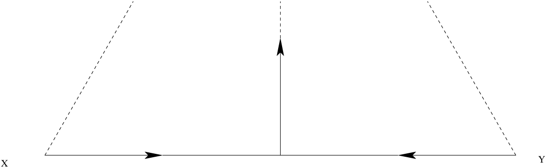
The signs of the fitnesses correspond to the arrows in each diagram. For example, $f(y;x)>0$ means that, on the edge of the simplex that reach $x$ and $y$ , there is an arrow starting from $x$ in the direction of $y$ . In other words, the unstable manifold of $(\bar{n}(x),0,0)$ contains (a part of) the edge of the simplex that reach $x$ to $y$ . Similarly, $f(z;x,y)>0$ means that $f(x;y)f(y;x)>0$ , i.e. that $\ LV(3,(x,y,z))$ has as fixed point $(\bar{n}_{1}(x,y),\bar{n}_{2}(x,y),0)$ , represented as the midpoint of the edge of the simplex linking $x$ and $y$ , and that this fixed point has an unstable manifold pointing in the direction of the interior of the simplex. The situation represented in Fig. 3.1 corresponds to this case, when $x$ and $y$ coexist.

In order to check if Assumption (B) holds, we only need to restrict to the equivalence classes in which two traits coexist (the resident traits, say $x$ and $y$ ), and the third (mutant) trait (say $z$ ) satisfy $f(z;x,y)>0$ . This situation corresponds to the cases where the carrying simplex has one side containing the pattern of Fig. 3.1. Among the 33 equivalence classes of [30], there are only 10 of them that satisfy this requirement, shown in Fig 3.2. We label them with the same numbers as in [30]. In Fig. 3.2, the figures obtained by exchanging $x$ and $y$ belong to the same equivalence class. An attracting fixed point of $LV(3,(x,y,z))$ is represented by a closed dot $\bullet$ , a repulsive fixed point by an empty dot $\circ$ , a saddle point by the intersection of its stable and unstable manifolds. When the interior fixed point (the non-trivial equilibrium) is not a saddle point, it can be either stable or unstable. Depending on cases, this equilibrium can also be surrounded by one or several stable or unstable cycles. In particular, the sign of the fitnesses is not sufficient to determine the precise asymptotic behavior of the system near the interior equilibrium. The undetermined type of these equilibria is represented in Fig. 3.2 by the symbol $\odot$ .

Since no pattern as in Fig. 2.4 occurs in diagrams 7 to 12 in Fig. 3.2, we see that Assumption (B1) is always satisfied except possibly in the cases of diagrams 26, 29, 31 and 33. It could be violated either if the interior equilibrium is surrounded by a stable cycle, or in diagram 26 in the case where the unstable manifold of the equilibrium $(\bar{n}_{1}(x,y),\bar{n}_{2}(x,y),0)$ (midpoint of the lower edge of the simplex) admits the equilibrium $(0,\bar{n}_{1}(y,z),\bar{n}_{2}(y,z))$ as limit point. Moreover, as before, all the steady states are hyperbolic if all the 2- and 3-dimensional fitnesses are nonzero.

Thus, if we define the set $C_{coex}$ as

C_{coex}:=\{(x,y,z)\in{\cal X}^{3}:LV(3,(x,y,z))\mbox{\ belongs to classes 26, 29, 31 or 33}\},

(3.6)

Assumption (B) will be satisfied for all $(x,y,z)\in{\cal X}^{3}\backslash C_{coex}$ as soon as Assumption (C2) is satisfied.

Remark in addition that, as checked from Fig. 3.2, if $x$ and $y$ coexist and $f(z;x,y)>0$ , then $(x,y,z)\in C_{coex}$ if and only if both of the following properties are satisfied

(P1): If $f(y;x,z)$ is well-defined, then $f(x;z)$ , $f(z;x)$ and $f(y;x,z)$ have all the same sign.
(P2): If $f(x;y,z)$ is well-defined, then $f(y;z)$ , $f(z;y)$ and $f(x;y,z)$ have all the same sign.

$\square$

Assumptions (C1) and (C2) will be summarized in Assumption (C).

Similarly as in Section 3.1, we define the killed PES $(Z_{t}^{(2)},t\geq 0)$ as a Markov pure jump process on ${\cal M}_{0}\cup\{\partial\}$ , with infinitesimal generator ${{\cal L}^{(2)}}$ . The latter is given by (2.12) for $d=1$ , and for $d=2$ and coexisting $x_{1},x_{2}$ , it is modified as follows. Let $\nu:=\sum_{i=1}^{2}\bar{n}_{i}(x_{1},x_{2})\delta_{x_{i}}$ , then

		$\displaystyle{{\cal L}^{(2)}}\varphi(\nu)=\int_{\mathbb{R}^{l}}\sum_{j=1}^{2}\Big(\varphi\Big(\sum_{i=1}^{2}n^{}_{i}(x_{1},x_{2},x_{j}+h)\delta_{x_{i}}+n^{}_{3}(x_{1},x_{2},x_{j}+h)\delta_{x_{j}+h}\Big)-\varphi(\nu)\Big)\times$
		$\displaystyle\quad p(x_{j})\lambda(x_{j})\bar{n}_{j}(x_{1},x_{2})\frac{[f(x_{j}+h;x_{1},x_{2})]_{+}}{\lambda(x_{j}+h)}\mathbf{1}_{\{(x_{1},x_{2},x_{j}+h)\not\in C_{coex}\}}m(x_{j},h)dh$
		$\displaystyle\quad+\int_{\mathbb{R}^{l}}\sum_{j=1}^{2}\big(\varphi(\partial)-\varphi(\nu)\big)p(x_{j})\lambda(x_{j})\bar{n}_{j}(x_{1},x_{2})\mathbf{1}_{\{(x_{1},x_{2},x_{j}+h)\in C_{coex}\}}m(x_{j},h)dh.$		(3.7)

This modification amounts to construct the killed PES as the PES, and send it to the cemetery state as soon as a mutant trait $x_{3}$ appears in a dimorphic population of traits $x_{1},x_{2}\in{\cal X}$ such that the Lotka Volterra dynamics associated with traits $x_{1},x_{2},x_{3}$ belongs to classes 26, 29, 31 or 33. Notice that the killed PES’s support has at most two traits at each time.

As in Section 3.1, we deduce the following results.

Proposition 3.6

Under Assumptions (A) and (C), the killed PES $(Z_{t}^{(2)},t\geq 0)$ is almost surely well-defined and belongs almost surely to ${\cal M}_{0}\cup\{\partial\}$ for all time.

Moreover this PES is the limiting process, on the mutation time scale, of the mutation-invasion process killed at the first triple-coexistence time.

Corollary 3.7

With the same assumption and notation as in Theorem 2.7, except that Assumption (B) is replaced by Assumption (C) and that $d\in\{1,2\}$ , let

\tilde{\tau}_{K}:=\inf\{t\geq 0:\mbox{Supp}(\nu_{t}^{K})=\{x,y,z\}\mbox{\ such that\ }(x,y,z)\in C_{coex}\}.

Then the process

\Big(\nu^{K}_{\frac{t}{Ku_{K}}}\mathbf{1}_{\{\frac{t}{Ku_{K}}\leq\tilde{\tau}_{K}\}}+\partial\ \mathbf{1}_{\{\frac{t}{Ku_{K}}>\tilde{\tau}_{K}\}},t\geq 0\Big)

converges as $K\rightarrow+\infty$ to the killed PES $(Z^{(2)}_{t},t\geq 0)$ with initial condition $Z^{(2)}_{0}=\sum_{i=1}^{d}\bar{n}_{i}(\mathbf{x})\delta_{x_{i}}$ .

Note that the killed PES obtained in this section is sufficient to study the phenomenon of evolutionary branching in Section 4 when ${\cal X}\subset\mathbb{R}$ .

4 Evolutionary branching and small jumps

We will assume, in all what follows, that the initial population is monomorphic, in the sense that at time $0$ , all individuals have the same trait.

We have seen in Section 3.1 that, as long as there is no coexistence of two traits in the population (Assumption (IIF)), the support of the PES is reduced to a single trait and the asymptotic dynamics of the population is given by the killed PES $Z^{(1)}$ with generator (3.1). In this section, our aim is to characterize the traits around which (IIF) fails and how evolutionary branching can occur in this case, as observed in Fig. 2.2(b). To do so, following a general idea of the biological literature [26, 8, 16, 15, 9, 14], a key assumption is that the mutation amplitude is small. In this situation, we will study the behavior of the PES on large time scales which will allow us to observe a global evolutionary dynamics.

In Subsection 4.1, we assume that (IIF) is always satisfied and we study the TSS with a small mutation step scaling $\varepsilon$ . We prove that on the longer time scale ${t\over\varepsilon^{2}}$ , the dynamics of the re-scaled TSS converges, when $\varepsilon$ tends to zero, to the solution of a (deterministic) ODE, called canonical equation of adaptive dynamics, or, more simply canonical equation. In Subsection 4.2, we come back to the general case. We show that (IIF) is satisfied on the time scale of the canonical equation and that evolutionary branching can only occur on a longer time scale. We are able to characterize the points, called “evolutionary singularities”, in the neighborhood of which evolutionary branching may occur. In Subsection 4.3, we state and prove our main result of this section, giving a criterion for evolutionary branching in the limit of small mutational jumps. We thus rigorously prove a criterion stated with a heuristic justification in [26].

Let us firstly introduce the following additional technical Assumptions (A’):

(A’1)

The trait space ${\cal X}$ is convex. It is often implicitly assumed for biological models with continuous trait space.

(A’2)

The distribution $m(x,h)dh$ has finite and bounded (in $x$ ) third-order moments.

(A’3)

The map $x\mapsto m(x,h)dh$ is Lipschitz continuous from ${\cal X}$ to the set of probability measures ${\cal P}(\mathbb{R}^{l})$ , for the Wasserstein metric

\rho(P_{1},P_{2})=\inf\Big\{\int_{{\mathbb{R}^{l}}\times{\mathbb{R}^{l}}}|x-y|\ R(dx,dy);R\in{\cal P}(\mathbb{R}^{l}\times\mathbb{R}^{l})\hbox{ with marginals }P_{1}\hbox{ and }P_{2}\Big\}.

(A’4)

The function

g(y;x)=p(x)\lambda(x)\bar{n}(x){f(y;x)\over\lambda(y)}

is continuous on ${\cal X}^{2}$ and of class ${\cal C}^{1}$ with respect to its first coordinate, where $f(\cdot;\cdot)$ is defined in (2.9). Since ${\cal X}$ is a compact set of ${\mathbb{R}}^{l}$ , there exists a constant $\gamma>0$ such that $\forall x,y\in{\cal X}$ , $\ [g(y;x)]_{+}\leq\gamma.$

Later in this section, we will also need Assumption (A”):

(A”): The functions $\lambda(x)$ and $\mu(x)$ are ${\cal C}^{3}$ on ${\cal X}$ and the function $\alpha(x,y)$ is ${\cal C}^{4}$ on ${\cal X}^{2}$ .

Note that (A”) implies (A’4).

Finally, let us introduce the parameter $\varepsilon\in(0,1]$ scaling the size of mutation. Since ${\cal X}$ is convex, $x+\varepsilon Y\in{\cal X}$ a.s. for all $x\in{\cal X}$ and $0\leq\varepsilon\leq 1$ , where $Y$ is distributed following $m(x,h)dh$ . Therefore, it is possible to define a PES in which mutational jumps are scaled by the parameter $\varepsilon$ , by replacing in its generator (2.12) $m(x_{j},h)dh$ by $m(x_{j},h)dh\circ H^{-1}_{\varepsilon}$ for all $j\in\{1,\ldots,d\}$ , where $H_{\varepsilon}(h)=\varepsilon h$ . Under Assumptions (A) and (B), we define this way a “rescaled PES” $(Z^{\varepsilon}_{t},t\geq 0)$ . If only Assumptions (A) and (C) are satisfied, we do similar changes in (3.7) to obtain a “rescaled killed PES” $(Z^{(2),\varepsilon}_{t},t\geq 0)$ . Finally, we do a time scaling of order $1/\varepsilon^{2}$ to obtain the rescaled PES

\tilde{Z}^{\varepsilon}_{t}=\begin{cases}Z^{\varepsilon}_{t/\varepsilon^{2}}&\mbox{if Assumptions~(A) and~(B) are satisfied}\\ Z^{(2),\varepsilon}_{t/\varepsilon^{2}}&\mbox{if only Assumptions~(A) and~(C) are satisfied.}\end{cases}

Since both $Z^{\varepsilon}_{t}$ and $Z^{(2),\varepsilon}_{t}$ agree as long as there is no triple coexistence, and since we will only be interested in the sequel to the cases where the PES is monomorphic or dimorphic, we will not need to distinguish between these two cases.

4.1 The TSS and the Canonical Equation of Adaptive Dynamics

Doing a similar time scaling as for $\tilde{Z}^{\varepsilon}$ , we can define for all $\varepsilon\in(0,1]$ , the $\varepsilon$ -rescaled TSS $(X^{\varepsilon}_{t},t\geq 0)$ by modifying the generator (3.2) as follows. For all ${\cal C}^{1}_{b}$ -valued function $\varphi$ ,

L^{\varepsilon}\varphi(x)=\frac{1}{\varepsilon^{2}}\int_{\mathbb{R}^{l}}(\varphi({x}+\varepsilon h)-\varphi({x}))[g(x+\varepsilon h;{x})]_{+}m(x,h)dh.

(4.1)

From a mathematical point of view, the multiplicative term $\varepsilon^{-2}$ takes into account that the integral term is of order $\varepsilon^{2}$ , because of $g(x;x)=0$ and Assumption (A’4).

Let us now state the convergence theorem of the rescaled TSS to the canonical equation of adaptive dynamics. Its proof is based on a standard uniqueness-compactness method.

Theorem 4.1

Assume (A) and (A’). Suppose also that the family of initial states $\{X^{\varepsilon}_{0}\}_{0<\varepsilon\leq 1}$ is bounded in $\mathbb{L}^{2}$ and converges in law to a random variable $X_{0}$ as $\varepsilon\rightarrow 0$ .

Then for each $T>0$ , the sequence $(X^{\varepsilon})$ converges when $\varepsilon\rightarrow 0$ , for the Skorohod topology of $\mathbb{D}([0,T],{\cal X})$ , to the process $({x}(t),t\leq T)$ with initial state $X_{0}$ and with deterministic sample paths, unique solution of the ordinary differential equation, known as canonical equation of adaptive dynamics.

\frac{dx}{dt}=\int_{\mathbb{R}^{l}}h[h\cdot\nabla_{1}g(x;{x})]_{+}\ m(x,h)dh.

(4.2)

Remark 4.2

In the case where $m(y,\cdot)$ is a symmetrical measure on $\mathbb{R}^{l}$ for all $y\in{\cal X}$ , Equation (4.2) gets the classical form, heuristically introduced in [8],

\frac{dx}{dt}=\frac{1}{2}K(x)\nabla_{1}g(x;{x}),

(4.3)

where $\ K(x)=\left(k_{ij}(x)\right)_{1\leq i,j\leq l}\$ is the covariance matrix of $m(x,h)dh$ .

Proof 9

(i) Uniqueness of the solution of Equation (4.2) with given initial condition.

Let us show that $\ a(x)=\int_{\mathbb{R}^{l}}h[h\cdot\nabla_{1}g(x;\mathbf{x})]_{+}\ m(x,h)dh$ is Lipschitz continuous on ${\cal X}$ . We have

\|a({x})-a({x}^{\prime})\|\leq\int_{\mathbb{R}^{l}}\|h\|\times\bigl|[h\cdot\nabla_{1}g(x;{x})]_{+}-[h\cdot\nabla_{1}g(x^{\prime};{x}^{\prime})]_{+}\bigr|\ m(x,h)dh\\ \quad+\left\|\int_{\mathbb{R}^{l}}h[h\cdot\nabla_{1}g(x^{\prime};{x}^{\prime})]_{+}(m(x,h)-m(x^{\prime},h))dh\right\|.

(4.4)

Because of $|[a]_{+}-[b]_{+}|\leq|a-b|$ , Assumptions (A’2) and (A’4), and that the support of all measures $m(x,h)dh$ is included in a bounded set, the first term of the right hand side of (4.4) is bounded by some constant times $\|{x}-{x}^{\prime}\|$ .

If we denote by $\xi$ the vector $\nabla_{1}g(x^{\prime};{x^{\prime}})$ and $\psi(h)=h[h\cdot\xi]_{+}$ , then

\|\psi(h)-\psi(h^{\prime})\|\leq\|(h-h^{\prime})[h\cdot\xi]_{+}\|+\|h^{\prime}([h\cdot\xi]_{+}-[h^{\prime}\cdot\xi]_{+})\|\leq 2\|\xi\|\ \|h-h^{\prime}\|\ (\|h\|+\|h^{\prime}\|).

Thus, using the dual form of the Kantorovich-Rubinstein metric (see Rachev [28]) and (A’3), one obtains that the second term of the right-hand side of (4.4) is also bounded by some constant times $\|x-x^{\prime}\|$ . Hence Cauchy-Lipschitz Theorem can be applied and $(\mathbf{x}(t),t\geq 0)$ is uniquely defined.

(ii) The processes $X^{\varepsilon},\,\varepsilon>0$ , with generator $L^{\varepsilon}$ can be constructed on the same probability space.

Recall the definition of $\gamma$ in Assumption (A’4).

Lemma 4.3

Assume (A) and (A’). Let $(\Omega,{\cal F},P)$ be a probability space and $N(dh,d\theta,ds)$ be a point Poisson measure on $\mathbb{R}^{l}\times[0,1]\times\mathbb{R}_{+}$ with intensity $\gamma\bar{m}(h)dhd\theta ds$ . Let $\varepsilon>0$ and denote by $N^{\varepsilon}$ the image measure of $N$ by the mapping $s\mapsto\varepsilon^{2}s$ . Let $X_{0}^{\varepsilon}$ be a ${\cal X}$ -valued random variable, independent of $N$ . Then the process $X^{\varepsilon}$ defined by

X^{\varepsilon}_{t}=X^{\varepsilon}_{0}+\int_{\mathbb{R}^{l}\times[0,1]\times[0,t]}(\varepsilon\,h)\ {\bf 1}_{\left\{\theta\leq{[g(X^{\varepsilon}_{s-}+\varepsilon h;X^{\varepsilon}_{s-})]_{+}\over\gamma}{m(X^{\varepsilon}_{s-},h)\over\bar{m}(h)}\right\}}N^{\varepsilon}(dh,d\theta,ds),

(4.5)

is a jump Markov process with generator $L^{\varepsilon}$ . Its law will be called $\mathbf{P}^{\varepsilon}_{X^{\varepsilon}_{0}}$ .

Indeed, using Itô’s formula, one observes that for a bounded function $\varphi$ on ${\cal X}$ ,

\varphi(X^{\varepsilon}_{t})-\varphi(X_{0}^{\varepsilon})\\ \hskip 14.22636pt-\int_{0}^{t}\int_{\mathbb{R}^{l}\times[0,1]}\left(\varphi(X^{\varepsilon}_{\varepsilon^{2}s}+\varepsilon h)-\varphi(X^{\varepsilon}_{\varepsilon^{2}s})\right){\bf 1}_{\{\varepsilon^{2}s\leq t\}}g(X^{\varepsilon}_{\varepsilon^{2}s}+\varepsilon h;X^{\varepsilon}_{\varepsilon^{2}s})m(X^{\varepsilon}_{\varepsilon^{2}s},h)dhd\theta ds

is a martingale, which implies the result.

(iii) Tightness of the sequence of laws $\{\mathbf{P}^{\varepsilon}_{X^{\varepsilon}_{0}}\}_{\varepsilon>0}$ .

We will use the Aldous criterion [1]. Let $\tau$ be a stopping time less than $T$ and $(\delta_{\varepsilon})$ positive numbers converging to $0$ when $\varepsilon\rightarrow 0$ . We remark that $|g(x+\varepsilon h;{x})|\leq\varepsilon C\|h\|$ , by an expansion of $g$ with respect to its first variable and the fact that $g(x;x)=0$ , and since $\nabla_{1}g$ is bounded by a constant $C$ . We have

\mathbf{E}(\|X^{\varepsilon}_{\tau+\delta_{\varepsilon}}-X^{\varepsilon}_{\tau}\|)=\mathbf{E}\left(\int^{\tau+\delta_{\varepsilon}}_{\tau}\int_{\mathbb{R}^{l}}\|\varepsilon h\|[g(X^{\varepsilon}_{s-}+\varepsilon h;X^{\varepsilon}_{s-})]_{+}\ m(X^{\varepsilon}_{s-},h)dh\frac{ds}{\varepsilon^{2}}\right)\leq CM_{2}\delta_{\varepsilon},

where $M_{2}=\int\|h\|^{2}\bar{m}(h)dh$ . Then, for any $\alpha>0$ ,

\mathbf{P}(\|X^{\varepsilon}_{\tau_{\epsilon}+\delta_{\varepsilon}}-X^{\varepsilon}_{\tau_{\varepsilon}}\|>\alpha)\leq\frac{nCM_{2}}{\alpha}\delta_{\varepsilon}\rightarrow 0\ \hbox{ when }\ \varepsilon\rightarrow 0.

This gives the first part of the Aldous criterion. For the second part, we have to prove the uniform tightness of the laws of $(\sup_{t\leq T}\|X^{\varepsilon}_{t}\|)_{\varepsilon>0}$ . We use Itô’s formula to write $(X^{\varepsilon}_{t})^{2}$ from (4.5), Schwarz’ and Doob’s inequalities and obtain that $\mathbf{E}(\sup_{t\leq T}\|X^{\varepsilon}_{t}\|^{2})\leq C_{T}(\mathbf{E}(\|X^{\varepsilon}_{0}\|^{2})+1)$ , where $C_{T}$ is a constant depending on time $T$ , on $M_{2}$ and on an upper-bound of $[g]_{+}$ . Since $(X_{0}^{\varepsilon})_{0<\varepsilon\leq 1}$ is bounded in $\mathbb{L}^{2}$ , the tightness of the laws of $(\sup_{t\leq T}\|X^{\varepsilon}_{t}\|)_{\varepsilon>0}\$ follows.

(iv) Convergence of the generators.

Let us now prove that

\forall\varphi\in{\cal C}^{2}_{b}({\cal X}),\ {1\over\varepsilon^{2}}L^{\varepsilon}\varphi\rightarrow L^{0}\varphi\mbox{\ uniformly on\ }{\cal X},

(4.6)

where $L^{\varepsilon}$ is defined in (3.2) and $L^{0}$ is defined by

L^{0}\varphi(\mathbf{x})=\int_{\mathbb{R}^{l}}(h\cdot\nabla\varphi({x}))[h\cdot\nabla_{1}g(x;{x})]_{+}\ m(x,h)dh,

where $\nabla\varphi({x})$ is the gradient vector of $\varphi({x})$ . We have,

\left|{1\over\varepsilon^{2}}L^{\varepsilon}\varphi({x})-L^{0}\varphi({x})\right|\leq\int_{\mathbb{R}^{l}}\![h\cdot\nabla_{1}g(x;{x})]_{+}\!\times\!\left|\frac{\varphi({x}+\varepsilon h)-\varphi({x})}{\varepsilon}-h\cdot\nabla\varphi({x})\right|m(x,h)dh\\ +\int_{\mathbb{R}^{l}}\left|\frac{\varphi({x}+\varepsilon h)-\varphi({x})}{\varepsilon}\right|\times\left|\left[\frac{g(x+\varepsilon h;{x})}{\varepsilon}\right]_{+}-[h\cdot\nabla_{1}g(x;x){x})]_{+}\right|m(x,h)dh.

(4.7)

Let us call $I_{1}$ and $I_{2}$ the quantities inside the integral in the first and the second term, respectively. Now, $\varphi$ is $\mathcal{C}^{1}$ , $g(x;{x})=0$ and by Assumption (A’), $g(x;y)$ is $\mathcal{C}^{1}$ with respect to the first variable $x$ . So, we can find $\theta_{1}$ , $\theta_{2}$ and $\theta_{3}$ in $[0,1]$ depending on ${x}$ and $h$ such that

	$\displaystyle I_{1}$	$\displaystyle=[h\cdot\nabla_{1}g(x;{x})]_{+}\times\|h\cdot\nabla\varphi({x}+\theta_{3}\varepsilon h)-h\cdot\nabla\varphi({x})\|;$
	$\displaystyle I_{2}$	$\displaystyle=\|h\cdot\nabla\varphi({x}+\theta_{1}\varepsilon h)\|\times\|[h\cdot\nabla_{1}g(x+\theta_{2}\varepsilon h;{x})]_{+}-[h\cdot\nabla_{1}g(x;{x})]_{+}\|.$

Since $\varphi$ is in $\mathcal{C}^{2}_{b}$ , and because of Assumption (A’), we can choose a number $C$ such that $\nabla\varphi$ and $\nabla_{1}g$ are both $C$ -Lipschitz and bounded by $C$ on ${\cal X}$ and ${\cal X}^{2}$ respectively. Then

	$\displaystyle I_{1}$	$\displaystyle\leq C\\|h\\|\times\\|h\\|C\\|\theta_{3}\varepsilon h\\|\leq\varepsilon C^{2}\\|h\\|^{3};$
	$\displaystyle I_{2}$	$\displaystyle\leq C\\|h\\|\times\|h\cdot\nabla_{1}g(x+\theta_{2}\varepsilon h,{x})-h\cdot\nabla_{1}g(x,{x})\|\leq\varepsilon C^{2}\\|h\\|^{3}.$

It remains to put these bounds in Equation (4.7) to obtain:

\left|{1\over\varepsilon^{2}}L^{\varepsilon}\varphi({x})-L^{0}\varphi({x})\right|\leq 2\varepsilon C^{2}\int_{\mathbb{R}^{l}}\|h\|^{3}m(x,h)dh.

We conclude using Assumption (A’2).

(v) Martingale problem for limiting distributions.

Finally, let us show that any accumulation point $\mathbf{P}$ of the family of laws $\{\mathbf{P}^{\varepsilon}_{X^{\varepsilon}_{0}}\}$ on $\mathbb{D}([0,T],{\cal X})$ is the law of the process ${X}$ solution to (4.2) with initial state $X_{0}$ . Fix such a $\mathbf{P}$ . Let us endow the space $\mathbb{D}([0,T],{\cal X})$ with the canonical filtration ${\cal G}_{t}$ , and for any $\varphi\in{\cal C}^{2}({\cal X})$ , let us define on this space the processes

	$\displaystyle M^{\varphi}_{t}(w)$	$\displaystyle=\varphi(w_{t})-\varphi(w_{0})-\int_{0}^{t}L^{0}\varphi(w_{s})ds$
	$\displaystyle M^{\varepsilon,\varphi}_{t}(w)$	$\displaystyle=\varphi(w_{t})-\varphi(w_{0})-\int_{0}^{t}{1\over\varepsilon^{2}}L^{\varepsilon}\varphi(w_{s})ds.$

We will show that $M^{\varphi}=0$ $\mathbf{P}$ -a.s. Fix $\varphi\in{\cal C}^{2}({\cal X})$ . It is standard, using Itô formula for jump processes, to show that, under $\mathbf{P}^{\varepsilon}_{X^{\varepsilon}_{0}}$ , $M^{\varepsilon,\varphi}$ is a square-integrable ${\cal G}_{t}$ -martingale and that

M^{\varepsilon,\varphi}_{t}(X^{\varepsilon})=\int_{\mathbb{R}^{l}\times[0,1]\times[0,t]}(\varphi(X^{\varepsilon}_{s}+\varepsilon h)-\varphi(X^{\varepsilon}_{s}))\\ \mathbf{1}_{\left\{\theta\leq\frac{[g(X^{\varepsilon}_{s-}+\varepsilon h,X^{\varepsilon}_{s-})]_{+}}{\gamma}\frac{m(X^{\varepsilon}_{s-},h)}{\bar{m}(h)}\right\}}\tilde{N}^{\varepsilon}\left(dh,d\theta,{ds}\right)

where $\tilde{N}^{\varepsilon}=N^{\varepsilon}-q^{\varepsilon}$ is the compensated Poisson measure associated with $N^{\varepsilon}$ , and $q^{\varepsilon}(dh,d\theta,ds)$ is the image measure of $\gamma\bar{m}(h)dhd\theta ds$ by $s\mapsto\varepsilon^{2}s$ . Thus, using computation similar to (4.1),

	$\displaystyle\mathbf{E}^{\varepsilon}(\langle M^{\varepsilon,\varphi}\rangle_{t})$	$\displaystyle=\frac{1}{\varepsilon^{2}}\mathbf{E}^{\varepsilon}\left(\int_{0}^{t}\int_{\mathbb{R}^{l}}(\varphi(X^{\varepsilon}_{s}+\varepsilon h)-\varphi(X^{\varepsilon}_{s}))^{2}[g(X^{\varepsilon}_{s}+\varepsilon h,X^{\varepsilon}_{s})]_{+}\ m(X^{\varepsilon}_{s},h)dhds\right)$
		$\displaystyle\leq CC^{\prime}M_{3}\,t\,\varepsilon,$		(4.8)

where $\mathbf{E}^{\varepsilon}$ denotes the expectation under $\mathbf{P}^{\varepsilon}_{X^{\varepsilon}_{0}}$ , $C^{\prime}$ is a bound for $\nabla\varphi$ , and $M_{3}$ a bound of the third-order moment of $m(y,h)dh$ . Using (4.8) and the fact that $M^{\varphi}_{t}(w)=M^{\varepsilon,\varphi}_{t}(w)+\int_{0}^{t}({1\over\varepsilon^{2}}L^{\varepsilon}\varphi(w_{s})-L^{0}\varphi(w_{s}))ds$ , it follows that

\mathbf{E^{\varepsilon}}(|M_{t}^{\varphi}|^{2})\leq 2t^{2}\|{1\over\varepsilon^{2}}\ L^{\varepsilon}\varphi-L^{0}\varphi\|^{2}_{\infty}+2C^{2}C^{\prime 2}M_{3}^{2}t^{2}\varepsilon^{2}

which converges to $0$ when $\varepsilon\rightarrow 0$ thanks to (4.6). Moreover by (4.5), we have that almost surely, $\ \sup_{t\leq T}\|X^{\varepsilon}_{t}-X^{\varepsilon}_{t-}\|\leq C^{\prime\prime}\varepsilon$ , which implies that each limit process $X$ with law $\mathbf{P}$ is almost surely continuous. Hence, for any $t\in[0,T]$ , the functional $\omega\mapsto\varphi(w_{t})-\varphi(w_{0})-\int_{0}^{t}L^{0}\varphi(w_{s})ds$ is continuous at $X$ for the weak topology and since $\mathbf{P}$ is the weak limit of an extracted sequence of $(\mathbf{P}^{\varepsilon}_{X^{\varepsilon}_{0}})$ , it follows that, under $\mathbf{P}$ , $M^{\varphi}(w)=0$ a.s, which concludes the proof. $\square$

4.2 PES and Evolutionary Singularities

Until the end of Section 4, we will assume for simplicity that the trait space is one-dimensional ( $l=1$ ), i.e. ${\cal X}\subset{\mathbb{R}}$ .

We have proved in the last subsection that, when $\varepsilon\to 0$ , the TSS is very close to the solution of the canonical equation (4.2) on any time interval $[0,T]$ . The equilibria of this equation are given by the points $x^{*}$ such that either $\partial_{1}g(x^{*};x^{*})=0$ , or $\int_{\mathbb{R}_{+}}m(x^{*},h)dh=0$ and $\partial_{1}g(x^{*};x^{*})>0$ , or $\int_{\mathbb{R}_{-}}m(x^{*},h)dh=0$ and $\partial_{1}g(x^{*};x^{*})<0$ . We will concentrate on the points such that $\partial_{1}g(x^{*};x^{*})=0$ , or equivalently, $\partial_{1}f(x^{*};x^{*})=0$ , since

\partial_{1}g(x;x)={1\over\lambda(x)}\partial_{1}f(x;x)p(x)\lambda(x)\bar{n}(x)=p(x)\bar{n}(x)\partial_{1}f(x;x).

Remark that, since $f(x;x)=0$ for all $x\in{\cal X}$ ,

		$\displaystyle\partial_{1}f(x;x)+\partial_{2}f(x;x)=0,\quad\forall x\in{\cal X}$		(4.9)
		$\displaystyle\partial_{11}f(x;x)+2\partial_{12}f(x;x)+\partial_{22}f(x;x)=0,\quad\forall x\in{\cal X}.$		(4.10)

Therefore, $\partial_{1}f(x^{*};x^{*})=\partial_{2}f(x^{*};x^{*})=0$ .

Definition 4.4

Points $x^{*}$ such that $\ \partial_{1}g(x^{*};x^{*})=0$ , or equivalently, $\partial_{1}f(x^{*};x^{*})=\partial_{2}f(x^{*};x^{*})=0$ are called evolutionary singularities (ES).

Lemma 4.5

Assume (A), (A’) and (A”).

(1): The solution $x(t)$ of (4.2) starting from a point that is not an ES cannot attain an ES in finite time.
(2): Assume that $x(0)$ is not an ES and let $I_{T}=\{x(t),t\in[0,T]\}$ . Then, for any sufficiently small $\eta>0$ , for any $x$ at a distance to $I_{T}$ smaller than $\eta$ and for any $y$ sufficiently close to $x$ , $x$ and $y$ satisfy (IIF) and $(y-x)f(y;x)$ has constant sign.

Proof 9 (1) Let $c$ be a constant such that $x\mapsto\int_{{\mathbb{R}}}h[h\cdot\partial_{1}g(x;x)]_{+}m(x,h)dh$ is $c$ -Lipschitz (the fact that this is a Lipschitz function is shown in the proof of Theorem 4.1). Then, for any ES $x^{*}$ ,

\Big|\frac{d}{dt}(x(t)-x^{*})^{2}\Big|\leq 2\ |\dot{x}(t)|\ |x(t)-x^{*}|\leq 2\ c\ (x(t)-x^{*})^{2}.

Thus, $|x(t)-x^{*}|\geq|x(0)-x^{*}|\exp(-ct)>0$ .

(2) Remark first that, from Point (1), $C=\inf_{x\in I_{T}}|\partial_{1}f(x(t);x(t))|>0.$ Therefore, for $\eta>0$ sufficiently small, $\{x\in{\cal X}:\mbox{dist}(x,I_{T})\leq\eta\}\subset\{x\in{\cal X}:|\partial_{1}f(x(t);x(t))|>C/2\}$ . Fix such an $\eta$ .

Let us now consider some point $x$ in ${\cal X}$ such that $\partial_{1}f(x;x)>C/2$ . Consider first $y$ in ${\cal X}$ such that $x<y$ . Using that $f(x;x)=0$ and (4.9), a second-order expansion of $f(y;x)$ at $(x,x)$ implies that $f(y;x)>C(y-x)/4$ provided that $|y-x|<{C\over 2C^{\prime}}$ , where $C^{\prime}>0$ is a constant uniformly upper-bounding the second-order derivatives of $f(\cdot;\cdot)$ on the compact set ${\cal X}^{2}$ . Under the same condition, $f(x;y)<C(x-y)/4$ . Therefore, $f(x;y)f(y;x)<0$ if $|y-x|$ is small enough and $(y-x)f(y;x)$ has constant sign. This reasoning gives the same conclusion if $y<x$ or $\partial_{1}f(x;x)<-C/2$ , giving the required result. $\square$

Now we come back to the rescaled PES $(\tilde{Z}^{\varepsilon}_{t},t\geq 0)$ defined in the beginning of this section and assume that its initial condition $\tilde{Z}^{\varepsilon}_{0}$ is monomorphic. We want to determine when evolutionary branching can occur in this process. This requires that (IIF) (ensuring non coexistence) fails. For $\varepsilon>0$ , we define the first coexistence time

\tau^{\varepsilon}=\inf\{t>0,\ f(\tilde{Z}^{\varepsilon}_{t},;\tilde{Z}^{\varepsilon}_{t-})>0\hbox{ and }f(\tilde{Z}^{\varepsilon}_{t-};\tilde{Z}^{\varepsilon}_{t})>0\},

and for any $\eta>0$ , the entrance time of the process in a $\eta$ -neighborhood of an ES $x^{*}$ ,

\theta^{\varepsilon}_{\eta}=\inf\{t\geq 0,\ \mbox{{Supp}}(\tilde{Z}^{\varepsilon}_{t})\cap(x^{*}-\eta,x^{*}+\eta)\not=\emptyset\}.

(4.11)

Theorem 4.6

Assume that (A), (A’), (A”) and (B) or (C) hold. Assume also that $\tilde{Z}_{0}^{\varepsilon}=\bar{n}(x)\delta_{x}$ where $x\in{\cal X}$ is not an evolutionary singularity. Then,

(i)

For any $T>0$ ,

\ \lim_{\varepsilon\rightarrow 0}\mathbb{P}(\tau^{\varepsilon}>T)=1.

Moreover, for all $\eta>0$ ,

\lim_{\varepsilon\rightarrow 0}\mathbb{P}(\forall t\in[0,T],\ \mbox{{Card}}(\mbox{{Supp}}(\tilde{Z}^{\varepsilon}_{t}))=1,\ \|\mbox{{Supp}}(\tilde{Z}^{\varepsilon}_{t})-x(t)\|\leq\eta)=1.

(ii)

For any $\eta>0$ , there exists $\varepsilon_{0}>0$ such that, for all $\varepsilon<\varepsilon_{0}$ ,

	$\displaystyle\mathbb{P}(\theta^{\varepsilon}_{\eta}<\tau^{\varepsilon})=1\quad\mbox{and}$
	$\displaystyle\mathbb{P}(\forall t\in[0,\theta^{\varepsilon}_{\eta}],\ \mbox{{Supp}}(\tilde{Z}^{\varepsilon}_{t})=\{Y^{\varepsilon}_{t}\}\ \mbox{with}\ t\mapsto Y^{\varepsilon}_{t}\ \mbox{monotonous on}\ [0,\theta^{\varepsilon}_{\eta}])=1.$		(4.12)

Proof 9 (i) Before the stopping time $\tau^{\varepsilon}$ , and since the initial condition is monomorphic, it is clear that the support of $\tilde{Z}^{\varepsilon}_{t}$ is a singleton whose dynamics is that of the rescaled TSS $(X^{\varepsilon}_{t},t\geq 0)$ . Because of Theorem 4.1, when $\varepsilon\to 0$ , the TSS is close to the canonical equation. In particular, for all $\eta>0$ , its values on the time interval $[0,T]$ belong to the set $\{x\in{\cal X}:\mbox{dist}(x,I_{T})\leq\eta\}$ with probability converging to 1. Moreover, since ${\cal X}$ is compact, $\mbox{Supp}(m(x,\cdot))\subset{\cal X}-x$ is included in the closed ball of $\mathbb{R}^{l}$ centered at 0 with diameter $2\mbox{diam}({\cal X})$ . Therefore, the distance between a mutant trait and the trait of its progenitor in the rescaled PES $\tilde{Z}^{\varepsilon}$ is a.s. less that $\varepsilon c$ , where $c$ is a constant. Hence, the result immediately follows from Lemma 4.5.

(ii) We also deduce from this lemma that for any $T>0$ such that $I_{T}\cap(x^{*}-3\eta/2,x^{*}+3\eta/2)=\emptyset$ , $\lim_{\varepsilon\rightarrow 0}\mathbb{P}(\theta^{\varepsilon}_{\eta}>T)=1$ . Moreover, the process $Y_{t}^{\varepsilon}$ in (4.12), which is exactly the TSS of the previous section, is almost surely monotonous before time $\theta^{\varepsilon}_{\eta}$ . $\square$

Remark 4.7

Theorem 4.6 implies that, when the initial population is monomorphic and away from evolutionary singularities, evolutionary branching can only occur in the neighborhood of an evolutionary singularity and on a longer time scale than $T/\varepsilon^{2}$ when $\varepsilon\rightarrow 0$ , for all $T>0$ .

The next result shows that we can restrict to ES that are not repulsive for the canonical equation.

Proposition 4.8

Under the assumptions of Theorem 4.6, coexistence of two traits can only occur in the neighborhood of evolutionary singularities $x^{*}\in{\cal X}$ which are not repulsive, i.e. which satisfy

\partial_{22}f(x^{*};x^{*})\geq\partial_{11}f(x^{*};x^{*}).

(4.13)

More precisely, for any neighborhood ${\cal U}$ of the set of evolutionary singularities satisfying (4.13), for all $\varepsilon$ small enough,

\mathbb{P}(\tau^{\varepsilon}<+\infty\mbox{\ and\ }\mbox{{Supp}}(Z^{\varepsilon}_{\tau^{\varepsilon}-})\not\in{\cal U})=0.

Proof 9 Let us remark that an ES such that

\partial_{11}f(x^{*};x^{*})+\partial_{12}f(x^{*};x^{*})>0.

(4.14)

is always a repulsive point for the canonical equation, in the sense that, for any solution $x(t)$ of the canonical equation starting sufficiently close from $x^{*}$ , the distance between $x(t)$ and $x^{*}$ is non-decreasing in the neighborhood of time 0. In other words, there exists a neighborhood ${\cal U}$ of $x^{*}$ such that no solution of the canonical equation starting out of ${\cal U}$ can enter ${\cal U}$ . To this end, we remark that (4.14) implies that there exists $\eta_{x^{*}}$ with

•

$\partial_{1}g(x;x)>0\$ if $\ x\in(x^{*},x^{*}+\eta_{x^{*}}]$ ,
•

$\partial_{1}g(x;x)<0\$ if $\ x\in[x^{*}-\eta_{x^{*}},x^{*})$ ,

and conclude in view of (4.2).

Observe that, by (4.10), (4.14) is equivalent to $\partial_{11}f(x^{*};x^{*})-\partial_{22}f(x^{*};x^{*})>0$ .

Let $S$ be the set of repulsive ES and define ${\cal V}=\cup_{x^{*}\in S}(x^{*}-\eta_{x^{*}},x^{*}-\eta_{x^{*}})$ . Fix ${\cal U}$ as in the statement of Proposition 4.8 and assume (without loss of generality) that ${\cal U}\cap{\cal V}=\emptyset$ and $x\not\in{\cal U}\cup{\cal V}$ . Let $[a,b]$ be any connected component of ${\cal X}\setminus({\cal U}\cup{\cal V})$ . Since $\partial_{1}f(y,y)\not=0$ for all $y\in[a,b]$ , reproducing the argument of the proof of Theorem 4.6 easily shows that coexistence never happens in a monomorphic population with trait in ${\cal X}\setminus({\cal U}\cup{\cal V})$ if $\varepsilon$ is sufficiently small. Similarly, for $\varepsilon$ sufficiently small, no mutant in ${\cal V}$ born from a monomorphic population with trait not belonging to ${\cal V}$ has a positive fitness. Therefore, the TSS cannot drive the population inside ${\cal V}$ starting from outside. Thus Proposition 4.8 is clear. $\square$

4.3 Evolutionary branching criterion

In this section we will prove a criterion of evolutionary branching. We need the following last assumption.

(A”’): For any $x$ in the interior of ${\cal X}$ , $\int_{\mathbb{R}_{-}}m(x,h)dh>0$ and $\int_{\mathbb{R}_{+}}m(x,h)dh>0$ .

4.3.1 Definition and main result

We first need to precisely define what we mean by evolutionary branching.

Definition 4.9

Let $x^{*}$ be an ES. For all $\eta>0$ , we call $\eta$ -branching the event

•

there exists $t_{1}>0$ such that the support of the PES at time $t_{1}$ is composed of a single point belonging to $[x^{*}-\eta,x^{*}+\eta]$
•

there exists $t_{2}>t_{1}$ such that the support of the PES at time $t_{2}$ is composed of exactly 2 points distant of more than $\eta/2$
•

between $t_{1}$ and $t_{2}$ , the support of the PES is always a subset of $[x^{*}-\eta,x^{*}+\eta]$ , and is always composed of at most 2 traits, and has increasing (in time) diameter.

We only consider binary evolutionary branching. We will actually prove that the simultaneous subdivision of a single branch into three branches (or more) is a.s. impossible. Note that this notion of evolutionary branching requires the coexistence of two traits, but also that these two traits diverge from one another.

Our main result is the following.

Theorem 4.10

Assume (A), (A’), (A”), (A”’) and either (B) or (C). Assume also that $Z^{\varepsilon}_{0}=\bar{n}(x)\delta_{x}$ and that the canonical equation with initial condition $x$ converges to an ES $x^{*}$ in the interior of ${\cal X}$ such that

		$\displaystyle\partial_{22}f(x^{};x^{})>\partial_{11}f(x^{};x^{})$		(4.15)
	and	$\displaystyle\partial_{22}f(x^{};x^{})+\partial_{11}f(x^{};x^{})\not=0.$		(4.16)

Then, for all sufficiently small $\eta$ , there exists $\varepsilon_{0}>0$ such that for all $\varepsilon<\varepsilon_{0}$ ,

(a)

if $\partial_{11}f(x^{*};x^{*})>0$ , $\mathbb{P}^{\varepsilon}(\eta\mbox{-branching})=1$ .

(b)

if $\partial_{11}f(x^{*};x^{*})<0$ , $\mathbb{P}^{\varepsilon}(\eta\mbox{-branching})=0$ . Moreover,

\mathbb{P}^{\varepsilon}\big(\forall t\geq\theta_{\eta}^{\varepsilon},\ \mbox{{Card}}(\mbox{{Supp}}(\tilde{Z}^{\varepsilon}_{t}))\leq 2\ \mbox{and}\ \mbox{{Supp}}(\tilde{Z}^{\varepsilon}_{t})\subset(x^{*}-\eta,x^{*}+\eta)\>\big)=1,

where $\theta_{\eta}^{\varepsilon}$ has been defined in (4.11).

This criterion appeared for the first time in [26] with an heuristic justification. We see that, locally around $x^{*}$ , one of the two following events can occur almost surely: either there is binary evolutionary branching and the two branches diverge monotonously, or there is no evolutionary branching, and the population stays forever inside any neighborhood of $x^{*}$ . Coexistence can occur in this case, but cannot drive the support of the population away from a small neighborhood of $x^{*}$ . We will actually prove that, in this case, as soon as there is coexistence of two traits in the population, the diameter of the support of the PES can only decrease until it reaches 0 (i.e. until the next time when the population becomes monomorphic).

We give in the following subsections a full proof of this result. In Section 4.3.3, we will prove regularity results on the 2- and 3-dimensional fitness functions and give their second order expansions in the neighborhood of evolutionary singularities. A first corollary of this result is given in Section 4.3.4 where, using the results of M.-L. Zeeman [30] and Fig. 3.2, we will show that no triple coexistence can occur in the neighborhood of evolutionary singularities. Finally, a case by case study of the zone of coexistence and of the signs of fitness functions in the neighborhood of an evolutionary singularity will allow us to conclude the proof in Section 4.3.5.

Before coming to the proof and in order to illustrate the difference between coexistence and evolutionary branching, we state a result that will be needed in the course of the proof of Theorem 4.10. Its proof will be given in Subsection 4.3.4. We recall that two traits $x$ and $y$ coexist if and only if $f(x;y)>0$ and $f(y;x)>0$ .

Proposition 4.11

Assume (A) and that $\lambda$ , $\mu$ and $\alpha$ are ${\cal C}^{2}$ . Let $x^{*}\in{\cal X}$ be any ES.

(a): If $\partial_{11}f(x^{*};x^{*})+\partial_{22}f(x^{*};x^{*})>0$ , then for all neighborhood ${\cal U}$ of $x^{*}$ , there exist $x,y\in{\cal U}$ that coexist.
(b): If $\partial_{11}f(x^{*};x^{*})+\partial_{22}f(x^{*};x^{*})<0$ , then there exists a neighborhood ${\cal U}$ of $x^{*}$ such that any $x,y\in{\cal U}$ do not coexist.

This shows that the criterion of evolutionary branching ( $\partial_{11}f(x^{*};x^{*})>0$ ) is different from the criterion of coexistence ( $\partial_{11}f(x^{*};x^{*})+\partial_{22}f(x^{*};x^{*})>0$ ). In particular, if one assumes as in Theorem 4.10 that $\partial_{22}f(x^{*};x^{*})>\partial_{11}f(x^{*};x^{*})$ , the evolutionary branching condition $\partial_{11}f(x^{*};x^{*})>0$ implies the coexistence criterion $\partial_{11}f(x^{*};x^{*})+\partial_{22}f(x^{*};x^{*})>0$ , as expected.

4.3.2 Example

Let us come back to the example introduced in Subsection 2.2.

The fitness function is

	$\displaystyle f(y;x)$	$\displaystyle=\lambda(y)-\alpha(y,x)\bar{n}(x)$
		$\displaystyle=\exp\Big(-{y^{2}\over 2\sigma^{2}_{b}}\Big)-\exp\Big(-{(x-y)^{2}\over 2\sigma^{2}_{\alpha}}\Big)\exp\Big(-{x^{2}\over 2\sigma^{2}_{b}}\Big).$

Computation gives

\partial_{1}f(x^{*};x^{*})=-{x^{*}\over\sigma^{2}_{b}}\exp\Big(-{(x^{*})^{2}\over 2\sigma^{2}_{b}}\Big)=0\Longleftrightarrow x^{*}=0.

Moreover, $\ \partial_{11}f(0;0)={1\over\sigma^{2}_{\alpha}}-{1\over\sigma^{2}_{b}}\$ and $\ \partial_{22}f(0;0)={1\over\sigma^{2}_{\alpha}}+{1\over\sigma^{2}_{b}}.$ Thus, the coexistence criterion of Proposition 4.11 (a) is always satisfied. We furthermore observe that (4.15) and (4.16) hold, and that

\partial_{11}f(0;0)>0\Longleftrightarrow\sigma_{\alpha}<\sigma_{b}.

Then if $\sigma_{\alpha}<\sigma_{b}$ , we have almost surely branching and when $\sigma_{\alpha}>\sigma_{b}$ , we have only coexistence. This is consistent with Fig. 2.2 (a) and (b).

4.3.3 Trait smoothness of fitnesses around evolutionary singularities

The problem of local expansion of fitness functions has been already studied in [10] for general models. In this section, we establish regularity and expansion results on our 2- and 3-dimensional fitness functions in the neighborhood of evolutionary singularities. To this aim, we need the following lemma.

Lemma 4.12

Let $h(x,y,z)$ be a ${\cal C}^{k}$ function for $k\geq 1$ defined on ${\cal X}^{3}$ such that $h(x,x,z)=0$ for all $x,z\in{\cal X}$ . Then, the function

(x,y,z)\mapsto\frac{h(x,y,z)}{x-y}

can be extended on $\{x=y\}$ as a ${\cal C}^{k-1}$ function $\hat{h}(x,y,z)$ on ${\cal X}^{3}$ by setting $\hat{h}(x,x,z)=\partial_{1}h(x,x,z)$ for all $x,z\in{\cal X}$ .

Proof 9 Taylor’s formula with integral remainder yields

\frac{h(x,y,z)}{x-y}=\int_{0}^{1}\partial_{1}h(y+(x-y)u,y,z)du

for all $x\not=y$ . The right-hand side also has a sense for $x=y$ and defines a ${\cal C}^{k-1}$ function on ${\cal X}^{3}$ . $\square$

Let $x^{*}\in{\cal X}$ be an ES as in the statement of Theorem 4.10. By Assumptions (A) and (A”), the 2-dimensional fitness function $f(y;x)$ defined in (2.9) is well-defined for all $x,y\in{\cal X}$ and is a ${\cal C}^{3}$ function. We extend the definition of the 3-dimensional fitness function

f(z;x,y)=r(z)-\alpha(z,x)\bar{n}_{1}(x,y)-\alpha(z,y)\bar{n}_{2}(x,y),

where $\bar{n}_{i}(x,y)$ , $i=1,2$ , are defined in (3.4) and (3.5) to all $x,y\in{\cal X}$ such that

\alpha(x,x)\alpha(y,y)-\alpha(x,y)\alpha(y,x)\neq 0.

We will also use the notation

a=\partial_{11}f(x^{*};x^{*})\quad\mbox{and}\quad c=\partial_{22}f(x^{*};x^{*}).

(4.17)

Note that, by (4.10),

\partial_{12}f(x^{*};x^{*})=-\frac{a+c}{2}.

(4.18)

Proposition 4.13

Under the assumptions of Theorem 4.10, the following properties hold.

(i)

For all $x,y\in{\cal X}$ in a neighborhood of $x^{*}$ ,

x\not=y\quad\Longrightarrow\quad\alpha(x,x)\alpha(y,y)\not=\alpha(x,y)\alpha(y,x).

This implies in particular that $\bar{\mathbf{n}}(x,y)$ and $f(\cdot;x,y)$ are well-defined for such $x,y$ .

(ii)

When $x,y\rightarrow x^{*}$ in such a way that $x\not=y$ , and for all $z\in{\cal X}$ ,

		$\displaystyle\bar{n}_{1}(x,y)+\bar{n}_{2}(x,y)\ \longrightarrow\ \bar{n}(x^{})=\frac{r(x^{})}{\alpha(x^{},x^{})};$		(4.19)
		$\displaystyle f(z;x,y)\ \longrightarrow\ f(z;x^{*}).$		(4.20)

(iii)

With the notation (4.17), as $x,y\rightarrow x^{*}$ ,

f(y;x)=\frac{1}{2}(x-y)\big(c(x-x^{*})-a(y-x^{*})\big)+o\big(|x-y|\,(|x-x^{*}|+|y-x^{*}|)\big).

(4.21)

(iv)

The function $f(z;x,y)$ can be extended as a ${\cal C}^{2}$ function on $\{(x,y,z):z\in{\cal X},x,y\in{\cal U}\}$ for some neighborhood ${\cal U}$ of $x^{*}$ in ${\cal X}$ . Still denoting by $f(z;x,y)$ the extended function, as $x,y\rightarrow x^{*}$ ,

f(z;x,y)=\frac{a}{2}(z-x)(z-y)+o\big(|z-x|\,|z-y|\big).

(4.22)

Proof 9 Let $D(x,y):=\alpha(x,x)\alpha(y,y)-\alpha(x,y)\alpha(y,x)$ . It follows from Lemma 4.12 that $D(x,y)/(x-y)$ can be extended on ${\cal X}^{2}$ as a ${\cal C}^{3}$ function, which has value

\partial_{1}\alpha(x,x)\alpha(x,x)+\partial_{2}\alpha(x,x)\alpha(x,x)-\partial_{1}\alpha(x,x)\alpha(x,x)-\alpha(x,x)\partial_{2}\alpha(x,x)=0

at the point $(x,x)$ . Therefore, Lemma 4.12 can be applied once more to prove that $D(x,y)/(x-y)^{2}$ can be extended as a ${\cal C}^{2}$ function $\hat{D}(x,y)$ on ${\cal X}^{2}$ . Hence, an elementary computation involving the second-order Taylor expansion of $D(x,y)$ yields that

D(x,y)=(x-y)^{2}\big(\alpha(x^{*},x^{*})\partial_{12}\alpha(x^{*},x^{*})-\partial_{1}\alpha(x^{*},x^{*})\partial_{2}\alpha(x^{*},x^{*})\big)+o(|x-y|^{2}).

Thus, Point (i) follows from the fact that $\alpha(x^{*},x^{*})\partial_{12}\alpha(x^{*},x^{*})\not=\partial_{1}\alpha(x^{*},x^{*})\partial_{2}\alpha(x^{*},x^{*})$ , which is a consequence of (4.16). Indeed, an elementary computation shows that

	$\displaystyle a=r^{\prime\prime}(x^{})-r(x^{})\frac{\partial_{11}\alpha(x^{},x^{})}{\alpha(x^{},x^{})}$
	$\displaystyle\begin{aligned} &\mbox{and}\quad c=-r^{\prime\prime}(x^{})+2r^{\prime}(x^{})\frac{\partial_{1}\alpha(x^{},x^{})}{\alpha(x^{},x^{})}\\ &+r(x^{})\frac{\alpha(x^{},x^{})\big(\partial_{11}\alpha(x^{},x^{})+2\partial_{12}\alpha(x^{},x^{})\big)-2\partial_{1}\alpha(x^{},x^{})\big(\partial_{1}\alpha(x^{},x^{})+\partial_{2}\alpha(x^{},x^{})\big)}{\alpha(x^{},x^{*})^{2}}.\end{aligned}$

Using the fact that

r^{\prime}(x^{*})=r(x^{*})\frac{\partial_{1}\alpha(x^{*},x^{*})}{\alpha(x^{*},x^{*})}

(4.23)

since $x^{*}$ is an ES, we have that

\alpha^{2}(x^{*},x^{*})(a+c)=2r(x^{*})\big(\alpha(x^{*},x^{*})\partial_{12}\alpha(x^{*},x^{*})-\partial_{1}\alpha(x^{*},x^{*})\partial_{2}\alpha(x^{*},x^{*})\big).

Hence,

\alpha(x^{*},x^{*})\partial_{12}\alpha(x^{*},x^{*})-\partial_{1}\alpha(x^{*},x^{*})\partial_{2}\alpha(x^{*},x^{*})\not=0\quad\Longleftrightarrow\quad a+c\not=0.

In particular, this implies that the function $\hat{D}(x,y)$ is non-zero in a neighborhood of $x^{*}$ .

For Point (ii), observe that

\bar{n}_{1}(x,y)+\bar{n}_{2}(x,y)=\frac{r(x)\frac{\alpha(y,y)-\alpha(y,x)}{x-y}+r(y)\frac{\alpha(x,x)-\alpha(x,y)}{x-y}}{(x-y)\hat{D}(x,y)}.

By the proof of Lemma 4.12, the numerator can be extended as a ${\cal C}^{3}$ function $h(x,y)$ by setting

h(x,y)=-r(x)\int_{0}^{1}\partial_{2}\alpha(y,y+(x-y)u)du+r(y)\int_{0}^{1}\partial_{2}\alpha(x,y+(x-y)u)du

for all $x,y\in{\cal X}$ . In particular, $h(x,x)=0$ for all $x\in{\cal X}$ . Therefore, Lemma 4.12 can be applied once more to prove that $\bar{n}_{1}(x,y)+\bar{n}_{2}(x,y)$ can be extended as a ${\cal C}^{2}$ function in the neighborhood of $x^{*}$ and that

\lim_{x,y\rightarrow x^{*},\,x\not=y}\bar{n}_{1}(x,y)+\bar{n}_{2}(x,y)=\frac{\frac{\partial h}{\partial x}(x^{*},x^{*})}{\hat{D}(x^{*},x^{*})}=\frac{r(x^{*})\partial_{12}\alpha(x^{*},x^{*})-r^{\prime}(x^{*})\partial_{2}\alpha(x^{*},x^{*})}{\alpha(x^{*},x^{*})\partial_{12}\alpha(x^{*},x^{*})-\partial_{1}\alpha(x^{*},x^{*})\partial_{2}\alpha(x^{*},x^{*})}.

Hence, (4.19) and then (4.20) follow from (4.23).

Point (iii) is obtained from the fact that $f(x;x)=0$ , from Lemma 4.12 and from the second-order Taylor expansion of $f(y;x)$ . In this computation, one must use the fact that $x^{*}$ is an ES and (4.18).

The fact that $f(z;x,y)$ is ${\cal C}^{2}$ in ${\cal U}\times{\cal U}\times{\cal X}$ can be proven exactly as the regularity of $\bar{n}_{1}(x,y)+\bar{n}_{2}(x,y)$ above, observing that

f(z;x,y)=r(z)-\frac{r(x)\frac{\alpha(z,x)\alpha(y,y)-\alpha(z,y)\alpha(y,x)}{x-y}+r(y)\frac{\alpha(z,y)\alpha(x,x)-\alpha(z,x)\alpha(x,y)}{x-y}}{(x-y)\hat{D}(x,y)}.

Therefore, using the fact that $f(x;x,y)=f(y;x,y)=0$ , Lemma 4.12 can be applied twice to prove that

f(z;x,y)=\frac{\gamma}{2}(z-x)(z-y)+o(|z-x|\,|z-y|)

for some constant $\gamma\in{\mathbb{R}}$ . The second-order Taylor expansion of $f(z;x,y)$ shows that $\gamma=\partial_{11}f(x^{*};x^{*},x^{*})$ . Now, because of (4.20), $\ \partial_{11}f(z;x^{*},x^{*})=\partial_{11}f(z;x^{*})$ for all $z\in{\cal X}$ . Hence $\gamma=a$ , which ends the proof of Point (iv). $\square$

Remark 4.14

Let us remark that, if $x^{*}$ is not an evolutionary singularity, Point (ii) of Proposition 4.13 need not to be true anymore, which may be surprising for the intuition and which has been a source of errors in some biological works.

Moreover, if $x^{*}$ is an ES but Assumption (4.16) ( $a+c\not=0$ ) is not true, Point (ii) of Proposition 4.13 may also fail. Indeed, in the case where $\alpha(x,x)\partial_{12}\alpha(x,x)\not=\partial_{1}\alpha(x,x)\partial_{2}\alpha(x,x)$ for $x\not=x^{*}$ ,

\bar{n}_{1}(x,x)+\bar{n}_{2}(x,x)=\frac{r(x)\partial_{12}\alpha(x,x)-r^{\prime}(x)\partial_{2}\alpha(x,x)}{\alpha(x,x)\partial_{12}\alpha(x,x)-\partial_{1}\alpha(x,x)\partial_{2}\alpha(x,x)}\\ =\frac{r(x^{*})\big(\partial_{112}\alpha(x^{*},x^{*})+\partial_{122}\alpha(x^{*},x^{*})\big)-r^{\prime}(x^{*})\partial_{22}\alpha(x^{*},x^{*})-r^{\prime\prime}(x^{*})\partial_{2}\alpha(x^{*},x^{*})+o(1)}{\alpha(x^{*},x^{*})\big(\partial_{112}\alpha(x^{*},x^{*})+\partial_{122}\alpha(x^{*},x^{*})\big)-\partial_{2}\alpha(x^{*},x^{*})\partial_{11}\alpha(x^{*},x^{*})-\partial_{1}\alpha(x^{*},x^{*})\partial_{22}\alpha(x^{*},x^{*})+o(1)}

as $x\rightarrow x^{*}$ . This expression involves $r^{\prime\prime}(x^{*})$ , whose value is not imposed by the assumptions. Therefore, changing the function $r$ in such a way that $r(x^{*})$ and $r^{\prime}(x^{*})$ are fixed but $r^{\prime\prime}(x^{*})$ changes also changes the value of $\lim_{x,y\rightarrow x^{*}}\bar{n}_{1}(x,y)+\bar{n}_{2}(x,y)$ .

4.3.4 On triple coexistence in the neighborhood of $x^{*}$

Points (iii) and (iv) of Proposition 4.13 allow one to determine the signs of the 2- and 3-dimensional fitnesses in a trimorphic population with traits $x,y,z$ close to $x^{*}$ . Combining this with the classification of Zeeman [30] (see Section 3.2 and Figure 3.2) gives the following corollary.

Corollary 4.15

For all ES $x^{*}$ satisfying the assumptions of Theorems 4.10 and such that $\partial_{11}f(x^{*};x^{*})\not=0$ , there exists a neighborhood ${\cal U}$ of of $x^{*}$ such that, for all distinct $x,y,z\in{\cal U}$ , $(x,y,z)\not\in C_{coex}$ , where $C_{coex}$ is defined in (3.6).

Proof 9 Let us assume for simplicity that $x^{*}=0$ . We shall distinguish between the cases $a>0$ and $a<0$ , and prove in each case that the fitnesses cannot have any of the sign configuration corresponding to the classes 26, 29, 31 and 33 in the neighborhood of $x^{*}$ . Since all these classes contain the pattern of Fig. 3.1, we can assume without loss of generality that $f(x;y)\geq 0$ , $f(y;x)\geq 0$ , $f(z;x,y)\geq 0$ and $x<y$ .

Consider first the case $a<0$ . It follows from Proposition 4.13 (iv) that the function $f(\cdot;\cdot,\cdot)$ has the shape of Fig. 4.1 (a) in the neighborhood of $x^{*}$ . In particular, this implies that $x<z<y$ , $f(z;x,y)>0$ , $f(x;y,z)<0$ and $f(y;x,z)<0$ as soon as $x,y,z$ are sufficiently close to $x^{*}$ . In view of Fig. 3.2, these conditions are incompatible with classes 31 and 33. Moreover, $\partial_{11}f(x;y)<0$ for all $x,y$ sufficiently close to $x^{*}$ . Therefore, by Lemma 4.12,

\frac{\partial}{\partial x}\Big(\frac{f(x;y)}{y-x}\Big)=-\int_{0}^{1}u\partial_{11}f(y+u(x-y);y)du

(4.24)

is positive for all $x,y$ sufficiently close to $x^{*}$ . Hence, since $x<z<y$ , we have $f(z;y)/(y-z)>f(x;y)/(y-x)\geq 0$ and thus $f(z;y)>0$ . Similarly, $f(z;x)>0$ . Together with $f(z;x,y)>0$ , these conditions are incompatible with classes 26 and 29. This ends the proof in the case where $a<0$ .

In the case where $a>0$ , by Proposition 4.13 (iv), $f(\cdot;\cdot,\cdot)$ has the shape of Fig. 4.1 (b) in the neighborhood of $x^{*}$ . Therefore, $z\not\in[x,y]$ . Assume for example that $\ z<x<y$ . By Proposition 4.13 (iv) again, $f(x;y,z)<0$ and $f(y;x,z)>0$ . These conditions are incompatible with class 33. Moreover, using the fact that $\partial_{11}f(x;y)>0$ for all $x,y$ sufficiently close to $x^{*}$ , it follows from the fact that (4.24) is negative that $f(z;y)/(y-z)>f(x;y)/(y-x)\geq 0$ and thus that $f(z;y)>0$ . Similarly, because of Assumption (4.15), $\partial_{22}f(x;y)>0$ for all $x,y$ sufficiently close to $x^{*}$ . Therefore, by Lemma 4.12,

\frac{\partial}{\partial x}\Big(\frac{f(y;x)}{y-x}\Big)=-\int_{0}^{1}u\partial_{22}f(y;y+u(x-y))du<0

for all $x,y$ sufficiently close to $x^{*}$ . Thus, $f(y;x)\geq 0$ implies that $f(y;z)>0$ . Together with the fact that $f(x;y,z)<0$ , these conditions are incompatible with classes 26, 29 and 31.

In the case where $\ x<y<z$ , the method above proves that $f(x;z)>0$ , $f(z;x)>0$ and $f(y;x,z)<0$ , which is again incompatible with classes 26, 29, 31 and 33. This ends the proof of Corollary 4.15. $\square$

4.3.5 Double coexistence region in the neighborhood of $x^{*}$

We prove here Proposition 4.11, that gives a criterion for the coexistence of two traits in the neighborhood of $x^{*}$ , and we end the proof of Theorem 4.10. The proof of Proposition 4.11 is based on the study of the region of double coexistence, defined as $\{(x,y)\in{\cal X}:f(x;y)>0\mbox{\ and\ }f(y;x)>0\}$ in the neighborhood of $x^{*}$ . The proof of Theorem 4.10 is based on a case-by-case study that extends the proof of Corollary 4.15.

Proof of Proposition 4.119 It follows from Proposition 4.13 (iii) that the set of $(x,y)\in{\cal X}$ such that $f(y;x)=0$ is composed of the line $\>\{y=x\}\>$ and of a set which is, because of the Implicit Function Theorem, a curve in the neighborhood of $x^{*}$ , containing $(x^{*},x^{*})$ and admitting as tangent at this point the line $\{a(y-x^{*})=c(x-x^{*})\}$ . Let us call $\gamma$ this curve. Since $a<c$ , the curves $\gamma$ and $\>\{y=x\}\>$ divide ${\cal X}^{2}$ in the neighborhood of $(x^{*},x^{*})$ into 4 regions. Moreover, because of (4.21), $f(y;x)$ changes sign when the point $(x,y)$ changes region by crossing either the line $\>\{y=x\}\>$ or the curve $\gamma$ .

It is elementary from a case-by-case study to check that coexistence can occur in the neighborhood of $x^{*}$ if $c>a>0$ , $a>c>0$ , $-a<c<0<a$ and $a<0<-a<c$ , and that coexistence cannot occur in the neighborhood of $x^{*}$ if $c<-a<0<a$ , $c<a<0$ , $a<c<0$ and $a<0<c<-a$ . The cases where coexistence is possible are represented in Fig. 4.2 in the case where $x^{*}=0$ . In these figures, the curve $\gamma$ is represented by its tangent line $\{a(y-x^{*})=c(x-x^{*})\}$ and the sign of $f(y;x)$ is represented by $+$ and $-$ signs depending on the position of $(x,y)$ with respect to $\gamma$ and $\>\{y=x\}$ . The sign of $f(x;y)$ is obtained by an axial symmetry of the figure with axis $\>\{y=x\}$ . We denote by $\gamma^{s}$ the symmetric of the curve $\gamma$ with respect to this axis. The region of coexistence is the one where $f(y;x)>0$ and $f(x;y)>0$ .

Note that the expansion of $f(y;x)$ of Proposition 4.13 (iii) does not make use of any assumption on $a$ and $c$ . Therefore, a similar study can be done to treat the degenerate cases. One easily obtains that coexistence is possible in the neighborhood of $(x^{*},x^{*})$ if $c=a>0$ , $c=0$ and $a>0$ or $a=0$ and $c>0$ . Similarly, coexistence cannot occur in the neighborhood of $(x^{*},x^{*})$ if $c=a<0$ , $c=0$ and $a<0$ or $a=0$ and $c<0$ . The case $c=-a$ is undetermined and depends on higher-order expansions of the fitness function. $\Box$

Proof of Theorem 4.10 (b): case $a<0$

It follows from Theorems 4.6 that for any fixed $\eta>0$ , for $\varepsilon$ small enough, the PES stays monomorphic until it reaches $(x^{*}-\eta,x^{*}+\eta)$ . Moreover, in view of the proof of Proposition 4.8, no mutant out of $(x^{*}-\eta,x^{*}+\eta)$ can invade the population as long as it is monomorphic with support inside this interval.

Now, by Proposition 4.11, when $a<0$ , coexistence may happen in the rescaled PES if $c>-a$ . In this case, at the first coexistence time $\tau^{\varepsilon}$ , the two traits $x$ and $y$ that coexist belong to $(x^{*}-\eta,x^{*}+\eta)$ and are distant of less than $\varepsilon\mbox{Diam}({\cal X})$ since $m(x,\cdot)$ has support in ${\cal X}-x$ .

Let us examine what happens when a mutant trait $z$ invades this population. Remind that we showed in the proof of Corollary 4.15 that, if $a<0$ , $x<y$ , $f(x;y)>0$ , $f(y;x)>0$ and $f(z;x,y)>0$ , then $f(x;y,z)<0$ , $f(y;x,z)<0$ , $f(z;y)>0$ and $f(z;x)>0$ . Examining Fig. 3.2, we see that these conditions are incompatible with all classes except classes 7 and 9. Therefore, once the mutant $z$ invades, the new state of the rescaled PES can be either $\bar{n}(z)\delta_{z}$ in the case of class 7, or either $\bar{n}_{1}(x,z)\delta_{x}+\bar{n}_{2}(x,z)\delta_{z}$ or $\bar{n}_{1}(y,z)\delta_{y}+\bar{n}_{2}(y,z)\delta_{z}$ in the case of class 9. In particular, we see that either the population becomes monomorphic again, or it stays dimorphic, but the distance between the two traits of the support of the PES has decreased. In addition, in both cases, the support of the new state of the PES is a subset of $(x^{*}-\eta,x^{*}+\eta)$ . Hence, $\eta$ -branching, as defined in Definition 4.9, cannot occur as soon as $\varepsilon<\eta/(2\mbox{Diam}({\cal X}))$ . This ends the proof of Theorem 4.10 (b). $\Box$

Proof of Theorem 4.10 (a): case $a>0$

By Proposition 4.11, when $a>0$ , under the assumptions of Theorem 4.10, we are in the situation of Fig. 4.2 (a), and hence coexistence is always possible in the neighborhood of $x^{*}$ . Fix $\eta>0$ . We are going to prove that, if $\eta$ is small enough, then for $\varepsilon$ small enough,

(i): the first time of coexistence $\tau^{\varepsilon}$ is a.s. finite and $\mbox{Supp}(Z^{\varepsilon}_{\tau^{\varepsilon}-})\subset(x^{*}-\eta,x^{*}+\eta)$ a.s.;
(ii): after time $\tau^{\varepsilon}$ , the distance between the two points of the support of the rescaled PES is non-descreasing and becomes a.s. bigger than $\eta/2$ in finite time, before exiting the interval $(x^{*}-\eta,x^{*}+\eta)$ .

These two points will clearly imply Theorem 4.10 (a).

For Point (i), observe first that, by Proposition 4.8, if $\tau^{\varepsilon}<+\infty$ , then $\mbox{Supp}(Z^{\varepsilon}_{\tau^{\varepsilon}-})\subset(x^{*}-\eta,x^{*}+\eta)$ . Thus we only have to prove that $\ \mathbb{P}(\tau^{\varepsilon}<\infty)=1$ .

In view of Fig. 4.2 (a), we observe that for a given jump size, the closer the support is from $x^{*}$ , the easier co-existence is. The proof is based on this fact, taking into account the additional difficulty that the jump rate is almost zero in that case.

Fix $\kappa>0$ . Let us define

\theta_{\kappa}=\inf\big\{t\geq 0:\ \mbox{Supp}(Z^{\varepsilon}_{t})\subset(x^{*}-\kappa\varepsilon,x^{*}+\kappa\varepsilon)\big\}.

From Assumptions (A’3) and (A”’), the functions

x\mapsto\int_{0}^{+\infty}h\>m(x,h)dh\quad\mbox{and}\quad x\mapsto\int_{-\infty}^{0}h\>m(x,h)dh

are continuous and there exists $\beta>0$ such that, for all $x\in[x^{*}-\eta,x^{*}+\eta]$ ,

\int_{0}^{+\infty}h\>m(x,h)dh>\beta>0\quad\mbox{and}\quad\int_{-\infty}^{0}h\>m(x,h)dh<-\beta<0.

(4.25)

It is thus elementary to check, using (4.21), that for any $x\in[x^{*}-\eta,x^{*}-\kappa\varepsilon]$ , resp. $x\in[x^{*}+\kappa\varepsilon,x^{*}+\eta]$ ,

		$\displaystyle\int_{\beta/2}^{+\infty}[g(x+\varepsilon h,x)]_{+}m(x,h)dh\geq C\varepsilon^{2}\beta\kappa>0\ ;$
	resp.	$\displaystyle\int^{-\beta/2}_{-\infty}[g(x+\varepsilon h,x)]_{+}m(x,h)dh\leq-C^{\prime}\varepsilon^{2}\beta\kappa<0.$

Assume that $\ \mathbb{P}(\tau^{\varepsilon}=\infty\ ;\ \theta_{\beta/2}=\infty)>0$ . Then, on this event, in view of (4.1), the previous inequalities show that there are infinitely many jumps in the TSS, with jump size bigger than $\varepsilon\beta/2$ . This yields a contradiction since the TSS is monotonous before $\tau^{\varepsilon}$ . Indeed, drawing a vertical line at some level $x$ in Fig. 4.2 (a) (for example the vertical dotted line), one can see that all the mutants invading the monomorphic population with trait $x$ either coexist with $x$ or are closer to $x^{*}$ than $x$ . On the other hand, it is clear from Fig. 4.2 that the first jump after time $\theta_{\beta/2}$ in the TSS with jump size bigger than $\varepsilon\beta/2$ (which almost surely happens) drives the TSS in the coexistence region. Therefore, $\ \mathbb{P}(\tau^{\varepsilon}=\infty\ ;\ \theta_{\beta/2}<\infty)=0$ and then $\ \mathbb{P}(\tau^{\varepsilon}=\infty)=0$ .

For Point (ii), assume that the rescaled PES is dimorphic at some time $t$ , with support $\{x,y\}$ , $x<y$ . Let us examine what happens when a mutant trait $z$ invades this population. Remind that we showed in the proof of Corollary 4.15 that, if $a>0$ and $x,y,z$ belong to $(x^{*}-\eta_{0},x^{*}+\eta_{0})$ for some $\eta_{0}>0$ and satisfy $x<y$ , $f(x;y)>0$ , $f(y;x)>0$ and $f(z;x,y)>0$ , then

•

either $z<x<y$ and $f(x;y,z)<0$ , $f(y;x,z)>0$ , $f(z;y)>0$ and $f(y;z)>0$ ,
•

or $x<y<z$ and $f(x;y,z)>0$ , $f(y;x,z)<0$ , $f(z;x)>0$ and $f(x;z)>0$ .

We can assume without loss of generality that $\eta<\eta_{0}$ . Examining Fig. 3.2, we see that both situations are only compatible with classes 9, 10, 11 and 12. Therefore, once the mutant $z$ invades, the new state of the rescaled PES is $\bar{n}_{1}(x,z)\delta_{x}+\bar{n}_{2}(x,z)\delta_{z}$ if $x<y<z$ or $\bar{n}_{1}(y,z)\delta_{y}+\bar{n}_{2}(y,z)\delta_{z}$ if $z<x<y$ . In both cases, we see that the distance between the two traits of the support of the PES can only increase until the stopping time $\theta^{\prime}$ where one of the points of the support leaves $(x^{*}-\eta,x^{*}+\eta)$ . In order to end the proof, it suffices to prove that, if $\eta$ is sufficiently small,

\theta^{\prime}<\infty\quad\mbox{\ a.s.}\quad\mbox{and}\quad\mbox{Diam}(\mbox{Supp}(\tilde{Z}^{\varepsilon}_{\theta^{\prime}}))>\eta/2.

The fact that $\theta^{\prime}<\infty$ a.s. can be proved using (4.25) in a similar way as for Point (i). The lower bound of the diameter of the PES immediately follows from the fact that

\tau^{\varepsilon}>\theta_{\kappa_{0}}\quad\mbox{\ a.s.,}\quad\mbox{where}\quad\kappa_{0}=\frac{2c\mbox{Diam({\cal X})}}{c-a}.

This inequality follows from the following argument: for any $x,y\in{\mathbb{R}}$ such that

|x-x^{*}|\geq\frac{2c|x-y|}{c-a},

(4.26)

it can be easily checked that

|y-x^{*}|\geq\frac{1}{2}\Big(1+\frac{a}{c}\Big)|x-x^{*}|\quad\hbox{and}\quad|y-x^{*}|\leq\Big(1+\frac{c-a}{2c}\Big)|x-x^{*}|.

Since $0<a<c$ , we have

\frac{1}{2}\Big(1+\frac{a}{c}\Big)>\frac{a}{c}\quad\mbox{and}\quad 1+\frac{c-a}{2c}<1+\frac{c-a}{a}=\frac{c}{a}.

Now, $\{(y-x^{*})=(c/a)(x-x^{*})\}$ is tangent to $\gamma$ at $(x^{*},x^{*})$ and $\{(y-x^{*})=(a/c)(x-x^{*})\}$ is tangent to $\gamma^{s}$ at $(x^{*},x^{*})$ . Therefore, in view of Fig. 4.2 (a), any $x,y\in{\mathbb{R}}$ satisfying (4.26) do not coexist together.

To conclude, it suffices to observe that, in the rescaled PES $\tilde{Z}$ , the distance between a mutant trait and the trait of its progenitor in the PES is always smaller than $\varepsilon\mbox{Diam}({\cal X})$ . Therefore, for any $x\in(x^{*}-\eta,x^{*}+\eta)$ such that $|x-x^{*}|\geq\varepsilon\kappa_{0}$ , any mutant trait $y$ born from $x$ do not coexist with $x$ . $\Box$

Appendix A Proof of Theorem 2.7

The proof of this result is very similar to the proof of [4, Thm.1]. We will not repeat all the details and we will restrict ourselves to the steps that must be modified. The general idea of the proof follows closely the heuristic argument of Section 2.4.1. Its skeleton is similar to the one in [4] for monomorphic populations.

For all $\varepsilon>0$ , $t>0$ , and $\Gamma\subset{\cal X}$ measurable, let

A_{\varepsilon,d}(t,\Gamma):=\Big\{\mbox{Supp}(\nu_{t/Ku_{K}})\subset\Gamma\mbox{\ has $d$ elements that coexist, say\ }x_{1},\ldots,x_{d},\\ \mbox{\ and\ }\forall 1\leq i\leq d,\ |\langle\nu_{t/Ku_{k}},\mathbf{1}_{\{x_{i}\}}\rangle-\bar{n}_{i}(\mathbf{x})|<\varepsilon\}.

To prove Theorem 2.7, we establish that for all $\varepsilon>0$ , $t>0$ and $\Gamma\subset{\cal X}$ measurable,

\lim_{K\rightarrow+\infty}\mathbb{P}(A_{\varepsilon,d}(t,\Gamma))=\mathbb{P}(\mbox{Supp}(Z_{t})\subset\Gamma\mbox{\ and has $d$ elements}).

(A.1)

where $(Z_{t},t\geq 0)$ is defined in Theorem 2.7. The first ingredient of the proof is the following proposition, which generalizes Theorem 3 (a) and (b) of [4].

Proposition A.1

Assume that, for any $K\geq 1$ , $\mbox{Supp}(\nu^{K}_{0})=\{x_{1},\ldots,x_{d}\}$ and $\langle\nu_{0}^{K},\mathbf{1}_{\{x_{i}\}}\rangle\in C$ a.s., where $C$ is a compact subset of ${\mathbb{R}}_{+}$ . Let $\phi(t,(n_{1},\ldots,n_{d}))$ denote the value at time $t$ of the solution of $LV(d,\mathbf{x})$ with initial condition $(n_{1},\ldots,n_{d})$ . Then, for all $T>0$ ,

\lim_{K\rightarrow+\infty}\sup_{1\leq i\leq d,\ t\in[0,T]}\Big|\langle\nu^{K}_{t},\mathbf{1}_{\{x_{i}\}}\rangle-\phi_{i}(t,(\langle\nu^{K}_{0},\mathbf{1}_{\{x_{1}\}}\rangle,\ldots,\langle\nu^{K}_{0},\mathbf{1}_{\{x_{d}\}}\rangle))\Big|=0\quad a.s.

(A.2)

This result is a direct corollary of Theorem 11.2.1 of [11], except for two small difficulties. The first one is that Theorem 11.2.1 of [11] assumes that the function $\mathbf{n}\mapsto F^{\mathbf{x}}(\mathbf{n})$ involved in the definition (2.4) of the Lotka Volterra system is uniformly Lipschitz on ${\mathbb{R}}_{+}^{d}$ , which is not the case. However, observe first that, if $n_{i}\leq M$ for some $M>0$ for all $i\in\{1,\ldots,d\}$ , then $\phi_{i}(t,(n_{1},\ldots,n_{d}))\leq M\vee(2\bar{\lambda}/\underline{\alpha})$ for all $t\geq 0$ . Indeed, if there is equality for some $t\geq 0$ and $i\in\{1,\ldots,d\}$ , then $\dot{\phi}_{i}(t,(n_{1},\ldots,n_{d}))<0$ . Therefore, the coefficients of the system $LV(d,\mathbf{x})$ are uniformly Lipschitz on the set of states that can be attained by the solution of the system starting from any initial conditions in a compact set. The second difficulty is that Theorem 11.2.1 of [11] only implies that (A.2) holds on the event where there is no mutation between $0$ and $T$ . In Lemma 2 (a) of [4], it is proved that for general initial condition $\nu^{K}_{0}$ , the probability of mutation on the time interval $[0,T]$ converges to 0, thus the conclusion follows.

The second ingredient is the following exponential deviation estimate on the so-called “problem of exit from an attracting domain” [13]. It generalizes Theorem 3 (c) of [4].

Proposition A.2

Let $x_{1},\ldots,x_{d}\in{\cal X}$ coexist. Then there exist constants $c,V>0$ such that, for any sufficently small $\varepsilon>0$ , if $(\langle\nu_{0}^{K},\mathbf{1}_{\{x_{i}\}}\rangle)_{1\leq i\leq d}$ belongs to the $(\varepsilon/2)$ -neighborhood of $\bar{\mathbf{n}}(\mathbf{x})$ , the time of exit of $(\langle\nu_{t}^{K},\mathbf{1}_{\{x_{i}\}}\rangle)_{1\leq i\leq d}$ from the $\varepsilon$ -neighborhhod of $\bar{\mathbf{n}}(\mathbf{x})$ is bigger than $e^{VK}\wedge\tau$ with probability converging to 1, where $\tau$ denotes the first mutation time. Moreover, the previous result also holds if, for all $i\in\{1,\ldots,d\}$ , the death rate of an individual with trait $x_{i}$

\mu(x_{i})+\sum_{j=1}^{d}\alpha(x_{i},x_{j})\langle\nu_{t}^{K},\mathbf{1}_{\{x_{j}\}}\rangle

(A.3)

is perturbed by an additional random process that is uniformly bounded by $c\varepsilon$ .

Such results are fairly standard and can be proved in a variety of ways. We let the proof to the reader. The first part of this proposition is used to prove that, when the first mutation occurs, the population densities have never left the $\varepsilon$ -neighborhood of $\bar{\mathbf{n}}(\mathbf{x})$ and the second is used to prove that, after the first mutation, as long as the mutant population is small, the resident population densities do not leave the $\varepsilon$ -neighborhood of $\bar{\mathbf{n}}(\mathbf{x})$ . In this case, the additional term in (A.3) is $\alpha(x_{i},y)\langle\nu_{t}^{K},\mathbf{1}_{\{y\}}\rangle$ , where $y$ is the mutant trait, which is smaller that $\bar{\alpha}\varepsilon$ if $\langle\nu_{t}^{K},\mathbf{1}_{\{y\}}\rangle\leq\varepsilon$ .

From these two results can be deduced the following lemma, which is the extension of Lemma 2 (b) and (c) of [4]. The proof is a simple copy of the argument in [4].

Lemma A.3

Let $\ \mbox{Supp}(\nu^{K}_{0})=\{x_{1},\ldots,x_{d}\}\$ that coexist and let $\tau$ denote the first mutation time. There exists $\varepsilon_{0}$ such that, if $(\langle\nu_{0}^{K},\mathbf{1}_{\{x_{i}\}}\rangle)_{1\leq i\leq d}$ belongs to the $\varepsilon_{0}$ -neighborhood of $\bar{\mathbf{n}}(\mathbf{x})$ , then, for any $\varepsilon<\varepsilon_{0}$ ,

	$\displaystyle\lim_{K\rightarrow+\infty}\mathbb{P}\Big(\tau>\log K,\ \sup_{1\leq i\leq d,\ t\in[\log K,\tau]}\|\langle\nu_{t}^{K},\mathbf{1}_{\{x_{i}\}}\rangle-\bar{n}_{i}(\mathbf{x})\|<\varepsilon\Big)=1,$
	$\displaystyle Ku_{K}\tau\ \overset{{\cal L}}{\underset{K\rightarrow\infty}{\Longrightarrow}}\ \mbox{{Exp}}\Big(\sum_{j=1}^{d}p(x_{j})\lambda(x_{j})\bar{n}_{j}(\mathbf{x})\Big)$
	$\displaystyle\mbox{and}\quad\lim_{K\rightarrow+\infty}\mathbb{P}(\mbox{at time $\tau$, the mutant is born from trait $x_{i}$})=\frac{p(x_{i})\lambda(x_{i})\bar{n}_{i}(\mathbf{x})}{\sum_{j=1}^{d}p(x_{j})\lambda(x_{j})\bar{n}_{j}(\mathbf{x})}$

for all $i\in\{1,\ldots,d\}$ , where $\>\overset{{\cal L}}{\Longrightarrow}\>$ denotes the convergence in law of real r.v. and $\mbox{{Exp}}(u)$ denotes the exponential law with parameter $u$ .

The fourth ingredient is the following lemma, which is an extension of Lemma 3 of [4].

Lemma A.4

Let $\mbox{Supp}(\nu^{K}_{0})=\{x_{1},\ldots,x_{d},y\}$ where $x_{1},\ldots,x_{d}$ coexist and $y$ is a mutant trait that satisfy Assumption (B). Let $\tau$ denote the first next mutation time, and define

	$\displaystyle\tau_{1}$	$\displaystyle=\inf\{t\geq 0:\forall i\in I(\mathbf{n}^{}),\ \|\langle\nu_{t}^{K},\mathbf{1}_{\{x_{i}\}}\rangle-n^{}_{i}\|<\varepsilon\mbox{\ and\ }\forall i\not\in I(\mathbf{n}^{*}),\ \langle\nu_{t}^{K},\mathbf{1}_{\{x_{i}\}}\rangle=0\}$
	$\displaystyle\tau_{2}$	$\displaystyle=\inf\{t\geq 0:\langle\nu_{t}^{K},\mathbf{1}_{\{y\}}\rangle=0\mbox{\ and\ }\forall i\in\{1,\ldots,d\},\ \|\langle\nu_{t}^{K},\mathbf{1}_{\{x_{i}\}}\rangle-\bar{n}_{i}(\mathbf{x})\|<\varepsilon\}.$

Assume that $\langle\nu_{0}^{K},\mathbf{1}_{\{y\}}\rangle=1/K$ (a single initial mutant). Then, there exists $\varepsilon_{0}$ such that for all $\varepsilon<\varepsilon_{0}$ , if $(\langle\nu_{0}^{K},\mathbf{1}_{\{x_{i}\}}\rangle)_{1\leq i\leq d}$ belongs to the $\varepsilon$ -neighborhood of $\bar{\mathbf{n}}(\mathbf{x})$ ,

	$\displaystyle\lim_{K\rightarrow+\infty}\mathbb{P}(\tau_{1}<\tau_{2})=\frac{[f(y;\mathbf{x})]_{+}}{\lambda(y)},\quad\lim_{K\rightarrow+\infty}\mathbb{P}(\tau_{2}<\tau_{1})=1-\frac{[f(y;\mathbf{x})]_{+}}{\lambda(y)}$
	$\displaystyle\mbox{and}\quad\forall\eta>0,\quad\lim_{K\rightarrow+\infty}\mathbb{P}\left(\tau_{1}\wedge\tau_{2}<\frac{\eta}{Ku_{K}}\wedge\tau\right)=1.$

The proof of this lemma is similar to the proof of Lemma 3 in [4]. The main steps are the following. Assume first that $\varepsilon<1/2$ . We introduce the following stopping times:

	$\displaystyle R_{\varepsilon}^{K}$	$\displaystyle=\inf\{t\geq 0:\exists i\in\{1,\ldots,d\},\ \|\langle\nu_{t}^{K},\mathbf{1}_{\{x_{i}\}}\rangle-\bar{n}_{i}(\mathbf{x})\|\geq\varepsilon\}$
	$\displaystyle S_{\varepsilon}^{K}$	$\displaystyle=\inf\{t\geq 0:\langle\nu_{t}^{K},\mathbf{1}_{\{y\}}\rangle\geq\varepsilon\}$
	$\displaystyle S_{0}^{K}$	$\displaystyle=\inf\{t\geq 0:\langle\nu_{t}^{K},\mathbf{1}_{\{y\}}\rangle=0\}.$

$R^{K}_{\varepsilon}$ is the time of drift of the resident population away from its equilibrium, $S_{\varepsilon}^{K}$ is the time of invasion of the mutant trait (time $t_{1}$ in Fig. 2.3) and $S_{0}^{K}$ is the time of extinction of the mutant trait. By the second part of Proposition A.2, it can be proven exactly as in [4] that there exists $\rho,V>0$ and $c<1$ such that, for $K$ large enough,

\mathbb{P}\Big(\frac{\rho}{Ku_{K}}<\tau\Big)\geq 1-\varepsilon\quad\mbox{and}\quad\mathbb{P}(S^{K}_{\varepsilon}\wedge\tau\wedge e^{KV}<R^{K}_{\varepsilon/c})\geq 1-\varepsilon.

Then, on $[0,\tau\wedge S_{\varepsilon}^{K}\wedge R^{K}_{\varepsilon/c}]$ , by computing lower and upper bounds on the death rate of a mutant individual, it can be easily checked that, for $K$ large enough, almost surely,

\frac{Z^{1,\varepsilon}_{t}}{K}\leq\langle\nu_{t}^{K},\mathbf{1}_{\{y\}}\rangle\leq\frac{Z^{-1,\varepsilon}_{t}}{K}

where, for $i=1$ or $-1$ , $Z^{i,\varepsilon}$ is a continuous-time branching process such that $Z^{i,\varepsilon}_{0}=1$ and with birth rate $(1-i\varepsilon)\lambda(y)$ and death rate

\mu(y)+\sum_{j=1}^{d}\alpha(y,x_{i})\bar{n}_{i}(\mathbf{x})+i(d+1)\bar{\alpha}\frac{\varepsilon}{c}.

Next, we use the results of Theorem 4 of [4] on branching processes in order to control the probability that $Z^{i,\varepsilon}/K$ exceeds $\varepsilon$ before it reaches 0, and to upper bound the time at which one of these events happens. As in [4], we obtain that there exists $C>0$ such that, for all $\eta>0$ , $\varepsilon>0$ sufficiently small and $K$ large enough,

	$\displaystyle\mathbb{P}\Big(\tau_{2}<\tau\wedge\frac{\eta}{Ku_{K}}\wedge S^{K}_{\varepsilon}\wedge R^{K}_{\varepsilon/c}\Big)$	$\displaystyle\geq 1-\frac{[f(y;\mathbf{x})]_{+}}{\lambda(y)}-C\varepsilon$		(A.4)
	$\displaystyle\mathbb{P}\Big(S_{\varepsilon}^{K}<\tau\wedge\frac{\eta}{Ku_{K}}\wedge S^{K}_{0}\wedge R^{K}_{\varepsilon/c}\Big)$	$\displaystyle\geq\frac{[f(y;\mathbf{x})]_{+}}{\lambda(y)}-C\varepsilon.$

On the event $\{S_{\varepsilon}^{K}<\tau\wedge S^{K}_{0}\wedge R^{K}_{\varepsilon/c}\}$ , we introduce for $\varepsilon^{\prime}>0$ the stopping times

	$\displaystyle T^{K}_{\varepsilon}$	$\displaystyle=\inf\{t\geq S_{\varepsilon}^{K}:\forall i\in\{1,\ldots,d\},\ \|\langle\nu_{t}^{K},\mathbf{1}_{\{x_{i}\}}\rangle-n^{}_{i}\|<\varepsilon^{2}\mbox{\ and\ }\|\langle\nu_{t}^{K},\mathbf{1}_{\{y\}}\rangle-n^{}_{d+1}\|<\varepsilon^{2}\},$
	$\displaystyle U^{K}_{\varepsilon,\varepsilon^{\prime}}$	$\displaystyle=\inf\{t\geq T^{K}_{\varepsilon}:\exists i\in I(\mathbf{n}^{}),\ \|\langle\nu_{t}^{K},\mathbf{1}_{\{x_{i}\}}\rangle-n^{}_{i}\|\geq\varepsilon^{\prime}\}$
	$\displaystyle V^{K}_{\varepsilon}$	$\displaystyle=\inf\{t\geq T^{K}_{\varepsilon}:\exists i\not\in I(\mathbf{n}^{*}),\ \langle\nu_{t}^{K},\mathbf{1}_{\{x_{i}\}}\rangle\geq\varepsilon\}.$

We next use the Markov property at time $S_{\varepsilon}^{K}$ and apply Proposition A.1 as in [4] to obtain that there exists $C^{\prime}>C$ such that, for $K$ large enough,

\mathbb{P}\Big(S_{\varepsilon}^{K}<T^{K}_{\varepsilon}<\tau\wedge\frac{\eta}{Ku_{K}}\Big)\geq\frac{[f(y;\mathbf{x})]_{+}}{\lambda(y)}-C^{\prime}\varepsilon.

Next, we can use again Proposition A.2 to prove that there exists $V^{\prime}>0$ , $C^{\prime\prime}>C^{\prime}$ and $c^{\prime}<1$ such that

\mathbb{P}\big(S_{\varepsilon}^{K}<T^{K}_{\varepsilon}<V_{\varepsilon}^{K}\wedge\tau\wedge e^{KV^{\prime}}<U^{K}_{\varepsilon,\varepsilon/c^{\prime}}\big)\geq\frac{[f(y;\mathbf{x})]_{+}}{\lambda(y)}-C^{\prime\prime}\varepsilon.

In a last step, we can as before prove that, for all $t\in[T_{\varepsilon}^{K},U^{K}_{\varepsilon,\varepsilon/c^{\prime}}\wedge V^{K}_{\varepsilon}]$ and for all $i\not\in I(\mathbf{n}^{*})$ ,

\langle\nu^{K}_{t},\mathbf{1}_{\{x_{i}\}}\rangle\leq\frac{\tilde{Z}^{i,\varepsilon}_{t}}{K},

where $\tilde{Z}^{i,\varepsilon}$ is a continuous-time branching process such that $\tilde{Z}^{i,\varepsilon}_{T_{\varepsilon}^{K}}=\lceil\varepsilon^{2}K\rceil$ and with birth rate $\lambda(x_{i})$ and death rate

\mu(x_{i})+\sum_{j\in I(\mathbf{n}^{*})}\alpha(x_{i},x_{j})n^{*}_{j}-\mbox{Card}(I(\mathbf{n}^{*}))\bar{\alpha}\frac{\varepsilon}{c^{\prime}}.

Since, by Assumption (B2), $f(x_{i};\mathbf{x}^{*})<0$ , this branching process is sub-critical if $\varepsilon$ is small enough. Hence, with arguments similar to the ones in [4] (especially the results of Theorem 4), we can prove that there exist $C^{\prime\prime\prime}>0$ such that, for all $\eta>0$ , $\varepsilon>0$ sufficiently small and $K$ large enough,

\mathbb{P}\Big(S^{K}_{\varepsilon}<\tau_{1}<\tau\wedge\frac{\eta}{Ku_{K}}\wedge U^{K}_{\varepsilon,\varepsilon/c^{\prime}}\Big)\geq\frac{[f(y;\mathbf{x})]_{+}}{\lambda(y)}-C^{\prime\prime\prime}\varepsilon.

Combining this with (A.4), we obtain Lemma A.4 by letting $\varepsilon$ go to 0.

Finally, (A.1) is deduced from these lemmas exactly as in [4] and similarly, the proof of Theorem 2.7 from (A.1). $\Box$

Acknowledgements9 We thank Michel Benaïm and Salome Martinez who brought to our attention the reference [30] and Michel Benaïm for helpful suggestions concerning Lotka-Volterra systems.

References

[1] D. Aldous. Stopping times and tightness. Ann. Probab., 6(2):335–340, 1978.
[2] G. Barles and B. Perthame. Concentrations and constrained Hamilton-Jacobi equations arising in adaptive dynamics. Preprint, 2006.
[3] A. Bovier and N. Champagnat. Time scales in adaptive dynamics: directional selection, fast and slow branching. In prep.
[4] N. Champagnat. A microscopic interpretation for adaptive dynamics trait substitution sequence models. Stoch. Process. Appl., 116(8):1127–1160, 2006.
[5] N. Champagnat, R. Ferrière, and S. Méléard. Unifying evolutionary dynamics: From individual stochastic processes to macroscopic evolution. Theor. Pop. Biol., 69:297–321, 2006.
[6] N. Champagnat, R. Ferrière, and S. Méléard. Individual-based probabilistic models of adaptive evolution and various scaling approximations. In Seminar on Stochastic Analysis, Random Fields and Applications V, volume 59 of Progr. Probab., pages 75–113. Birkhäuser, Basel, 2008.
[7] U. Dieckmann and M. Doebeli. On the origin of species by sympatric speciation. Nature, 400:354–357, 1999.
[8] U. Dieckmann and R. Law. The dynamical theory of coevolution: a derivation from stochastic ecological processes. J. Math. Biol., 34(5-6):579–612, 1996.
[9] O. Diekmann, P.-E. Jabin, S. Mischler, and B. Perthame. The dynamics of adaptation: An illuminating example and a Hamilton-Jacobi approach. Theor. Pop. Biol., 67:257–271, 2005.
[10] M. Durinx, J. A. J. Metz, and G. Meszéna. Adaptive dynamics for physiologically structured population models. J. Math. Biol., 56(5):673–742, 2008.
[11] S. N. Ethier and T. G. Kurtz. Markov processes. Characterization and convergence. Wiley Series in Probability and Mathematical Statistics: Probability and Mathematical Statistics. John Wiley & Sons Inc., New York, 1986.
[12] N. Fournier and S. Méléard. A microscopic probabilistic description of a locally regulated population and macroscopic approximations. Ann. Appl. Probab., 14(4):1880–1919, 2004.
[13] M. I. Freidlin and A. D. Wentzell. Random perturbations of dynamical systems, volume 260 of Grundlehren der Mathematischen Wissenschaften [Fundamental Principles of Mathematical Sciences]. Springer-Verlag, New York, 1984. Translated from the Russian by Joseph Szücs.
[14] S. A. H. Geritz. Resident-invader dynamics and the coexistence of similar strategies. J. Math. Biol., 50(1):67–82, 2005.
[15] S. A. H. Geritz, M. Gyllenberg, F. J. A. Jacobs, and K. Parvinen. Invasion dynamics and attractor inheritance. J. Math. Biol., 44(6):548–560, 2002.
[16] S. A. H. Geritz, J. A. J. Metz, E. Kisdi, and G. Meszena. The dynamics of adaptation and evolutionary branching. Phys. Rev. Lett., 78:2024–2027, 1997.
[17] S. A. H. Geritz, E. van der Meijden, and J. A. J. Metz. Evolutionary dynamics of seed size and seedling competitive ability. Theor. Pop. Biol., 55:324–343, 1999.
[18] J. Guckenheimer and P. Holmes. Nonlinear oscillations, dynamical systems, and bifurcations of vector fields, volume 42 of Applied Mathematical Sciences. Springer-Verlag, New York, 1983.
[19] M. W. Hirsch. Systems of differential equations which are competitive or cooperative. III. Competing species. Nonlinearity, 1(1):51–71, 1988.
[20] M. W. Hirsch. On existence and uniqueness of the carrying simplex for competitive dynamical systems. Journal of Biological Dynamics, 2(2):169–179, 2008.
[21] J. Hofbauer and K. Sigmund. Adaptive dynamics and evolutionary stability. Appl. Math. Lett., 3(4):75–79, 1990.
[22] J. Istas. Mathematical modeling for the life sciences. Universitext. Springer-Verlag, Berlin, 2005.
[23] N. L. Kaplan, R. R. Hudson, and C. H. Langley. The hitch-hiking effect revisited. Genetics, 123:887–899, 1989.
[24] E. Kisdi. Evolutionary branching under asymmetric competition. J. Theor. Biol., 197:149–162, 1999.
[25] P. Marrow, R. Law, and C. Cannings. The coevolution of predator-prey interactions: ESSs and red queen dynamics. Proc. R. Soc. Lond. B, 250:133–141, 1992.
[26] J. A. J. Metz, S. A. H. Geritz, G. Meszéna, F. J. A. Jacobs, and J. S. van Heerwaarden. Adaptive dynamics, a geometrical study of the consequences of nearly faithful reproduction. In Stochastic and spatial structures of dynamical systems (Amsterdam, 1995), Konink. Nederl. Akad. Wetensch. Verh. Afd. Natuurk. Eerste Reeks, 45, pages 183–231. North-Holland, Amsterdam, 1996.
[27] J. A. J. Metz, R. M. Nisbet, and S. A. H. Geritz. How should we define ’fitness’ for general ecological scenarios? Trends Ecol. Evol., 7:198–202, 1992.
[28] S. T. Rachev. Probability metrics and the stability of stochastic models. Wiley Series in Probability and Mathematical Statistics: Applied Probability and Statistics. John Wiley & Sons Ltd., Chichester, 1991.
[29] J. A. Roughgarden. Theory of population genetics and evolutionary ecology: an introduction. Macmillan, New York, 1979.
[30] M. L. Zeeman. Hopf bifurcations in competitive three-dimensional Lotka-Volterra systems. Dynam. Stability Systems, 8(3):189–217, 1993.