Systematic Perturbation Theory for Dynamical Coarse-Graining

Gernot Schaller^∗, Philipp Zedler, and Tobias Brandes Affiliation: Institut für Theoretische Physik, Technische Universität Berlin, Hardenbergstr. 36, 10623 Berlin, Germany

Abstract

We demonstrate how the dynamical coarse-graining approach can be systematically extended to higher orders in the coupling between system and reservoir. Up to second order in the coupling constant we explicitly show that dynamical coarse-graining unconditionally preserves positivity of the density matrix – even for bath density matrices that are not in equilibrium and also for time-dependent system Hamiltonians. By construction, the approach correctly captures the short-time dynamics, i.e., it is suitable to analyze non-Markovian effects. We compare the dynamics with the exact solution for highly non-Markovian systems and find a remarkable quality of the coarse-graining approach. The extension to higher orders is straightforward but rather tedious. The approach is especially useful for bath correlation functions of simple structure and for small system dimensions.

Keywords:

Lindblad form, positivity, non-Markovian master equation

pacs

03.65.Yz, 31.15.Md, 03.67.-a

I Introduction

The insight that quantum computers may solve certain problems such as number factoring [1] and database search [2] more efficiently than conventional computers has given rise to the field of quantum information (for an overview see e.g. [3]). The conventional paradigm of quantum computation relies on unitary operations that act on low-dimensional subspaces of the $2^{n}$ -dimensional Hilbertspace of $n$ two-level systems – conventionally called qubits. Unfortunately, the dynamics of open quantum systems is not always unitary [4], such that the impact of decoherence has to be taken into account. This problem also affects alternative schemes such as one-way [5, 6], holonomic [7] or adiabatic [8] quantum computation. Beyond this, the study of decoherence effects is of general interest in the control of quantum systems.

Often, the dynamics of open quantum systems is analyzed within the Born-Markov approximation scheme [4, 9]. An important criticism raised against this scheme is that it does not generally preserve positivity of the reduced density matrix [12, 13, 14, 15], which however is necessary for its probability interpretation [16]. In addition, the Born-Markov master equation cannot be expected to yield good results for short times, which may in the context of quantum computation for example lead to false error estimates on required gate operation times etc [10, 11].

A possible resolution for the latter problem is to study non-markovian master equations (that explicitly depend on the density matrix at all previous times via a memory kernel). However, except for some special cases [17], non-markovian master equations are also not guaranteed to preserve positivity, and corresponding counterexamples can be easily constructed [18]. Technically, master equations with memory can for example be solved efficiently when the bath correlation functions can be approximated by a few decaying exponentials [19]. In the general case, they are however difficult if not impossible to solve analytically. This difficulty transfers to the numerical solution as well: In order to evolve the density matrix at time $t$ , one would generally have to evaluate the solution at all previous times $t^{\prime}<t$ , which corresponds to significant computational and storage efforts.

It is therefore interesting to investigate alternatives such as the dynamical coarse-graining (DCG) approach. Recently, it been analyzed up to second order in the system-reservoir coupling constant (Born approximation) [24]. Instead of solving a single quantum master equation, the coarse-graining approach defines a continuous set of master equations

\displaystyle\dot{\mbox{\boldmath$\rho_{\rm S}^{\tau}$}}

\displaystyle=

\displaystyle\mbox{\boldmath${\cal L}^{\tau}$}\mbox{\boldmath$\rho_{\rm S}^{\tau}$}(t)

(1)

parametrized by the coarse-graining time $\tau$ and then interpolates through the set of solutions at $t=\tau$

\displaystyle\mbox{\boldmath$\bar{\rho_{\rm S}}$}(t)

\displaystyle=

\displaystyle e^{\mbox{\boldmath${\cal L}^{t}$}t}\mbox{\boldmath$\rho_{\rm S}^{0}$}\,.

(2)

Since the Liouville superoperators ${\cal L}^{\tau}$ are of Lindblad form [20] for all $\tau>0$ , the second-order dynamical coarse-graining approach (DCG2) preserves positivity of the density matrix at all times [24]. Note that in the general case, the above solution cannot be obtained by solving a single Lindblad form master equation merely equipped with time-dependent coefficients and should therefore be regarded as truly non-Markovian [21]. The conventional Born-Markov-Secular limit is obtained by the limit $\tau\to\infty$ , i.e., $\mbox{\boldmath$\dot{\rho_{\rm S}}^{\rm BMS}$}=\mbox{\boldmath${\cal L}^{\infty}$}\mbox{\boldmath$\rho_{\rm S}^{\rm BMS}$}$ , whereas in the short-time limit, the exact full solution is approximated. In addition, it was found for some simple examples considered in [24] that in the weak coupling limit, the method approximated the results of the non-Markovian master equation for all times remarkably well.

The purpose of the present paper is two-fold. By introducing coarse graining in the interaction picture in section II we rigorously demonstrate that the method will approximate the exact solution for short times by construction, i.e., the method is suitable to study non-Markovian effects. By including higher orders in the coupling constant, the agreement between coarse-graining and exact solution can be further improved. In addition, we show that up to second order the method unconditionally preserves positivity of the density matrix, i.e., even for bath density matrices that do not commute with the bath Hamiltonian or/and for time-dependent system Hamiltonians. We will give several examples for finite-size ”baths” (subsections III.1 and III.2), the spin-boson model in subsection III.3, and we also consider fermionic models with transport in subsection III.4.

II DCG in the Interaction Picture

II.1 Preliminaries

We consider systems where the time-independent Hamiltonian can be divided into three parts

\displaystyle H=H_{\rm S}+H_{\rm SB}+H_{\rm B}\,,

(3)

where $H_{\rm S}$ denotes the system Hamiltonian, $H_{\rm B}$ the bath (reservoir) Hamiltonian (with $\left[H_{\rm S},H_{\rm B}\right]=0$ ), and

\displaystyle H_{\rm SB}=\lambda\sum_{\alpha}A_{\alpha}\otimes B_{\alpha}

(4)

couples the two by system ( $A_{\alpha}$ ) and bath ( $B_{\alpha}$ ) operators. Note that thereby one has by construction $\left[A_{\alpha},B_{\beta}\right]=0$ (see section III.4 for obtaining such a decomposition for fermionic systems with transport).

Note that hermiticity of $H_{\rm SB}=H_{\rm SB}^{\dagger}$ imposes some constraints on the coupling operators. For example, it is always possible to perform a suitable redefinition of operators by splitting into hermitian and anti-hermitian parts ( $A_{\alpha}=A_{\alpha}^{\rm H}+A_{\alpha}^{\rm A}$ and $B_{\alpha}=B_{\alpha}^{\rm H}+B_{\alpha}^{\rm A}$ , for system and bath operators, respectively) to obtain $H_{\rm SB}=\frac{1}{2}\left(H_{\rm SB}+H_{\rm SB}^{\dagger}\right)=\sum_{\alpha}\left[A_{\alpha}^{\rm H}B_{\alpha}^{\rm H}-iA_{\alpha}^{\rm A}iB_{\alpha}^{\rm A}\right]$ , such that one can always assume hermitian coupling operators $\tilde{A}_{\alpha}=\tilde{A}_{\alpha}^{\dagger}$ as well as $\tilde{B}_{\alpha}=\tilde{B}_{\alpha}^{\dagger}$ [4]. For the sake of convenience however, we will not assume this form here unless stated otherwise. We will use $\lambda<1$ as a perturbation parameter ( $\alpha$ -dependent coupling constants can be absorbed in the operator definitions).

In the interaction picture (where we will denote all operators by bold symbols)

$\displaystyle\mbox{\boldmath$\rho$}(t)$	$\displaystyle=$	$\displaystyle e^{+i(H_{\rm S}+H_{\rm B})t}\rho(t)e^{-i(H_{\rm S}+H_{\rm B})t}\,,$
$\displaystyle\mbox{\boldmath$A_{\alpha}$}(t)$	$\displaystyle=$	$\displaystyle e^{+iH_{\rm S}t}A_{\alpha}e^{-iH_{\rm S}t}\,,$
$\displaystyle\mbox{\boldmath$B_{\alpha}$}(t)$	$\displaystyle=$	$\displaystyle e^{+iH_{\rm B}t}B_{\alpha}e^{-iH_{\rm B}t}$	(5)

the von-Neumann equation reads

\displaystyle\dot{\mbox{\boldmath$\rho$}}=-i\left[\mbox{\boldmath$H_{\rm SB}$}(t),\mbox{\boldmath$\rho$}(t)\right]\,,

(6)

which is formally solved by $\mbox{\boldmath$\rho$}(t)=\mbox{\boldmath$U$}(t)\rho_{0}\mbox{\boldmath$U$}^{\dagger}(t)$ .

II.2 Perturbative Expansion

The time evolution operator in the interaction picture is governed by $\dot{\mbox{\boldmath$U$}}=-i\mbox{\boldmath$H_{\rm SB}$}(t)\mbox{\boldmath$U$}(t)$ , which can be solved iteratively. We can define the truncated time evolution operator in the interaction picture via

	$\displaystyle\mbox{\boldmath$U_{n}$}(t)$	$\displaystyle=$	$\displaystyle\sum_{k=0}^{n}(-i)^{k}\int\limits_{0}^{t}\mbox{\boldmath$H_{\rm SB}$}(t_{1})\ldots\mbox{\boldmath$H_{\rm SB}$}(t_{k})\times$		(7)
			$\displaystyle\times\Theta(t_{1}-t_{2})\ldots\Theta(t_{k-1}-t_{k})dt_{1}\ldots dt_{k}\,,$		(7)

where the time-ordering is expressed by Heaviside step functions. The above operator is unitary up to order of $\lambda^{n}$ (assuming that $\mbox{\boldmath$H_{\rm SB}$}={\cal O}\{\lambda\})$ , i.e., $\mbox{\boldmath$U_{n}$}(t)\mbox{\boldmath$U_{n}$}^{\dagger}(t)=\mbox{\boldmath$1$}+{\cal O}\{\lambda^{n+1}\}$ . Specifically, one has up to fourth order

\displaystyle\mbox{\boldmath$U_{4}$}(t)

\displaystyle=

\displaystyle\mbox{\boldmath$1$}-i\lambda{\cal V}_{1}(t)-\lambda^{2}{\cal V}_{2}(t)+i\lambda^{3}{\cal V}_{3}(t)+\lambda^{4}{\cal V}_{4}(t)\,,

(8)

where we can use Eqn. (4) to find for the operators

$\displaystyle{\cal V}_{1}(t)$	$\displaystyle\equiv$	$\displaystyle\sum_{\alpha}\int\limits_{0}^{t}dt_{1}\mbox{\boldmath$A_{\alpha}$}(t_{1})\mbox{\boldmath$B_{\alpha}$}(t_{1})\,,$
$\displaystyle{\cal V}_{2}(t)$	$\displaystyle\equiv$	$\displaystyle\sum_{\alpha\beta}\int\limits_{0}^{t}dt_{1}dt_{2}\Theta(t_{1}-t_{2})\mbox{\boldmath$A_{\alpha}$}(t_{1})\mbox{\boldmath$B_{\alpha}$}(t_{1})\times$
		$\displaystyle\times\mbox{\boldmath$A_{\beta}$}(t_{2})\mbox{\boldmath$B_{\beta}$}(t_{2})\,,$
$\displaystyle{\cal V}_{3}(t)$	$\displaystyle\equiv$	$\displaystyle\sum_{\alpha\beta\gamma}\int\limits_{0}^{t}dt_{1}dt_{2}dt_{3}\Theta(t_{1}-t_{2})\Theta(t_{2}-t_{3})\times$
		$\displaystyle\times\mbox{\boldmath$A_{\alpha}$}(t_{1})\mbox{\boldmath$B_{\alpha}$}(t_{1})\mbox{\boldmath$A_{\beta}$}(t_{2})\mbox{\boldmath$B_{\beta}$}(t_{2})\mbox{\boldmath$A_{\gamma}$}(t_{3})\mbox{\boldmath$B_{\gamma}$}(t_{3})\,,$
$\displaystyle{\cal V}_{4}(t)$	$\displaystyle\equiv$	$\displaystyle\sum_{\alpha\beta\gamma\delta}\int\limits_{0}^{t}\Theta(t_{1}-t_{2})\Theta(t_{2}-t_{3})\Theta(t_{3}-t_{4})\times$	(9)
		$\displaystyle\times\mbox{\boldmath$A_{\alpha}$}(t_{1})\mbox{\boldmath$B_{\alpha}$}(t_{1})\mbox{\boldmath$A_{\beta}$}(t_{2})\mbox{\boldmath$B_{\beta}$}(t_{2})\times$
		$\displaystyle\times\mbox{\boldmath$A_{\gamma}$}(t_{3})\mbox{\boldmath$B_{\gamma}$}(t_{3})\mbox{\boldmath$A_{\delta}$}(t_{4})\mbox{\boldmath$B_{\delta}$}(t_{4})dt_{1}dt_{2}dt_{3}dt_{4}\,.$

Using these expressions in the formal solution of the density matrix and collecting all terms of the same order we obtain

$\displaystyle\mbox{\boldmath$\rho$}(t)$	$\displaystyle=$	$\displaystyle\mbox{\boldmath$\rho$}_{0}-i\lambda\left[-\mbox{\boldmath$\rho$}_{0}{\cal V}_{1}^{\dagger}(t)+{\cal V}_{1}(t)\mbox{\boldmath$\rho$}_{0}\right]$	(10)
		$\displaystyle+\lambda^{2}\left[-\mbox{\boldmath$\rho$}_{0}{\cal V}_{2}^{\dagger}(t)+{\cal V}_{1}(t)\mbox{\boldmath$\rho$}_{0}{\cal V}_{1}^{\dagger}(t)-{\cal V}_{2}(t)\mbox{\boldmath$\rho$}_{0}\right]$
		$\displaystyle-i\lambda^{3}\Big[\mbox{\boldmath$\rho$}_{0}{\cal V}_{3}^{\dagger}(t)-{\cal V}_{1}(t)\mbox{\boldmath$\rho$}_{0}{\cal V}_{2}^{\dagger}(t)$
		$\displaystyle+{\cal V}_{2}(t)\mbox{\boldmath$\rho$}_{0}{\cal V}_{1}^{\dagger}(t)-{\cal V}_{3}(t)\mbox{\boldmath$\rho$}_{0}\Big]$
		$\displaystyle+\lambda^{4}\Big[\mbox{\boldmath$\rho$}_{0}{\cal V}_{4}^{\dagger}(t)-{\cal V}_{1}(t)\mbox{\boldmath$\rho$}_{0}{\cal V}_{3}^{\dagger}(t)+{\cal V}_{2}(t)\mbox{\boldmath$\rho$}_{0}{\cal V}_{2}^{\dagger}(t)$
		$\displaystyle-{\cal V}_{3}(t)\mbox{\boldmath$\rho$}_{0}{\cal V}_{1}^{\dagger}(t)+{\cal V}_{4}(t)\mbox{\boldmath$\rho$}_{0}\Big]+{\cal O}\{\lambda^{5}\}\,.$

In order to obtain the reduced density matrix, we have to perform the trace over the bath degrees of freedom. We assume that at $t_{0}=0$ the density matrix factorizes such that we have $\mbox{\boldmath$\rho_{\rm S}^{0}$}={\rm Tr_{B}}\left\{\mbox{\boldmath$\rho_{0}$}\right\}$ . Then we can define $\mbox{\boldmath$\rho_{\rm S}$}(t)={\rm Tr_{B}}\left\{\mbox{\boldmath$\rho$}(t)\right\}$ and calculate the reduced density matrix at time $t$

$\displaystyle\mbox{\boldmath$\rho_{\rm S}$}(t)$	$\displaystyle=$	$\displaystyle\mbox{\boldmath$\rho_{\rm S}^{0}$}-i\lambda{\rm Tr_{B}}\left\{-\mbox{\boldmath$\rho_{\rm S}^{0}$}\rho_{\rm B}^{0}{\cal V}_{1}^{\dagger}+{\cal V}_{1}\mbox{\boldmath$\rho_{\rm S}^{0}$}\rho_{\rm B}^{0}\right\}$	(11)
		$\displaystyle+\lambda^{2}{\rm Tr_{B}}\left\{-\mbox{\boldmath$\rho_{\rm S}^{0}$}\rho_{\rm B}^{0}{\cal V}_{2}^{\dagger}+{\cal V}_{1}\mbox{\boldmath$\rho_{\rm S}^{0}$}\rho_{\rm B}^{0}{\cal V}_{1}^{\dagger}-{\cal V}_{2}\mbox{\boldmath$\rho_{\rm S}^{0}$}\rho_{\rm B}^{0}\right\}$
		$\displaystyle-i\lambda^{3}{\rm Tr_{B}}\Big\{\mbox{\boldmath$\rho_{\rm S}^{0}$}\rho_{\rm B}^{0}{\cal V}_{3}^{\dagger}-{\cal V}_{1}\mbox{\boldmath$\rho_{\rm S}^{0}$}\rho_{\rm B}^{0}{\cal V}_{2}^{\dagger}$
		$\displaystyle+{\cal V}_{2}\mbox{\boldmath$\rho_{\rm S}^{0}$}\rho_{\rm B}^{0}{\cal V}_{1}^{\dagger}-{\cal V}_{3}\mbox{\boldmath$\rho_{\rm S}^{0}$}\rho_{\rm B}^{0}\Big\}$
		$\displaystyle+\lambda^{4}{\rm Tr_{B}}\Big\{\mbox{\boldmath$\rho_{\rm S}^{0}$}\rho_{\rm B}^{0}{\cal V}_{4}^{\dagger}-{\cal V}_{1}\mbox{\boldmath$\rho_{\rm S}^{0}$}\rho_{\rm B}^{0}{\cal V}_{3}^{\dagger}+{\cal V}_{2}\mbox{\boldmath$\rho_{\rm S}^{0}$}\rho_{\rm B}^{0}{\cal V}_{2}^{\dagger}$
		$\displaystyle-{\cal V}_{3}\mbox{\boldmath$\rho_{\rm S}^{0}$}\rho_{\rm B}^{0}{\cal V}_{1}^{\dagger}+{\cal V}_{4}\mbox{\boldmath$\rho_{\rm S}^{0}$}\rho_{\rm B}^{0}\Big\}+{\cal O}\{\lambda^{5}\}$
	$\displaystyle\equiv$	$\displaystyle\mbox{\boldmath$\rho_{\rm S}^{0}$}+\lambda\mbox{\boldmath${\cal T}_{1}^{t}$}\mbox{\boldmath$\rho_{\rm S}^{0}$}+\lambda^{2}\mbox{\boldmath${\cal T}_{2}^{t}$}\mbox{\boldmath$\rho_{\rm S}^{0}$}+\lambda^{3}\mbox{\boldmath${\cal T}_{3}^{t}$}\mbox{\boldmath$\rho_{\rm S}^{0}$}$
		$\displaystyle+\lambda^{4}\mbox{\boldmath${\cal T}_{4}^{t}$}\mbox{\boldmath$\rho_{\rm S}^{0}$}+{\cal O}\{\lambda^{5}\}\,,$

where we can evaluate the right-hand side by using the reservoir correlation functions, see below.

II.3 Bath Correlation Functions

Since we do neither assume a priori that the coupling operators are hermitian nor that $\left[H_{\rm B},\rho_{\rm B}^{0}\right]=0$ , it is necessary to generalize the correlation functions. Denoting the index of a hermitian conjugate coupling operator with an overbar, we define for the first and second order

$\displaystyle C_{\alpha}(t_{1})$	$\displaystyle\equiv$	$\displaystyle{\rm Tr_{B}}\left\{B_{\alpha}(t_{1})\rho_{\rm B}^{0}\right\}\,,$
$\displaystyle C_{\bar{\alpha}}(t_{1})$	$\displaystyle\equiv$	$\displaystyle{\rm Tr_{B}}\left\{B_{\alpha}^{\dagger}(t_{1})\rho_{\rm B}^{0}\right\}\,,$
$\displaystyle C_{\alpha\beta}(t_{1},t_{2})$	$\displaystyle\equiv$	$\displaystyle{\rm Tr_{B}}\left\{B_{\alpha}(t_{1})B_{\beta}(t_{2})\rho_{\rm B}^{0}\right\}\,,$
$\displaystyle C_{\alpha\bar{\beta}}(t_{1},t_{2})$	$\displaystyle\equiv$	$\displaystyle{\rm Tr_{B}}\left\{B_{\alpha}(t_{1})B_{\beta}^{\dagger}(t_{2})\rho_{\rm B}^{0}\right\}\,,$	(12)

and similarly for higher-orders. In terms of these quantities, the r.h.s. of Eqn. (11) can be easily evaluated. Specifically, we obtain

${\cal T}_{1}^{t}$ $\rho_{\rm S}^{0}$	$\displaystyle=$	$\displaystyle-i\sum_{\alpha}\int\limits_{0}^{t}dt_{1}\left[-C_{\bar{\alpha}}(t_{1})\mbox{\boldmath$\rho_{\rm S}^{0}$}\mbox{\boldmath$A_{\alpha}^{\dagger}$}(t_{1})+C_{\alpha}(t_{1})\mbox{\boldmath$A_{\alpha}$}(t_{1})\mbox{\boldmath$\rho_{\rm S}^{0}$}\right]\,,$
${\cal T}_{2}^{t}$ $\rho_{\rm S}^{0}$	$\displaystyle=$	$\displaystyle\sum_{\alpha\beta}\int\limits_{0}^{t}dt_{1}dt_{2}\Big[-C_{\bar{\alpha}\bar{\beta}}(t_{1},t_{2})\Theta(t_{2}-t_{1})\mbox{\boldmath$\rho_{\rm S}^{0}$}\mbox{\boldmath$A_{\alpha}^{\dagger}$}(t_{1})\mbox{\boldmath$A_{\beta}^{\dagger}$}(t_{2})$
		$\displaystyle+C_{\bar{\alpha}\beta}(t_{1},t_{2})\mbox{\boldmath$A_{\beta}$}(t_{2})\mbox{\boldmath$\rho_{\rm S}^{0}$}\mbox{\boldmath$A_{\alpha}^{\dagger}$}(t_{1})-C_{\alpha\beta}(t_{1},t_{2})\Theta(t_{1}-t_{2})\mbox{\boldmath$A_{\alpha}$}(t_{1})\mbox{\boldmath$A_{\beta}$}(t_{2})\mbox{\boldmath$\rho_{\rm S}^{0}$}\Big]\,,$
${\cal T}_{3}^{t}$ $\rho_{\rm S}^{0}$	$\displaystyle=$	$\displaystyle-i\sum_{\alpha\beta\gamma}\int\limits_{0}^{t}dt_{1}dt_{2}dt_{3}\Big[+C_{\bar{\alpha}\bar{\beta}\bar{\gamma}}(t_{1},t_{2},t_{3})\Theta(t_{3}-t_{2})\Theta(t_{2}-t_{1})\mbox{\boldmath$\rho_{\rm S}^{0}$}\mbox{\boldmath$A_{\alpha}^{\dagger}$}(t_{1})\mbox{\boldmath$A_{\beta}^{\dagger}$}(t_{2})\mbox{\boldmath$A_{\gamma}^{\dagger}$}(t_{3})$
		$\displaystyle-C_{\bar{\alpha}\bar{\beta}\gamma}(t_{1},t_{2},t_{3})\Theta(t_{2}-t_{1})\mbox{\boldmath$A_{\gamma}$}(t_{3})\mbox{\boldmath$\rho_{\rm S}^{0}$}\mbox{\boldmath$A_{\alpha}^{\dagger}$}(t_{1})\mbox{\boldmath$A_{\beta}^{\dagger}$}(t_{2})+C_{\bar{\alpha}\beta\gamma}(t_{1},t_{2},t_{3})\Theta(t_{2}-t_{3})\mbox{\boldmath$A_{\beta}$}(t_{2})\mbox{\boldmath$A_{\gamma}$}(t_{3})\mbox{\boldmath$\rho_{\rm S}^{0}$}\mbox{\boldmath$A_{\alpha}^{\dagger}$}(t_{1})$
		$\displaystyle-C_{\alpha\beta\gamma}(t_{1},t_{2},t_{3})\Theta(t_{1}-t_{2})\Theta(t_{2}-t_{3})\mbox{\boldmath$A_{\alpha}$}(t_{1})\mbox{\boldmath$A_{\beta}$}(t_{2})\mbox{\boldmath$A_{\gamma}$}(t_{3})\mbox{\boldmath$\rho_{\rm S}^{0}$}\Big]\,,$
${\cal T}_{4}^{t}$ $\rho_{\rm S}^{0}$	$\displaystyle=$	$\displaystyle\sum_{\alpha\beta\gamma\delta}\int\limits_{0}^{t}dt_{1}dt_{2}dt_{3}dt_{4}\Big[+C_{\bar{\alpha}\bar{\beta}\bar{\gamma}\bar{\delta}}(t_{1},t_{2},t_{3},t_{4})\Theta(t_{4}-t_{3})\Theta(t_{3}-t_{2})\Theta(t_{2}-t_{1})\mbox{\boldmath$\rho_{\rm S}^{0}$}\mbox{\boldmath$A_{\alpha}^{\dagger}$}(t_{1})\mbox{\boldmath$A_{\beta}^{\dagger}$}(t_{2})\mbox{\boldmath$A_{\gamma}^{\dagger}$}(t_{3})\mbox{\boldmath$A_{\delta}^{\dagger}$}(t_{4})$	(13)
		$\displaystyle-C_{\bar{\alpha}\bar{\beta}\bar{\gamma}\delta}(t_{1},t_{2},t_{3},t_{4})\Theta(t_{3}-t_{2})\Theta(t_{2}-t_{1})\mbox{\boldmath$A_{\delta}$}(t_{4})\mbox{\boldmath$\rho_{\rm S}^{0}$}\mbox{\boldmath$A_{\alpha}^{\dagger}$}(t_{1})\mbox{\boldmath$A_{\beta}^{\dagger}$}(t_{2})\mbox{\boldmath$A_{\gamma}^{\dagger}$}(t_{3})$
		$\displaystyle+C_{\bar{\alpha}\bar{\beta}\gamma\delta}(t_{1},t_{2},t_{3},t_{4})\Theta(t_{3}-t_{4})\Theta(t_{2}-t_{1})\mbox{\boldmath$A_{\gamma}$}(t_{3})\mbox{\boldmath$A_{\delta}$}(t_{4})\mbox{\boldmath$\rho_{\rm S}^{0}$}\mbox{\boldmath$A_{\alpha}^{\dagger}$}(t_{1})\mbox{\boldmath$A_{\beta}^{\dagger}$}(t_{2})$
		$\displaystyle-C_{\bar{\alpha}\beta\gamma\delta}(t_{1},t_{2},t_{3},t_{4})\Theta(t_{2}-t_{3})\Theta(t_{3}-t_{4})\mbox{\boldmath$A_{\beta}$}(t_{2})\mbox{\boldmath$A_{\gamma}$}(t_{3})\mbox{\boldmath$A_{\delta}$}(t_{4})\mbox{\boldmath$\rho_{\rm S}^{0}$}\mbox{\boldmath$A_{\alpha}^{\dagger}$}(t_{1})$
		$\displaystyle+C_{\alpha\beta\gamma\delta}(t_{1},t_{2},t_{3},t_{4})\Theta(t_{1}-t_{2})\Theta(t_{2}-t_{3})\Theta(t_{3}-t_{4})\mbox{\boldmath$A_{\alpha}$}(t_{1})\mbox{\boldmath$A_{\beta}$}(t_{2})\mbox{\boldmath$A_{\gamma}$}(t_{3})\mbox{\boldmath$A_{\delta}$}(t_{4})\mbox{\boldmath$\rho_{\rm S}^{0}$}\Big]\,.$

II.4 Defining the DCG Liouvillian

It is evident that one can carry on with the expansion of the time-evolution operator to arbitrary order in the coupling constant $\lambda$ . This will evidently yield good results for small $\lambda$ and small times, whereas we would like to have a master equation valid for small $\lambda$ and also large times. In the original approach [24] it was shown as a supportive fact that for $t=\tau$ the DCG2 solution and the approximation (11) were equivalent up to ${\cal O}\{\lambda^{2}\}$ . Here we will demand equivalence between the $n$ -th order coarse graining solution and Eqn. (11) at $t=\tau$ to define our perturbation theory. Expanding the Liouvillian superoperator as $\mbox{\boldmath${\cal L}^{\tau}$}=\lambda\mbox{\boldmath${\cal L}_{1}^{\tau}$}+\lambda^{2}\mbox{\boldmath${\cal L}_{2}^{\tau}$}+\lambda^{3}\mbox{\boldmath${\cal L}_{3}^{\tau}$}+\lambda^{4}\mbox{\boldmath${\cal L}_{4}^{\tau}$}+{\cal O}\{\lambda^{5}\}$ , we obtain for the solution of $\dot{\mbox{\boldmath$\rho_{\rm S}^{\tau}$}}(t)=\mbox{\boldmath${\cal L}^{\tau}$}\mbox{\boldmath$\rho_{\rm S}^{\tau}$}(t)$ at time $t=\tau$

$\displaystyle\mbox{\boldmath$\rho_{\rm S}^{\tau}$}(\tau)$	$\displaystyle=$	$\displaystyle\Big\{\mbox{\boldmath$1$}+\lambda\tau\mbox{\boldmath${\cal L}_{1}^{\tau}$}+\lambda^{2}\left[\tau\mbox{\boldmath${\cal L}_{2}^{\tau}$}+\frac{\tau^{2}}{2}\mbox{\boldmath${\cal L}_{1}^{\tau}$}\mbox{\boldmath${\cal L}_{1}^{\tau}$}\right]$	(14)
	$\displaystyle+$	$\displaystyle\lambda^{3}\left[\tau\mbox{\boldmath${\cal L}_{3}^{\tau}$}+\frac{\tau^{2}}{2}\left(\mbox{\boldmath${\cal L}_{1}^{\tau}$}\mbox{\boldmath${\cal L}_{2}^{\tau}$}+\mbox{\boldmath${\cal L}_{2}^{\tau}$}\mbox{\boldmath${\cal L}_{1}^{\tau}$}\right)+\frac{\tau^{3}}{6}\mbox{\boldmath${\cal L}_{1}^{\tau}$}\mbox{\boldmath${\cal L}_{1}^{\tau}$}\mbox{\boldmath${\cal L}_{1}^{\tau}$}\right]$
	$\displaystyle+$	$\displaystyle\lambda^{4}\Big[\tau\mbox{\boldmath${\cal L}_{4}^{\tau}$}+\frac{\tau^{2}}{2}\left(\mbox{\boldmath${\cal L}_{1}^{\tau}$}\mbox{\boldmath${\cal L}_{3}^{\tau}$}+\mbox{\boldmath${\cal L}_{2}^{\tau}$}\mbox{\boldmath${\cal L}_{2}^{\tau}$}+\mbox{\boldmath${\cal L}_{3}^{\tau}$}\mbox{\boldmath${\cal L}_{1}^{\tau}$}\right)$
	$\displaystyle+$	$\displaystyle\frac{\tau^{3}}{6}\left(\mbox{\boldmath${\cal L}_{1}^{\tau}$}\mbox{\boldmath${\cal L}_{1}^{\tau}$}\mbox{\boldmath${\cal L}_{2}^{\tau}$}+\mbox{\boldmath${\cal L}_{1}^{\tau}$}\mbox{\boldmath${\cal L}_{2}^{\tau}$}\mbox{\boldmath${\cal L}_{1}^{\tau}$}+\mbox{\boldmath${\cal L}_{2}^{\tau}$}\mbox{\boldmath${\cal L}_{1}^{\tau}$}\mbox{\boldmath${\cal L}_{1}^{\tau}$}\right)$
	$\displaystyle+$	$\displaystyle\frac{\tau^{4}}{24}\mbox{\boldmath${\cal L}_{1}^{\tau}$}\mbox{\boldmath${\cal L}_{1}^{\tau}$}\mbox{\boldmath${\cal L}_{1}^{\tau}$}\mbox{\boldmath${\cal L}_{1}^{\tau}$}\Big]\Big\}\mbox{\boldmath$\rho_{\rm S}^{0}$}+{\cal O}\{\lambda^{5}\}$

We can clearly match this with equation (11) evaluated at $t=\tau$ order by order to solve for

${\cal L}_{1}^{\tau}$ $\rho_{\rm S}^{0}$	$\displaystyle=$	$\displaystyle\frac{1}{\tau}\mbox{\boldmath${\cal T}_{1}^{\tau}$}\mbox{\boldmath$\rho_{\rm S}^{0}$}\,,$
${\cal L}_{2}^{\tau}$ $\rho_{\rm S}^{0}$	$\displaystyle=$	$\displaystyle\frac{1}{\tau}\left\{\mbox{\boldmath${\cal T}_{2}^{\tau}$}-\left[\frac{\tau^{2}}{2}\mbox{\boldmath${\cal L}_{1}^{\tau}$}\mbox{\boldmath${\cal L}_{1}^{\tau}$}\right]\right\}\mbox{\boldmath$\rho_{\rm S}^{0}$}\,,$
${\cal L}_{3}^{\tau}$ $\rho_{\rm S}^{0}$	$\displaystyle=$	$\displaystyle\frac{1}{\tau}\Big\{\mbox{\boldmath${\cal T}_{3}^{\tau}$}$
		$\displaystyle-\left[\frac{\tau^{2}}{2}\left(\mbox{\boldmath${\cal L}_{1}^{\tau}$}\mbox{\boldmath${\cal L}_{2}^{\tau}$}+\mbox{\boldmath${\cal L}_{2}^{\tau}$}\mbox{\boldmath${\cal L}_{1}^{\tau}$}\right)+\frac{\tau^{3}}{6}\mbox{\boldmath${\cal L}_{1}^{\tau}$}\mbox{\boldmath${\cal L}_{1}^{\tau}$}\mbox{\boldmath${\cal L}_{1}^{\tau}$}\right]\Big\}\mbox{\boldmath$\rho_{\rm S}^{0}$}\,,$
${\cal L}_{4}^{\tau}$ $\rho_{\rm S}^{0}$	$\displaystyle=$	$\displaystyle\frac{1}{\tau}\Big\{\mbox{\boldmath${\cal T}_{4}^{\tau}$}-\Big[\frac{\tau^{2}}{2}\left(\mbox{\boldmath${\cal L}_{1}^{\tau}$}\mbox{\boldmath${\cal L}_{3}^{\tau}$}+\mbox{\boldmath${\cal L}_{2}^{\tau}$}\mbox{\boldmath${\cal L}_{2}^{\tau}$}+\mbox{\boldmath${\cal L}_{3}^{\tau}$}\mbox{\boldmath${\cal L}_{1}^{\tau}$}\right)$	(15)
		$\displaystyle+\frac{\tau^{3}}{6}\left(\mbox{\boldmath${\cal L}_{1}^{\tau}$}\mbox{\boldmath${\cal L}_{1}^{\tau}$}\mbox{\boldmath${\cal L}_{2}^{\tau}$}+\mbox{\boldmath${\cal L}_{1}^{\tau}$}\mbox{\boldmath${\cal L}_{2}^{\tau}$}\mbox{\boldmath${\cal L}_{1}^{\tau}$}+\mbox{\boldmath${\cal L}_{2}^{\tau}$}\mbox{\boldmath${\cal L}_{1}^{\tau}$}\mbox{\boldmath${\cal L}_{1}^{\tau}$}\right)$
		$\displaystyle+\frac{\tau^{4}}{24}\mbox{\boldmath${\cal L}_{1}^{\tau}$}\mbox{\boldmath${\cal L}_{1}^{\tau}$}\mbox{\boldmath${\cal L}_{1}^{\tau}$}\mbox{\boldmath${\cal L}_{1}^{\tau}$}\Big]\Big\}\mbox{\boldmath$\rho_{\rm S}^{0}$}\,,$

where $\mbox{\boldmath${\cal T}_{1}^{\tau}$},\mbox{\boldmath${\cal T}_{2}^{\tau}$},\mbox{\boldmath${\cal T}_{3}^{\tau}$},\mbox{\boldmath${\cal T}_{4}^{\tau}$}$ can be extracted from Eqns. (13). Since these equations have to hold for all initial conditions $\rho_{\rm S}^{0}$ we can infer the matrix elements of each Liouvillian by comparing coefficients of the matrix elements of $\rho_{\rm S}^{0}$ .

Equations (15) define in combination with (13) our coarse-graining Liouvillian. Evidently, we automatically approximate the short-time dynamics of the true solution very well by construction with this scheme.

II.5 Unconditional Positivity of DCG2

Here we will show that DCG2 always preserves positivity – regardless whether the first order correlation functions vanish or not. We do not even require $\left[H_{\rm B},\rho_{\rm B}^{0}\right]=0$ . For simplicity we assume hermitian coupling operators $A_{\alpha}=A_{\alpha}^{\dagger}$ and $B_{\alpha}=B_{\alpha}^{\dagger}$ . Then, we obtain from Eqns. (13)

$\displaystyle\mbox{\boldmath${\cal T}_{1}^{\tau}$}\rho_{\rm S}$	$\displaystyle=$	$\displaystyle-i\sum_{\alpha}\int\limits_{0}^{\tau}dt_{1}C_{\alpha}(t_{1})\left[\mbox{\boldmath$A_{\alpha}$}(t_{1})\rho_{\rm S}-\rho_{\rm S}\mbox{\boldmath$A_{\alpha}$}(t_{1})\right]\,,$
$\displaystyle\mbox{\boldmath${\cal T}_{2}^{\tau}$}\rho_{\rm S}$	$\displaystyle=$	$\displaystyle\sum_{\alpha\beta}\int\limits_{0}^{\tau}dt_{1}dt_{2}C_{\alpha\beta}(t_{1},t_{2})\Big[\mbox{\boldmath$A_{\beta}$}(t_{2})\rho_{\rm S}\mbox{\boldmath$A_{\alpha}$}(t_{1})$	(16)
		$\displaystyle-\frac{1}{2}\rho_{\rm S}\mbox{\boldmath$A_{\alpha}$}(t_{1})\mbox{\boldmath$A_{\beta}$}(t_{2})-\frac{1}{2}\mbox{\boldmath$A_{\alpha}$}(t_{1})\mbox{\boldmath$A_{\beta}$}(t_{2})\rho_{\rm S}\Big]$
		$\displaystyle-i\sum_{\alpha\beta}\frac{1}{2i}\int\limits_{0}^{\tau}C_{\alpha\beta}(t_{1},t_{2}){\rm sgn}\left(t_{1}-t_{2}\right)\times$
		$\displaystyle\times\left[\mbox{\boldmath$A_{\alpha}$}(t_{1})\mbox{\boldmath$A_{\beta}$}(t_{2}),\rho_{\rm S}\right]dt_{1}dt_{2}\,,$

where we have used $\Theta(x)=\frac{1}{2}\left[1+{\rm sgn}\left(x\right)\right]$ and ${\rm sgn}\left(-x\right)=-{\rm sgn}\left(x\right)$ in the last line. From the first of the above equations we obtain that the first order Liouvillian just generates a unitary evolution

	$\displaystyle\mbox{\boldmath${\cal L}_{1}^{\tau}$}\rho_{\rm S}$	$\displaystyle=$	$\displaystyle-i\left[\frac{1}{\tau}\sum_{\alpha}\int\limits_{0}^{\tau}C_{\alpha}(t_{1})\mbox{\boldmath$A_{\alpha}$}(t_{1})dt_{1},\rho_{\rm S}\right]$		(17)
		$\displaystyle\equiv$	$\displaystyle-i\left[\mbox{\boldmath$H_{\rm eff}^{\tau,1}$},\rho_{\rm S}\right]\,,$		(17)

where hermiticity of the Lamb-shift Hamiltonian follows directly from hermiticity of the coupling operators (which also implies real-valued first order correlation functions). In addition, we obtain from consecutive application

$\displaystyle\frac{1}{2}\mbox{\boldmath${\cal T}_{1}^{\tau}$}\left[\mbox{\boldmath${\cal T}_{1}^{\tau}$}\rho_{\rm S}\right]$	$\displaystyle=$	$\displaystyle\sum_{\alpha\beta}\int\limits_{0}^{\tau}dt_{1}dt_{2}C_{\alpha}(t_{1})C_{\beta}(t_{2})\times$	(18)
		$\displaystyle\times\Big[\mbox{\boldmath$A_{\beta}$}(t_{2})\rho_{\rm S}\mbox{\boldmath$A_{\alpha}$}(t_{1})$
		$\displaystyle-\frac{1}{2}\left\{\rho_{\rm S},\mbox{\boldmath$A_{\alpha}$}(t_{1})\mbox{\boldmath$A_{\beta}$}(t_{2})\right\}\Big]\,.$

This defines the second order Liouvillian as

$\displaystyle\mbox{\boldmath${\cal L}_{2}^{\tau}$}\rho_{\rm S}$	$\displaystyle=$	$\displaystyle-i\Big[\frac{1}{2\tau i}\sum_{\alpha\beta}\int\limits_{0}^{\tau}C_{\alpha\beta}(t_{1},t_{2}){\rm sgn}\left(t_{1}-t_{2}\right)\times$	(19)
		$\displaystyle\times\mbox{\boldmath$A_{\alpha}$}(t_{1})\mbox{\boldmath$A_{\beta}$}(t_{2})dt_{1}dt_{2},\rho_{\rm S}\Big]$
		$\displaystyle+\frac{1}{\tau}\sum_{\alpha\beta}\int\limits_{0}^{\tau}dt_{1}dt_{2}\left[C_{\alpha\beta}(t_{1},t_{2})-C_{\alpha}(t_{1})C_{\beta}(t_{2})\right]\times$
		$\displaystyle\left[\mbox{\boldmath$A_{\beta}$}(t_{2})\rho_{\rm S}\mbox{\boldmath$A_{\alpha}$}(t_{1})-\frac{1}{2}\left\{\mbox{\boldmath$A_{\alpha}$}(t_{1})\mbox{\boldmath$A_{\beta}$}(t_{2}),\rho_{\rm S}\right\}\right]\,.$

The first commutator term induces a unitary evolution where hermiticity of the corresponding effective Hamiltonian follows directly from $C_{\beta\alpha}^{*}(t_{2},t_{1})=C_{\alpha\beta}(t_{1},t_{2})$ . However, in contrast to the standard Born-Markov-secular approximation [4] here we have in general $\left[\mbox{\boldmath$H_{\rm eff}^{\tau,2}$},H_{\rm S}\right]\neq 0$ . In order to see that the second line corresponds to a Lindblad dissipator, we insert identities at suitable places $\mbox{\boldmath$1$}=\sum_{a}\left|a\right>\left<a\right|$ to obtain

	$\displaystyle\mbox{\boldmath${\cal L}_{2}^{\tau}$}\rho_{\rm S}$	$\displaystyle=$	$\displaystyle-i\left[\mbox{\boldmath$H_{\rm eff}^{\tau,2}$},\rho_{\rm S}\right]+\sum_{ab,cd}\gamma_{ab,cd}^{\tau,2}\left[L_{ab}\rho_{\rm S}L_{cd}^{\dagger}-\frac{1}{2}\left\{L_{cd}^{\dagger}L_{ab},\rho_{\rm S}\right\}\right]\,,$
	$\displaystyle\gamma_{ab,cd}^{\tau,2}$	$\displaystyle=$	$\displaystyle\frac{1}{\tau}\sum_{\alpha\beta}\int\limits_{0}^{\tau}\left[C_{\alpha\beta}(t_{1},t_{2})-C_{\alpha}(t_{1})C_{\beta}(t_{2})\right]\left<a\right\|\mbox{\boldmath$A_{\beta}$}(t_{2})\left\|b\right>\left<c\right\|\mbox{\boldmath$A_{\alpha}$}(t_{1})\left\|d\right>^{*}dt_{1}dt_{2}\,,$		(20)

where we have abbreviated the operators $L_{ab}=\left|a\right>\left<b\right|$ . The dampening matrix elements can be most conveniently evaluated in the energy eigenbasis $H_{\rm S}\left|a\right>=E_{a}\left|a\right>$ .

However, independent from the basis choice it remains to be shown that the dampening matrix is positive semidefinite to get a Lindblad form. In order to see this, we calculate with Eqn. (12)

$\displaystyle\sum_{abcd}x_{ab}^{*}\gamma_{ab,cd}^{\tau,2}x_{cd}$	$\displaystyle=$	$\displaystyle\frac{1}{\tau}\sum_{abcd}\sum_{\alpha\beta}x_{ab}^{}x_{cd}\int\limits_{0}^{\tau}dt_{1}dt_{2}C_{\alpha\beta}(t_{1},t_{2})\left<a\right\|\mbox{\boldmath$A_{\beta}$}(t_{2})\left\|b\right>\left<c\right\|\mbox{\boldmath$A_{\alpha}$}(t_{1})\left\|d\right>^{}$	(21)
		$\displaystyle-\frac{1}{\tau}\sum_{abcd}\sum_{\alpha\beta}x_{ab}^{}x_{cd}\int\limits_{0}^{\tau}dt_{1}dt_{2}C_{\alpha}(t_{1})C_{\beta}(t_{2})\left<a\right\|\mbox{\boldmath$A_{\beta}$}(t_{2})\left\|b\right>\left<c\right\|\mbox{\boldmath$A_{\alpha}$}(t_{1})\left\|d\right>^{}$
	$\displaystyle=$	$\displaystyle\frac{1}{\tau}{\rm Tr_{B}}\left\{\left[\sum_{cd\alpha}\int\limits_{0}^{\tau}\mbox{\boldmath$B_{\alpha}$}(t_{1})x_{cd}\left<c\right\|\mbox{\boldmath$A_{\alpha}$}(t_{1})\left\|d\right>^{}dt_{1}\right]\left[\sum_{ab\beta}\int\limits_{0}^{\tau}\mbox{\boldmath$B_{\beta}$}(t_{2})x_{ab}^{}\left<a\right\|\mbox{\boldmath$A_{\beta}$}(t_{2})\left\|b\right>dt_{2}\right]\rho_{\rm B}^{0}\right\}$
		$\displaystyle-\frac{1}{\tau}{\rm Tr_{B}}\left\{\sum_{cd\alpha}\int\limits_{0}^{\tau}\mbox{\boldmath$B_{\alpha}$}(t_{1})x_{cd}\left<c\right\|\mbox{\boldmath$A_{\alpha}$}(t_{1})\left\|d\right>^{}dt_{1}\rho_{\rm B}^{0}\right\}{\rm Tr_{B}}\left\{\sum_{ab\beta}\int\limits_{0}^{\tau}\mbox{\boldmath$B_{\beta}$}(t_{2})x_{ab}^{}\left<a\right\|\mbox{\boldmath$A_{\beta}$}(t_{2})\left\|b\right>dt_{2}\rho_{\rm B}^{0}\right\}$
	$\displaystyle\equiv$	$\displaystyle\frac{1}{\tau}\left[{\rm Tr_{B}}\left\{K^{\dagger}(\tau)K(\tau)\rho_{\rm B}^{0}\right\}-{\rm Tr_{B}}\left\{K^{\dagger}(\tau)\rho_{\rm B}^{0}\right\}{\rm Tr_{B}}\left\{K(\tau)\rho_{\rm B}^{0}\right\}\right]$
	$\displaystyle=$	$\displaystyle\frac{1}{\tau}\left[{\rm Tr_{B}}\left\{K^{\dagger}(\tau)K(\tau)\rho_{\rm B}^{0}\right\}-{\left\|{\rm Tr_{B}}\left\{K(\tau)\rho_{\rm B}^{0}\right\}\right\|}^{2}\right]\,.$

Whereas the first term in the last line appears positive, one might fear that positivity can be spoiled by the existence of the additional second term. However, we can bound the second term via the Cauchy-Schwarz trace inequality [22] ${\left|{\rm Tr}\left\{AB\right\}\right|}^{2}\leq{\rm Tr}\left\{A^{\dagger}A\right\}{\rm Tr}\left\{B^{\dagger}B\right\}$ with $A=K(\tau)\sqrt{\rho_{\rm B}^{0}}$ and $B=\sqrt{\rho_{\rm B}^{0}}$ (which exists as $\rho_{\rm B}^{0}$ is positive semidefinite)

$\displaystyle{\left\|{\rm Tr_{B}}\left\{K(\tau)\rho_{\rm B}^{0}\right\}\right\|}^{2}$	$\displaystyle=$	$\displaystyle{\left\|{\rm Tr_{B}}\left\{K(\tau)\sqrt{\rho_{\rm B}^{0}}\sqrt{\rho_{\rm B}^{0}}\right\}\right\|}^{2}$	(22)
	$\displaystyle\leq$	$\displaystyle{\rm Tr_{B}}\left\{\sqrt{\rho_{\rm B}^{0}}K^{\dagger}(\tau)K(\tau)\sqrt{\rho_{\rm B}^{0}}\right\}\times$
		$\displaystyle\times{\rm Tr_{B}}\left\{\sqrt{\rho_{\rm B}^{0}}\sqrt{\rho_{\rm B}^{0}}\right\}$
	$\displaystyle=$	$\displaystyle{\rm Tr_{B}}\left\{K^{\dagger}(\tau)K(\tau)\rho_{\rm B}^{0}\right\}\,.$

Remembering that ${\rm Tr_{B}}\left\{K^{\dagger}(\tau)K(\tau)\rho_{\rm B}^{0}\right\}\geq 0$ for any operator $K(\tau)$ we therefore obtain for $\tau\geq 0$

\displaystyle\sum_{abcd}x_{ab}^{*}\gamma_{ab,cd}^{\tau,2}x_{cd}\geq 0\,,

(23)

i.e., we have generated a Lindblad form master equation. This result goes beyond ref [24] in several aspects: Not only is the case $C_{\alpha}(t_{1})\neq 0$ considered but in addition, we do not constrain ourselves to bath density matrices in thermal equilibrium, i.e., one also has positivity for $\left[\rho_{\rm B}^{0},H_{\rm B}\right]\neq 0$ . It is an interesting avenue of further research to compare DCG with other methods within the context of nonequilibrium environments [23]. Beyond that, all of the above arguments go through if the system Hamiltonian is time-dependent. In this case, the coupling operators in the interaction picture have to obey $\dot{\mbox{\boldmath$A_{\alpha}$}}=+i\left[H_{\rm S}(t),\mbox{\boldmath$A_{\alpha}$}(t)\right]$ , such that the challenge is then to calculate the matrix elements $\left<a\right|\mbox{\boldmath$A_{\alpha}$}(t)\left|b\right>$ .

Under the assumptions $C_{\alpha}(t)=0$ (no first order correlation functions), $C_{\alpha\beta}(t_{1},t_{2})=C_{\alpha\beta}(t_{1}-t_{2})\equiv{\rm Tr_{B}}\left\{\mbox{\boldmath$B_{\alpha}$}(t_{1}-t_{2})B_{\beta}\rho_{\rm B}^{0}\right\}$ (reservoir in thermal equilibrium) we can insert the Fourier transforms of $C_{\alpha\beta}(t_{1}-t_{2})$ and $C_{\alpha\beta}(t_{1}-t_{2}){\rm sgn}\left(t_{1}-t_{2}\right)$ . If in addition the system Hamiltonian is time-independent, we may calculate the time integrals analytically. Then, we can make use of the identity for discrete $a$ , $b$ (see e.g. appendix F of ref. [24])

\displaystyle\lim_{\tau\to\infty}\tau{\rm sinc}\left[\frac{(\omega+a)\tau}{2}\right]{\rm sinc}\left[\frac{(\omega+b)\tau}{2}\right]\sim 2\pi\delta_{ab}\delta(\omega+a)

(24)

to calculate the large time limit of the DCG2 approach. In complete analogy to ref [24] we obtain the Born-Markov secular approximation [4] in this limit.

Unfortunately, the unconditional preservation of positivity is not preserved by higher orders within DCG (although of course, in the weak coupling limit the nice properties of DCG2 will dominate).

III Examples

In the following, we will test the DCG approach with simple examples for which at least in special cases an analytical solution exists. For finite-size reservoirs the correlation functions are non-decaying and these systems are inherently non-Markovian (exhibiting for example recurrences), cf. the examples in subsections III.1 and III.2. For quasi-continuous reservoirs we will compare the performance of the DCG approach with the Born-Markov approximation, see subsections III.3 and III.4.

III.1 DCG2 for two spins

We consider a highly non-markovian system (S) by using a very small reservoir (B), namely just a single further spin

	$\displaystyle H_{\rm S}$	$\displaystyle=$	$\displaystyle\omega\sigma^{z}_{\rm S}\,,\qquad H_{\rm B}=\Omega\sigma^{z}_{\rm B}\,,$		(25)
	$\displaystyle H_{\rm SB}$	$\displaystyle=$	$\displaystyle\lambda\vec{\sigma}_{\rm S}\cdot\vec{\sigma}_{\rm B}=\lambda\left[\sigma^{x}_{\rm S}\otimes\sigma^{x}_{\rm B}+\sigma^{y}_{\rm S}\otimes\sigma^{y}_{\rm B}+\sigma^{z}_{\rm S}\otimes\sigma^{z}_{\rm B}\right]\,,$

i.e., the index of the coupling operators runs from one to three. Note that all coupling operators are hermitian, such that we may omit overbars and daggers in Eqn. (13). We assume that the initial bath density matrix is diagonal in order to simplify all expressions $\rho_{\rm B}^{0}=\left(\begin{array}[]{cc}\rho_{\rm B}^{00}&0\\ 0&1-\rho_{\rm B}^{00}\end{array}\right)$ . The exact solution can be obtained by exponentiating the Hamiltonian and tracing out the bath spin (not shown). As in subsection (II.5) we decompose the Liouville operator into unitary and non-unitary contributions, where we have first and second order contributions in the unitary action of decoherence $\mbox{\boldmath$H_{\rm eff}^{\tau}$}=\mbox{\boldmath$H_{\rm eff}^{\tau,1}$}+\mbox{\boldmath$H_{\rm eff}^{\tau,2}$}$ and second order contributions for the dissipative action $\gamma_{ab,cd}^{\tau}=\gamma_{ab,cd}^{\tau,2}$ .

Transforming the coupling operators into the interaction picture we obtain $\mbox{\boldmath$B_{1}$}(t)=\cos(2\Omega t)\sigma^{x}_{\rm B}-\sin(2\Omega t)\sigma^{y}_{\rm B}$ , $\mbox{\boldmath$A_{1}$}(t)=\cos(2\omega t)\sigma^{x}_{\rm S}-\sin(2\omega t)\sigma^{y}_{\rm S}$ , $\mbox{\boldmath$B_{2}$}(t)=\cos(2\Omega t)\sigma^{y}_{\rm B}+\sin(2\Omega t)\sigma^{x}_{\rm B}$ , $\mbox{\boldmath$A_{2}$}(t)=\cos(2\omega t)\sigma^{y}_{\rm S}+\sin(2\omega t)\sigma^{x}_{\rm S}$ , $\mbox{\boldmath$B_{3}$}(t)=\sigma^{z}_{\rm B}$ , and $\mbox{\boldmath$A_{3}$}(t)=\sigma^{z}_{\rm S}$ . From this, we obtain the time-independent first order correlation functions

\displaystyle C_{1}(t)=0\,,\qquad C_{2}(t)=0\,,\qquad C_{3}(t)=2\rho_{\rm B}^{00}-1\,,

(26)

which yield for the first order Lamb shift Hamiltonian from Eqn. (17)

H_{\rm eff}^{\tau,1}

\displaystyle=

\displaystyle\lambda(2\rho_{\rm B}^{00}-1)\sigma^{z}_{\rm S}\,.

(27)

The non-vanishing second order correlation functions equate to

$\displaystyle C_{11}$	$\displaystyle=$	$\displaystyle\cos[2(t_{1}-t_{2})\Omega]-i(1-2\rho_{\rm B}^{00})\sin[2(t_{1}-t_{2})\Omega]\,,$
$\displaystyle C_{12}$	$\displaystyle=$	$\displaystyle-i(1-2\rho_{\rm B}^{00})\cos[2(t_{1}-t_{2})\Omega]-\sin[2(t_{1}-t_{2})\Omega]\,,$
$\displaystyle C_{21}$	$\displaystyle=$	$\displaystyle i(1-2\rho_{\rm B}^{00})\cos[2(t_{1}-t_{2})\Omega]+\sin[2(t_{1}-t_{2})\Omega]\,,$
$\displaystyle C_{22}$	$\displaystyle=$	$\displaystyle\cos[2(t_{1}-t_{2})\Omega]-i(1-2\rho_{\rm B}^{00})\sin[2(t_{1}-t_{2})\Omega]\,,$
$\displaystyle C_{33}$	$\displaystyle=$	$\displaystyle 1\,,$	(28)

where we have omitted the time-dependencies for brevity. This can be inserted in the expression for the second order Lamb-shift Hamiltonian in Eqn. (19) to yield

	$H_{\rm eff}^{\tau,2}$	$\displaystyle=$	$\displaystyle\frac{2\lambda^{2}}{\Omega-\omega}\left\{1-{\rm sinc}\left[2\tau\left(\Omega-\omega\right)\right]\right\}\times$		(29)
			$\displaystyle\times\left[\left(\rho_{\rm B}^{00}-\frac{1}{2}\right)\mbox{\boldmath$1$}_{\rm S}-\frac{1}{2}\sigma^{z}_{\rm S}\right]\,,$		(29)

which commutes with the system Hamiltonian.

The second order dissipative terms must be calculated from the dissipative parts of Eqn. (19), where we obtain for the non-vanishing matrix elements of the dampening matrix $\gamma_{00,00}^{\tau,2}=4\lambda^{2}\tau(1-\rho_{\rm B}^{00})\rho_{\rm B}^{00}$ , $\gamma_{00,11}^{\tau,2}=-4\lambda^{2}\tau(1-\rho_{\rm B}^{00})\rho_{\rm B}^{00}$ , $\gamma_{11,00}^{\tau,2}=-4\lambda^{2}\tau(1-\rho_{\rm B}^{00})\rho_{\rm B}^{00}$ , $\gamma_{11,11}^{\tau,2}=4\lambda^{2}\tau(1-\rho_{\rm B}^{00})\rho_{\rm B}^{00}$ , $\gamma_{01,01}^{\tau,2}=4\lambda^{2}\tau\rho_{\rm B}^{00}{\rm sinc}^{2}\left[\tau(\Omega-\omega)\right]$ , and $\gamma_{10,10}^{\tau,2}=4\lambda^{2}\tau\left(1-\rho_{\rm B}^{00}\right){\rm sinc}^{2}\left[\tau(\Omega-\omega)\right]$ , which shows (e.g., by the Gershgorin circle theorem [25]) that $\gamma_{ab,cd}$ is positive semidefinite. The solution of the coarse-graining master equation $\dot{\mbox{\boldmath$\rho_{\rm S}^{\tau}$}}(t)=\mbox{\boldmath${\cal L}^{\tau}$}\mbox{\boldmath$\rho_{\rm S}^{\tau}$}(t)$ can be conveniently obtained by exploiting that diagonal and off-diagonal matrix elements decouple. From the diagonal equations

$\displaystyle\dot{\mbox{\boldmath$\rho_{\rm S}^{00}$}}(t)$	$\displaystyle=$	$\displaystyle\gamma_{01,01}^{\tau,2}\mbox{\boldmath$\rho_{\rm S}^{11}$}(t)-\gamma_{10,10}^{\tau,2}\mbox{\boldmath$\rho_{\rm S}^{00}$}(t)$	(30)
	$\displaystyle=$	$\displaystyle\gamma_{01,01}^{\tau,2}-\left[\gamma_{01,01}^{\tau,2}+\gamma_{10,10}^{\tau,2}\right]\mbox{\boldmath$\rho_{\rm S}^{00}$}(t)$
	$\displaystyle=$	$\displaystyle 4\lambda^{2}\tau\rho_{\rm B}^{00}{\rm sinc}^{2}\left[\tau(\Omega-\omega)\right]$
		$\displaystyle-4\lambda^{2}\tau{\rm sinc}^{2}\left[\tau(\Omega-\omega)\right]\mbox{\boldmath$\rho_{\rm S}^{00}$}(t)$

we obtain the solution at $\tau=t$

	$\displaystyle\left<0\right\|\mbox{\boldmath$\rho_{\rm S}^{t}$}(t)\left\|0\right>$	$\displaystyle=$	$\displaystyle\exp\left\{-4\frac{\lambda^{2}}{(\Omega-\omega)^{2}}\sin^{2}\left[t(\Omega-\omega)\right]\right\}\rho_{\rm S}^{00}(0)$
			$\displaystyle+\left[1-\exp\left\{-\frac{4\lambda^{2}\sin^{2}\left[t(\Omega-\omega)\right]}{(\Omega-\omega)^{2}}\right\}\right]\rho_{\rm B}^{00}\,,$

which does admit for complete recurrences of the populations, see figure 1 (a).

For the off-diagonal equation

$\displaystyle\dot{\mbox{\boldmath$\rho_{\rm S}^{01}$}}(t)$	$\displaystyle=$	$\displaystyle\Big[\gamma_{00,11}^{\tau,2}-\frac{1}{2}\left(\gamma_{00,00}^{\tau,2}+\gamma_{01,01}^{\tau,2}+\gamma_{10,10}^{\tau,2}+\gamma_{11,11}^{\tau,2}\right)$	(31)
		$\displaystyle+i\Big(\left<1\right\|\mbox{\boldmath$H_{\rm eff}^{\tau,1}$}\left\|1\right>+\left<1\right\|\mbox{\boldmath$H_{\rm eff}^{\tau,2}$}\left\|1\right>-\left<0\right\|\mbox{\boldmath$H_{\rm eff}^{\tau,1}$}\left\|0\right>$
		$\displaystyle-\left<0\right\|\mbox{\boldmath$H_{\rm eff}^{\tau,2}$}\left\|0\right>\Big)\Big]\mbox{\boldmath$\rho_{\rm S}^{01}$}(t)$
	$\displaystyle=$	$\displaystyle\Big\{-8\lambda^{2}\tau\rho_{\rm B}^{00}(1-\rho_{\rm B}^{00})-2\lambda^{2}\tau{\rm sinc}^{2}\left[\tau(\Omega-\omega)\right]$
		$\displaystyle+i\Big(\frac{2\lambda^{2}\left(1-{\rm sinc}\left[2\tau(\Omega-\omega)\right]\right)}{\Omega-\omega}$
		$\displaystyle+2\lambda(1-2\rho_{\rm B}^{00})\Big)\Big\}\mbox{\boldmath$\rho_{\rm S}^{01}$}(t)$

we obtain the solution

	$\displaystyle\left<0\right\|\mbox{\boldmath$\rho_{\rm S}^{t}$}(t)\left\|1\right>$	$\displaystyle=$	$\displaystyle e^{-8\lambda^{2}t^{2}\rho_{\rm B}^{00}(1-\rho_{\rm B}^{00})-2\lambda^{2}t^{2}{\rm sinc}^{2}\left[\tau(\Omega-\omega)\right]}\times$		(32)
			$\displaystyle e^{+it\left[\frac{2\lambda^{2}\left(1-{\rm sinc}\left[2t(\Omega-\omega)\right]\right)}{\Omega-\omega}+2\lambda(1-2\rho_{\rm B}^{00})\right]}\mbox{\boldmath$\rho_{\rm S}^{01}$}(0)\,,$		(32)

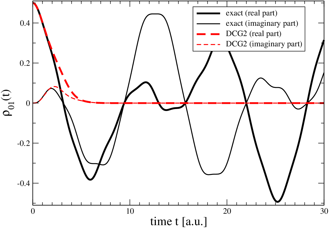
where we will generally observe a decay whenever $\rho_{\rm B}^{00}(1-\rho_{\rm B}^{00})\neq 0$ , see figure 1 (b).

Refer to caption — Figure 1: [Color Online] Comparison of exact (solid black) and DCG2 (dashed red) solutions for the diagonal (a) and off-diagonal (b) matrix elements of the density matrix. Imaginary parts are displayed with thin lines. Naturally, the exact solution displays complete recurrences. For the diagonal matrix elements, this feature is well reproduced by the DCG2 approach, whereas for the off-diagonals only the short-time dynamics is well approximated. The other parameters have been chosen as follows $\lambda=0.25$ , $\omega=1.0$ , $\Omega=2.0$ , and $\rho_{\rm B}^{00}=0.5$ .

III.2 DCG4 for two spins

In order to keep the calculations for DCG4 very simple, we consider

\displaystyle H_{\rm S}=\omega\sigma^{z}_{\rm S}\,,\qquad H_{\rm B}=\Omega\sigma^{z}_{\rm B}\,,\qquad H_{\rm SB}=\lambda\sigma^{x}_{\rm S}\otimes\sigma^{z}_{\rm B}\,,

(33)

where also here the coupling operators are hermitian. In this case, the bath correlation functions are all time-independent, which enables a convenient calculation of the Liouvillian matrix elements. The example is of course a bit trivial, since the exact solution for the reduced density matrix does not depend on $\Omega$ . Note however, that unlike the pure dephasing limit considered in [26] this case still holds some time-dependence that can be found in the system operator in the interaction picture.

The exact solution can be calculated by exponentiating the complete Hamiltonian and tracing out the second spin in the solution for the density matrix as in subsection III.1 and in a similar manner we determine the DCG1, DCG2, DCG3, and DCG4 solutions by directly determining the $4\times 4$ Liouvillian matrix as described in subsection II.4 (not shown). The solution is then obtained by exponentiating the Liouvillian. The resulting solution for the diagonals is displayed in figure 2 (a) and for the off-diagonals in figure 2 (b).

III.3 Spin-Boson model

We consider a single system spin coupled to a bath of bosonic modes ( $\omega_{k}>0$ )

	$\displaystyle H_{\rm S}$	$\displaystyle=$	$\displaystyle\frac{\varepsilon_{\rm d}}{2}\left(\mbox{\boldmath$1$}-\sigma^{z}\right)\,,\qquad H_{\rm B}=\sum_{k}\omega_{k}\left(b_{k}^{\dagger}b_{k}+\frac{1}{2}\right)\,,$
	$\displaystyle H_{\rm SB}$	$\displaystyle=$	$\displaystyle\lambda A\otimes\left[\sum_{k}h_{k}b_{k}+h_{k}^{*}b_{k}^{\dagger}\right]\,,$		(34)

where for simplicity we have restricted ourselves to the case of single-operator coupling, and the operator $A=A^{\dagger}$ will be specified later-on.

We will consider a thermalized initial bath density matrix

\displaystyle\rho_{\rm B}^{0}=\frac{e^{-\beta H_{\rm B}}}{{\rm Tr_{B}}\left\{e^{-\beta H_{\rm B}}\right\}}

(35)

where $\beta=(k_{\rm B}T)^{-1}$ denotes the inverse reservoir temperature.

III.3.1 Bath Correlation Functions

We evaluate the traces in the correlation functions in Eqn. (12) in Fock-space, where the bath density matrix (35) is diagonal. By doing so it becomes obvious that the number of creation and annihilation operators in each term of the bath-bath correlation functions must be balanced for all modes to obtain a nonvanishing result. Therefore, we conclude (since only one operator is involved, we may omit the indices) $C(t_{1})=0=C(t_{1},t_{2},t_{3})$ . In the interaction picture, the annihilation and creation operators transform according to $\mbox{\boldmath$b_{k}$}(t)=e^{+iH_{\rm B}t}b_{k}e^{-iH_{\rm B}t}=e^{-i\omega_{k}t}b_{k}$ and the hermitian conjugate, respectively.

The second order correlation function then evaluates to

$\displaystyle C(t_{1},t_{2})$	$\displaystyle=$	$\displaystyle\frac{1}{2\pi}\int\limits_{0}^{\infty}d\omega G(\omega)\Big\{n(\omega)e^{+i\omega(t_{1}-t_{2})}$	(36)
		$\displaystyle+\left[1+n(\omega)\right]e^{-i\omega(t_{1}-t_{2})}\Big\}$
	$\displaystyle=$	$\displaystyle\frac{1}{2\pi}\int\limits_{-\infty}^{+\infty}\frac{G({\left\|\omega\right\|})}{{\left\|e^{\beta\omega}-1\right\|}}e^{+i\omega(t_{1}-t_{2})}d\omega\,,$

where the bosonic occupation number is given by $n(\omega)=\frac{1}{e^{\beta\omega}-1}$ . In the above equation, we have assumed a quasi-continuous spectral density $G(\omega)=2\pi\sum_{k}{\left|h_{k}\right|}^{2}\delta(\omega-\omega_{k})$ to convert the sum into an integral. When we parametrize the spectral density as

\displaystyle G(\omega)=G_{0}\omega^{S}e^{-\omega/\omega_{\rm c}}\,,

(37)

where $\omega_{\rm c}$ denotes a cutoff frequency and the parameter $S$ governs the slope at $\omega=0$ , we can obtain an analytic solution for the correlation function [27, 28]

	$\displaystyle C(t_{1},t_{2})$	$\displaystyle=$	$\displaystyle\frac{G_{0}\Gamma(1+S)}{2\pi\beta^{1+S}}\Big[\zeta\left(1+S,\frac{1}{\beta\omega_{\rm c}}+i\frac{(t_{1}-t_{2})}{\beta}\right)$		(38)
			$\displaystyle+\zeta\left(1+S,1+\frac{1}{\beta\omega_{\rm c}}-i\frac{(t_{1}-t_{2})}{\beta}\right)\Big]$		(38)

in terms of generalized Riemann Zeta functions $\zeta(x,y)$ .

The next non-vanishing correlation function is fourth order, where we obtain

	$\displaystyle C(t_{1},t_{2},t_{3},t_{4})$	$\displaystyle=$	$\displaystyle C(t_{2},t_{3})C(t_{1},t_{4})+C(t_{1},t_{3})C(t_{2},t_{4})$		(39)
			$\displaystyle+C(t_{1},t_{2})C(t_{3},t_{4})\,,$		(39)

which can for example be obtained using Wicks theorem (for a special case see also Eqn. (61) in [11]).

III.3.2 Pure Dephasing

The case of pure dephasing $A=\sigma^{z}$ is exactly solvable [29, 30] and it is known that DCG2 already yields the exact result [24]. The exact solution predicts time-independent diagonal matrix elements and a decay of the off-diagonal matrix element according to (in the interaction picture, cf. Eqn. (82) in [30] in the limit of a continuous bath spectrum)

	$\displaystyle\mbox{\boldmath$\rho_{01}$}(t)$	$\displaystyle=$	$\displaystyle e^{-\Gamma(t)}\mbox{\boldmath$\rho_{01}$}(0)\,,$
	$\displaystyle\Gamma(t)$	$\displaystyle=$	$\displaystyle\frac{8\lambda^{2}}{2\pi}\int\limits_{0}^{\infty}G(\omega)\frac{\sin^{2}(\omega t/2)}{\omega^{2}}{\coth}\left[\frac{\beta\omega}{2}\right]d\omega\,,$		(40)

where the additional factor of $\frac{1}{2\pi}$ in comparison to [24] results from a different definition of the spectral density $G(\omega)$ . By taking the time derivative of the exact solution density matrix we obtain a closed master equation that is not of Lindblad form (not even with time-dependent coefficients) but nevertheless must – as it is exact – preserve positivity. Hence, one would regard this case as truly non-Markovian [21]. The corresponding steady state is also derived by the equation of motion method in appendix A. For pure dephasing we have $\mbox{\boldmath$A$}(t)=A=\sigma^{z}$ . We observe a decoupled evolution of diagonal and off-diagonal matrix elements of the density matrix.

For the second order contribution we have (using $\Theta(t_{1}-t_{2})+\Theta(t_{2}-t_{1})=1$ ) from Eqn. (13)

\displaystyle\mbox{\boldmath${\cal T}_{2}^{\tau}$}\mbox{\boldmath$\rho_{\rm S}^{0}$}=\int\limits_{0}^{\tau}C(t_{1},t_{2})\left[\sigma^{z}\mbox{\boldmath$\rho_{\rm S}^{0}$}\sigma^{z}-\mbox{\boldmath$\rho_{\rm S}^{0}$}\right]dt_{1}dt_{2}\,,

(41)

from which we obtain

$\displaystyle\left<0\right\|\mbox{\boldmath${\cal T}_{2}^{\tau}$}\mbox{\boldmath$\rho_{\rm S}^{0}$}\left\|0\right>$	$\displaystyle=$	$\displaystyle\left<1\right\|\mbox{\boldmath${\cal T}_{2}^{\tau}$}\mbox{\boldmath$\rho_{\rm S}^{0}$}\left\|1\right>=0\,,$
$\displaystyle\left<0\right\|\mbox{\boldmath${\cal T}_{2}^{\tau}$}\mbox{\boldmath$\rho_{\rm S}^{0}$}\left\|1\right>$	$\displaystyle=$	$\displaystyle-2\int\limits_{0}^{\tau}C(t_{1},t_{2})dt_{1}dt_{2}\mbox{\boldmath$\rho_{\rm S}^{01}$}$
	$\displaystyle=$	$\displaystyle-\frac{8}{2\pi}\int\limits_{0}^{\infty}G(\omega)\frac{\sin^{2}(\omega\tau/2)}{\omega^{2}}\coth\left[\frac{\beta\omega}{2}\right]d\omega\mbox{\boldmath$\rho_{\rm S}^{01}$}\,,$

which leads to the same exponential decay as with the exact solution (40), i.e., as noted earlier [24], DCG2 yields the exact solution in this case. Note that this example demonstrates explicitly that the DCG2 solution cannot be generally written as the solution of a single Lindblad-type master equation with time-dependent coefficients, such that it should be classified as non-Markovian [21].

Using the relation

$\displaystyle 0$	$\displaystyle=$	$\displaystyle+\Theta(t_{4}-t_{3})\Theta(t_{3}-t_{2})\Theta(t_{2}-t_{1})$	(42)
		$\displaystyle+\Theta(t_{3}-t_{4})\Theta(t_{2}-t_{1})$
		$\displaystyle+\Theta(t_{1}-t_{2})\Theta(t_{2}-t_{3})\Theta(t_{3}-t_{4})$
		$\displaystyle-\Theta(t_{2}-t_{3})\Theta(t_{3}-t_{4})-\Theta(t_{3}-t_{2})\Theta(t_{2}-t_{1})\qquad$

we obtain for the fourth order contribution

$\displaystyle\left<0\right\|\mbox{\boldmath${\cal T}_{4}^{\tau}$}\mbox{\boldmath$\rho_{\rm S}^{0}$}\left\|0\right>$	$\displaystyle=$	$\displaystyle\left<1\right\|\mbox{\boldmath${\cal T}_{4}^{\tau}$}\mbox{\boldmath$\rho_{\rm S}^{0}$}\left\|1\right>=0\,,$
$\displaystyle\left<0\right\|\mbox{\boldmath${\cal T}_{4}^{\tau}$}\mbox{\boldmath$\rho_{\rm S}^{0}$}\left\|1\right>$	$\displaystyle=$	$\displaystyle 2\mbox{\boldmath$\rho_{\rm S}^{01}$}\int\limits_{0}^{\tau}dt_{1}dt_{2}dt_{3}dt_{4}C(t_{1},t_{2},t_{3},t_{4})\times$	(43)
		$\displaystyle\Big[\Theta(t_{3}-t_{2})\Theta(t_{2}-t_{1})$
		$\displaystyle+\Theta(t_{2}-t_{3})\Theta(t_{3}-t_{4})\Big]$
	$\displaystyle=$	$\displaystyle 2\int\limits_{0}^{\tau}dt_{1}dt_{2}dt_{3}dt_{4}C(t_{1},t_{2})C(t_{3},t_{4})\mbox{\boldmath$\rho_{\rm S}^{01}$}\,,$

where we have exploited the symmetries of the fourth order correlation functions under exchange of the arguments and the relation

$\displaystyle 2$	$\displaystyle=$	$\displaystyle\Big[+\Theta(t_{2}-t_{3})\Theta(t_{3}-t_{4})+\Theta(t_{3}-t_{2})\Theta(t_{2}-t_{1})\qquad$	(44)
		$\displaystyle+\Theta(t_{1}-t_{2})\Theta(t_{2}-t_{4})+\Theta(t_{2}-t_{1})\Theta(t_{1}-t_{3})$
		$\displaystyle+\Theta(t_{3}-t_{2})\Theta(t_{2}-t_{4})+\Theta(t_{2}-t_{3})\Theta(t_{3}-t_{1})$
		$\displaystyle+\Theta(t_{4}-t_{1})\Theta(t_{1}-t_{2})+\Theta(t_{1}-t_{4})\Theta(t_{4}-t_{3})$
		$\displaystyle+\Theta(t_{3}-t_{4})\Theta(t_{4}-t_{2})+\Theta(t_{4}-t_{3})\Theta(t_{3}-t_{1})$
		$\displaystyle+\Theta(t_{1}-t_{4})\Theta(t_{4}-t_{2})+\Theta(t_{4}-t_{1})\Theta(t_{1}-t_{3})\Big]\,.$

The non-vanishing off-diagonal contribution has to be compared with the counter-term arising from the second order

$\displaystyle\frac{1}{2}\left<0\right\|\mbox{\boldmath${\cal T}_{2}^{\tau}$}[\mbox{\boldmath${\cal T}_{2}^{\tau}$}\mbox{\boldmath$\rho_{\rm S}^{0}$}]\left\|1\right>$	$\displaystyle=$	$\displaystyle\frac{1}{2}\left[-2\int\limits_{0}^{\tau}C(t_{1},t_{2})dt_{1}dt_{2}\right]^{2}\mbox{\boldmath$\rho_{\rm S}^{01}$}$	(45)
	$\displaystyle=$	$\displaystyle 2\left[\int\limits_{0}^{\tau}C(t_{1},t_{2})dt_{1}dt_{2}\right]\times$
		$\displaystyle\left[\int\limits_{0}^{\tau}C(t_{3},t_{4})dt_{3}dt_{4}\right]\mbox{\boldmath$\rho_{\rm S}^{01}$}$

Since the diagonal elements of the density matrix are neither affected by ${\cal T}_{2}^{\tau}$ nor by ${\cal T}_{4}^{\tau}$ we conclude that we have for pure dephasing

\displaystyle\mbox{\boldmath${\cal T}_{4}^{\tau}$}=\frac{1}{2}\mbox{\boldmath${\cal T}_{2}^{\tau}$}\mbox{\boldmath${\cal T}_{2}^{\tau}$}\,,

(46)

such that DCG4 will yield the same result as DCG2. Since DCG2 is already exact for this case, this cancellation is a strong indicator for the correctness of our fourth order correlation function (39).

III.3.3 Dissipation

We are now in a position to apply DCG to more interesting coupling operators (picking up a time-dependence in the interaction picture) that also affect the evolution of the diagonal elements of the density matrix. Transforming $A=\sigma^{x}$ into the interaction picture we obtain $\mbox{\boldmath$A$}(t)=\cos(\varepsilon_{\rm d}t)\sigma^{x}+\sin(\varepsilon_{\rm d}t)\sigma^{y}$ . Inserting this result we find for the second order term in Eqn. (13)

	$\displaystyle\left<0\right\|\mbox{\boldmath${\cal T}_{2}^{\tau}$}[\mbox{\boldmath$\rho_{\rm S}$}]\left\|0\right>$	$\displaystyle=$	$\displaystyle\int\limits_{0}^{\tau}dt_{1}dt_{2}C(t_{1},t_{2})\Big[-e^{-i\varepsilon_{\rm d}(t_{1}-t_{2})}\mbox{\boldmath$\rho_{\rm S}^{00}$}+e^{+i\varepsilon_{\rm d}(t_{1}-t_{2})}\mbox{\boldmath$\rho_{\rm S}^{11}$}\Big]\,,$
	$\displaystyle\left<0\right\|\mbox{\boldmath${\cal T}_{2}^{\tau}$}[\mbox{\boldmath$\rho_{\rm S}$}]\left\|1\right>$	$\displaystyle=$	$\displaystyle\int\limits_{0}^{\tau}dt_{1}dt_{2}C(t_{1},t_{2})\Big[-\Theta(t_{2}-t_{1})e^{+i\varepsilon_{\rm d}(t_{1}-t_{2})}\mbox{\boldmath$\rho_{\rm S}^{01}$}-\Theta(t_{1}-t_{2})e^{-i\varepsilon_{\rm d}(t_{1}-t_{2})}\mbox{\boldmath$\rho_{\rm S}^{01}$}+e^{-i\varepsilon_{\rm d}(t_{1}+t_{2})}\mbox{\boldmath$\rho_{\rm S}^{10}$}\Big]$		(47)

and similarly for the other terms, such that by arranging the matrix elements of the $2\times 2$ density matrix in a 4-dimensional vector as $(\mbox{\boldmath$\rho_{\rm S}^{00}$},\mbox{\boldmath$\rho_{\rm S}^{01}$},\mbox{\boldmath$\rho_{\rm S}^{10}$},\mbox{\boldmath$\rho_{\rm S}^{11}$})$ we find the matrix elements of the corresponding $4\times 4$ superoperator to be

\displaystyle\mbox{\boldmath${\cal T}_{2}^{\tau}$}=\int\limits_{0}^{\tau}C(t_{1},t_{2})\left(\begin{array}[]{cccc}-e^{-i\varepsilon_{\rm d}(t_{1}-t_{2})}&0&0&+e^{+i\varepsilon_{\rm d}(t_{1}-t_{2})}\\ 0&-e^{-i\varepsilon_{\rm d}{\left|t_{1}-t_{2}\right|}}&+e^{-i\varepsilon_{\rm d}(t_{1}+t_{2})}&0\\ 0&+e^{+i\varepsilon_{\rm d}(t_{1}+t_{2})}&-e^{+i\varepsilon_{\rm d}{\left|t_{1}-t_{2}\right|}}&0\\ +e^{-i\varepsilon_{\rm d}(t_{1}-t_{2})}&0&0&-e^{+i\varepsilon_{\rm d}(t_{1}-t_{2})}\end{array}\right)dt_{1}dt_{2}\,,

such that we observe a decoupled evolution of diagonal and off-diagonal matrix elements. Defining

$\displaystyle m_{11}(\tau)$	$\displaystyle\equiv$	$\displaystyle\left(\mbox{\boldmath${\cal T}_{2}^{\tau}$}\right)_{11}$
	$\displaystyle=$	$\displaystyle-\frac{\tau^{2}}{2\pi}\int\limits_{-\infty}^{+\infty}\frac{G({\left\|\omega\right\|})}{{\left\|e^{\beta\omega}-1\right\|}}{\rm sinc}^{2}\left[(\omega-\varepsilon_{\rm d})\frac{\tau}{2}\right]d\omega\,,$
$\displaystyle m_{14}(\tau)$	$\displaystyle\equiv$	$\displaystyle\left(\mbox{\boldmath${\cal T}_{2}^{\tau}$}\right)_{14}$
	$\displaystyle=$	$\displaystyle+\frac{\tau^{2}}{2\pi}\int\limits_{-\infty}^{+\infty}\frac{G({\left\|\omega\right\|})}{{\left\|e^{\beta\omega}-1\right\|}}{\rm sinc}^{2}\left[(\omega+\varepsilon_{\rm d})\frac{\tau}{2}\right]d\omega\,,$
$\displaystyle m_{41}(\tau)$	$\displaystyle\equiv$	$\displaystyle\left(\mbox{\boldmath${\cal T}_{2}^{\tau}$}\right)_{41}=-m_{11}(\tau)\,,$
$\displaystyle m_{44}(\tau)$	$\displaystyle\equiv$	$\displaystyle\left(\mbox{\boldmath${\cal T}_{2}^{\tau}$}\right)_{44}=-m_{14}(\tau)$	(53)

we obtain the second order solution for the diagonals (using trace conservation)

	$\displaystyle\rho_{00}^{\tau}(\tau)$	$\displaystyle=$	$\displaystyle\rho_{00}^{0}\exp\left[\lambda^{2}\left(m_{11}(\tau)-m_{14}(\tau)\right)\right]$		(54)
			$\displaystyle+\frac{1-\exp\left[\lambda^{2}\left(m_{11}(\tau)-m_{14}(\tau)\right)\right]}{1-\frac{m_{11}(\tau)}{m_{14}(\tau)}}\,.$		(54)

In Eqn. (53) it is already obvious that for finite times $\tau$ all frequencies will contribute to the matrix elements $m_{ij}(\tau)$ in contrast to the Markov approximation, where only $G(\varepsilon_{\rm d})$ is relevant. With using that the bandfilter sinc functions transform into Dirac-Delta functions in Eqn. (24) we can perform the limit $\tau\to\infty$ to obtain the steady state

\displaystyle\rho_{00}^{\infty}=\frac{1}{1+e^{-\beta\varepsilon_{\rm d}}}\,,

(55)

which corresponds to the thermalized system density matrix that consistent with our expectations, compare also appendix A. The same stationary state can also be obtained by using the method of equation of motion and truncating correlations at second order between system and reservoir.

The Markovian limit is obtained by using

	$\displaystyle m_{11}^{\rm MK}(t)=t\lim_{\tau\to\infty}\frac{1}{\tau}m_{11}(\tau)=-tG({\left\|\varepsilon_{\rm d}\right\|}){\left\|n(+\varepsilon_{\rm d})\right\|}\,,$
	$\displaystyle m_{14}^{\rm MK}(t)=t\lim_{\tau\to\infty}\frac{1}{\tau}m_{14}(\tau)=+tG({\left\|\varepsilon_{\rm d}\right\|}){\left\|n(-\varepsilon_{\rm d})\right\|}\,,$		(56)

where we have again used identity (24) in Eqn. (53). Evidently, the above equation leads to the same steady state as the Born-Markov approximation (55).

By virtue of Eqn. (42) and using that $\left[C(t_{1},t_{2},t_{3},t_{4})=C(t_{4},t_{3},t_{2},t_{1})\right]^{*}$ we obtain for the diagonal part

$\displaystyle\left<0\right\|\mbox{\boldmath${\cal T}_{4}^{\tau}$}\mbox{\boldmath$\rho_{\rm S}^{0}$}\left\|0\right>$	$\displaystyle=$	$\displaystyle 2\int\limits_{0}^{\tau}\Re\left\{C(t_{1},t_{2},t_{3},t_{4})e^{-i\varepsilon_{\rm d}(t_{1}-t_{2}+t_{3}-t_{4})}\right\}\times$	(57)
		$\displaystyle\Theta(t_{2}-t_{3})\Theta(t_{3}-t_{4})dt_{1}dt_{2}dt_{3}dt_{4}\mbox{\boldmath$\rho_{\rm S}^{00}$}$
		$\displaystyle-2\int\limits_{0}^{\tau}\Re\left\{C(t_{1},t_{2},t_{3},t_{4})e^{+i\varepsilon_{\rm d}(t_{1}-t_{2}+t_{3}-t_{4})}\right\}\times$
		$\displaystyle\Theta(t_{2}-t_{3})\Theta(t_{3}-t_{4})dt_{1}dt_{2}dt_{3}dt_{4}\mbox{\boldmath$\rho_{\rm S}^{11}$}$
	$\displaystyle\equiv$	$\displaystyle p_{11}(\tau)\mbox{\boldmath$\rho_{\rm S}^{00}$}+p_{14}(\tau)\mbox{\boldmath$\rho_{\rm S}^{11}$}\,.$

This result has to be combined with the counterterm arising from the squared second order contribution. Defining

$\displaystyle\tilde{p}_{11}(\tau)$	$\displaystyle=$	$\displaystyle\lambda^{2}m_{11}(\tau)-\frac{\lambda^{4}}{2}\left[m_{11}(\tau)m_{11}(\tau)+m_{14}(\tau)m_{41}(\tau)\right]$
		$\displaystyle+\lambda^{4}p_{11}(\tau)\,,$
$\displaystyle\tilde{p}_{14}(\tau)$	$\displaystyle=$	$\displaystyle\lambda^{2}m_{14}(\tau)-\frac{\lambda^{4}}{2}\left[m_{11}(\tau)m_{14}(\tau)+m_{14}(\tau)m_{44}(\tau)\right]$	(58)
		$\displaystyle+\lambda^{4}p_{14}(\tau)\,,$	(58)

we therefore obtain the fourth order solution

	$\displaystyle\rho_{00}^{\tau}(\tau)$	$\displaystyle=$	$\displaystyle\rho_{00}^{0}\exp\left[\tilde{p}_{11}(\tau)-\tilde{p}_{14}(\tau)\right]$		(59)
			$\displaystyle+\frac{1-\exp\left[\tilde{p}_{11}(\tau)-\tilde{p}_{14}(\tau)\right]}{1-\frac{\tilde{p}_{11}(\tau)}{\tilde{p}_{14}(\tau)}}\,.$		(59)

A general exact solution is unfortunately not available for this case. However, it is interesting to note that when considering the Markov limit $\beta=0$ , $\omega_{\rm c}\to\infty$ , and $S=0$ (where the Markov approximation becomes exact) the correlation function (36) becomes a $\delta$ -function and we see that in this limit, the fourth order term is cancelled by the squared second order counter term. For comparison, we plot Born-Markov solution, DCG2, and DCG4 solutions in figure 3

For the dissipative spin-boson model and Ohmic dissipation ( $S=1$ ) one obtains an exponential decay of the expectation value $\left<\sigma^{x}\right>(t)$ in the long time limit [31] (note the rotation $\sigma^{z}\to\sigma^{x}$ and $\sigma^{x}\to-\sigma^{z}$ ). This corresponds to a decay of the off-diagonal matrix elements and is of course also reproduced by the DCG approach.

III.4 Fano-Anderson Model

We consider the Fano-Anderson model [32, 33]: two leads that are connected by a single quantum dot, through which electrons may tunnel from one lead to the other. The Hamiltonian is given by

$\displaystyle H$	$\displaystyle=$	$\displaystyle H_{\rm S}+H_{\rm B}+H_{\rm SB}\,,$
$\displaystyle H_{\rm S}$	$\displaystyle=$	$\displaystyle\varepsilon_{\rm d}d^{\dagger}d\,,\;\;H_{\rm B}=\sum_{ka}\omega_{ka}c_{ka}^{\dagger}c_{ka}\,,$
$\displaystyle H_{\rm SB}$	$\displaystyle=$	$\displaystyle\lambda\sum_{ka}\left[t_{ka}dc_{ka}^{\dagger}-t_{ka}^{*}d^{\dagger}c_{ka}\right]$	(60)

with fermionic operators creating an alectron with momentum $k$ in the left or right lead $a\in\{\rm L,R\}$ for $c_{ka}^{\dagger}$ or in the quantum dot $d^{\dagger}$ . Due to the fermionic anticommutation relations, the model (60) can be solved exactly for example with Greens functions [34, 35]. We provide a simplified derivation based on the equation of motion method in appendix B.

In contrast to our assumptions in section II, the operators $d$ and $c_{ka}$ do not act on separate Hilbert spaces, which is evident from their anticommutation relations $\left\{d,c_{ka}^{\dagger}\right\}=0$ . This becomes even more explicit via the decomposition

	$\displaystyle d$	$\displaystyle=$	$\displaystyle\left\|0\right>\left<1\right\|\otimes\mbox{\boldmath$1$}\,,$
	$\displaystyle c_{ka}$	$\displaystyle=$	$\displaystyle\left[\left\|0\right>\left<0\right\|-\left\|1\right>\left<1\right\|\right]\otimes\bar{c}_{ka}\,,$		(61)

where $\left|0\right>$ and $\left|1\right>$ denote the empty and filled dot states, respectively, and the fermionic operators $\bar{c}_{ka}$ act only on the (distinct) Fock space of the remaining sites in the leads with $\left\{\bar{c}_{ka},\bar{c}_{k^{\prime}a^{\prime}}^{\dagger}\right\}=\delta_{kk^{\prime}}\delta_{aa^{\prime}}$ . Naturally, the above decomposition obeys the original anticommutation relations such as $\left\{d,c_{ka}\right\}=0$ and we conclude for the operators in the interaction Hamiltonian $dc_{ka}^{\dagger}=-\left|0\right>\left<1\right|\otimes\bar{c}_{ka}^{\dagger}$ , and $d^{\dagger}c_{ka}=+\left|1\right>\left<0\right|\otimes\bar{c}_{ka}$ , such that now the new operators commute by construction. Similiar decompositions are also possible systems containing more than one site. We identify

	$\displaystyle A_{1}$	$\displaystyle=$	$\displaystyle-\left\|0\right>\left<1\right\|\,,\qquad A_{2}=-\left\|1\right>\left<0\right\|\,,$
	$\displaystyle B_{1}$	$\displaystyle=$	$\displaystyle\sum_{ka}t_{ka}\bar{c}_{ka}^{\dagger}\,,\qquad B_{2}=\sum_{ka}t_{ka}^{*}\bar{c}_{ka}\,.$		(62)

We assume that there are no correlations between left and right leads. Here we will just consider the infinite bias limit (although this is not crucial, it enables for an analytic calculation of all integrals): Taking the chemical potentials to plus or minus infinity for the left and right leads, respectively ( $\mu_{\rm L}\to+\infty$ and $\mu_{\rm R}\to-\infty$ ), we obtain for the fermionic occupation number

	$\displaystyle\left<\bar{c}_{k\rm L}^{\dagger}\bar{c}_{k\rm L}\right>$	$\displaystyle=$	$\displaystyle\frac{1}{e^{\beta(\omega_{k}-\mu_{\rm L})}+1}\to 1\,,$
	$\displaystyle\left<\bar{c}_{k\rm R}^{\dagger}\bar{c}_{k\rm R}\right>$	$\displaystyle=$	$\displaystyle\frac{1}{e^{\beta(\omega_{k}-\mu_{\rm R})}+1}\to 0\,.$		(63)

We observe that the coupling operators are non-hermitian in this case. The correlation functions relevant for the evolution of the diagonal matrix elements can be calculated by introducing continuum tunneling rates via $\Gamma_{a}(\omega)\equiv 2\pi\sum_{k}{\left|t_{ka}\right|}^{2}\delta(\omega-\omega_{ka})$

$\displaystyle C_{\rm L}(t_{1}-t_{2})\equiv C_{12}(t_{1},t_{2})$	$\displaystyle=$	$\displaystyle\frac{1}{2\pi}\int\limits_{-\infty}^{+\infty}\Gamma_{\rm L}(\omega)e^{+i\omega(t_{1}-t_{2})}d\omega\,,$
$\displaystyle C_{\rm R}(t_{2}-t_{1})\equiv C_{21}(t_{1},t_{2})$	$\displaystyle=$	$\displaystyle\frac{1}{2\pi}\int\limits_{-\infty}^{+\infty}\Gamma_{\rm R}(\omega)e^{-i\omega(t_{1}-t_{2})}d\omega\,,$
$\displaystyle C_{1212}(t_{1},t_{2},t_{3},t_{4})$	$\displaystyle=$	$\displaystyle C_{\rm L}(t_{1}-t_{2})C_{\rm L}(t_{3}-t_{4})$
		$\displaystyle+C_{\rm L}(t_{1}-t_{4})C_{\rm R}(t_{3}-t_{2})\,,$
$\displaystyle C_{2121}(t_{1},t_{2},t_{3},t_{4})$	$\displaystyle=$	$\displaystyle C_{\rm R}(t_{2}-t_{1})C_{\rm R}(t_{4}-t_{3})$	(64)
		$\displaystyle+C_{\rm R}(t_{4}-t_{1})C_{\rm L}(t_{2}-t_{3})\,.$	(64)

From Eqn. (13), we can derive the second order approximation

${\cal T}_{2}^{\tau}$ $\rho_{\rm S}^{0}$	$\displaystyle=$	$\displaystyle\int\limits_{0}^{\tau}dt_{1}dt_{2}\Big[-C_{21}(t_{1},t_{2})\Theta(t_{2}-t_{1})\mbox{\boldmath$\rho_{\rm S}^{0}$}\mbox{\boldmath$A_{1}^{\dagger}$}(t_{1})\mbox{\boldmath$A_{2}^{\dagger}$}(t_{2})-C_{12}(t_{1},t_{2})\Theta(t_{2}-t_{1})\mbox{\boldmath$\rho_{\rm S}^{0}$}\mbox{\boldmath$A_{2}^{\dagger}$}(t_{1})\mbox{\boldmath$A_{1}^{\dagger}$}(t_{2})$	(65)
		$\displaystyle+C_{21}(t_{1},t_{2})\mbox{\boldmath$A_{1}$}(t_{2})\mbox{\boldmath$\rho_{\rm S}^{0}$}\mbox{\boldmath$A_{1}^{\dagger}$}(t_{1})+C_{12}(t_{1},t_{2})\mbox{\boldmath$A_{2}$}(t_{2})\mbox{\boldmath$\rho_{\rm S}^{0}$}\mbox{\boldmath$A_{2}^{\dagger}$}(t_{1})$
		$\displaystyle-C_{12}(t_{1},t_{2})\Theta(t_{1}-t_{2})\mbox{\boldmath$A_{1}$}(t_{1})\mbox{\boldmath$A_{2}$}(t_{2})\mbox{\boldmath$\rho_{\rm S}^{0}$}-C_{21}(t_{1},t_{2})\Theta(t_{1}-t_{2})\mbox{\boldmath$A_{2}$}(t_{1})\mbox{\boldmath$A_{1}$}(t_{2})\mbox{\boldmath$\rho_{\rm S}^{0}$}\Big]$
	$\displaystyle=$	$\displaystyle\int\limits_{-\infty}^{+\infty}\frac{d\omega}{2\pi}\Gamma_{\rm R}(\omega)\int\limits_{0}^{\tau}dt_{1}dt_{2}e^{-i(\omega-\varepsilon_{\rm d})(t_{1}-t_{2})}\left[-\mbox{\boldmath$\rho_{\rm S}^{0}$}\left\|1\right>\left<1\right\|\Theta(t_{2}-t_{1})+\left\|0\right>\left<1\right\|\mbox{\boldmath$\rho_{\rm S}^{0}$}\left\|1\right>\left<0\right\|-\left\|1\right>\left<1\right\|\mbox{\boldmath$\rho_{\rm S}^{0}$}\Theta(t_{1}-t_{2})\right]$
		$\displaystyle+\int\limits_{-\infty}^{+\infty}\frac{d\omega}{2\pi}\Gamma_{\rm L}(\omega)\int\limits_{0}^{\tau}dt_{1}dt_{2}e^{+i(\omega-\varepsilon_{\rm d})(t_{1}-t_{2})}\left[-\mbox{\boldmath$\rho_{\rm S}^{0}$}\left\|0\right>\left<0\right\|\Theta(t_{2}-t_{1})+\left\|1\right>\left<0\right\|\mbox{\boldmath$\rho_{\rm S}^{0}$}\left\|0\right>\left<1\right\|-\left\|0\right>\left<0\right\|\mbox{\boldmath$\rho_{\rm S}^{0}$}\Theta(t_{1}-t_{2})\right]\,,$

from which we can infer the matrix elements of the second-order Liouvillian via $\mbox{\boldmath${\cal L}_{2}^{\tau}$}\mbox{\boldmath$\rho_{\rm S}^{0}$}=\frac{1}{\tau}\mbox{\boldmath${\cal T}_{2}^{\tau}$}\mbox{\boldmath$\rho_{\rm S}^{0}$}$ . The Born-Markov-secular approximation is obtained by the Liouvillian ${\cal L}_{2}^{\infty}$ with the help of Eqn (24).

When we parametrize the tunneling rates by Lorentzians [36]

\displaystyle\Gamma_{\rm R}(\omega)=\frac{\Gamma_{\rm R}^{0}\delta_{\rm R}^{2}}{\left(\omega-\epsilon_{\rm R}\right)^{2}+\delta_{\rm R}^{2}}\,,\;\;\Gamma_{\rm L}(\omega)=\frac{\Gamma_{\rm L}^{0}\delta_{\rm L}^{2}}{\left(\omega-\epsilon_{\rm L}\right)^{2}+\delta_{\rm L}^{2}}\,,\qquad

(66)

we obtain an analytic expression for the bath correlation functions in terms of a single decaying exponential

\displaystyle C_{\rm R}(t)=\frac{\Gamma_{\rm R}^{0}\delta_{\rm R}}{2}e^{-{\left|t\right|}\delta_{\rm R}+i\epsilon_{\rm R}t}\,,\;\;C_{\rm L}(t)=\frac{\Gamma_{\rm L}^{0}\delta_{\rm L}}{2}e^{-{\left|t\right|}\delta_{\rm L}+i\epsilon_{\rm L}t}\,,\qquad

(67)

such that we can analytically calculate the matrix elements of ${\cal T}_{2}^{\tau}$ that govern the evolution of the diagonals

	$\displaystyle\left(\begin{array}[]{cc}m_{11}(\tau)&m_{14}(\tau)\\ m_{41}(\tau)&m_{44}(\tau)\end{array}\right)$	$\displaystyle\equiv$	$\displaystyle\int\limits_{0}^{\tau}dt_{1}dt_{2}e^{-i\varepsilon_{\rm d}(t_{1}-t_{2})}\times$
			$\displaystyle\left(\begin{array}[]{cc}-C_{\rm L}(t_{1}-t_{2})&+C_{\rm R}(t_{1}-t_{2})\\ +C_{\rm L}(t_{1}-t_{2})&-C_{\rm R}(t_{1}-t_{2})\end{array}\right)\,.$

Then, we obtain from $\left<0\right|\mbox{\boldmath${\cal T}_{2}^{\tau}$}\mbox{\boldmath$\rho_{\rm S}^{0}$}\left|0\right>$ for the evolution of the diagonal matrix element

\dot{\rho}_{00}^{\tau}

\displaystyle=

\displaystyle\lambda^{2}\left[\frac{m_{11}(\tau)}{\tau}\mbox{\boldmath$\rho_{00}^{\tau}$}(t)+\frac{m_{14}(\tau)}{\tau}\mbox{\boldmath$\rho_{11}^{\tau}$}(t)\right]\,,

(74)

where we can exploit trace conservation $\mbox{\boldmath$\rho_{11}^{\tau}$}(t)=1-\mbox{\boldmath$\rho_{00}^{\tau}$}(t)$ (this feature is trivially fulfilled by the coarse-graining approach). Afterwards, the above equation can explicitly be solved for

	$\displaystyle\mbox{\boldmath$\rho_{00}^{\tau}$}(t)$	$\displaystyle=$	$\displaystyle\mbox{\boldmath$\rho_{00}$}(0)\exp\left\{\lambda^{2}\left[m_{11}(\tau)-m_{14}(\tau)\right]\frac{t}{\tau}\right]$		(75)
			$\displaystyle+\frac{1-\exp\left\{\lambda^{2}\left[m_{11}(\tau)-m_{14}(\tau)\right]\frac{t}{\tau}\right\}}{1-\frac{m_{11}(\tau)}{m_{14}(\tau)}}$		(75)

For the fourth-order contribution we obtain (extensively using $C_{\bar{1}\bar{2}\bar{1}\bar{2}}(t_{1},t_{2},t_{3},t_{4})=C_{2121}(t_{1},t_{2},t_{3},t_{4})$ , $C_{1112}(t_{1},t_{2},t_{3},t_{4})=0$ etc.)

${\cal T}_{4}^{\tau}$ $\rho_{\rm S}^{0}$	$\displaystyle=$	$\displaystyle\int\limits_{0}^{\tau}dt_{1}dt_{2}dt_{3}dt_{4}\Big[+C_{2121}(t_{1},t_{2},t_{3},t_{4})\Theta(t_{4}-t_{3})\Theta(t_{3}-t_{2})\Theta(t_{2}-t_{1})\mbox{\boldmath$\rho_{\rm S}^{0}$}\mbox{\boldmath$A_{1}^{\dagger}$}(t_{1})\mbox{\boldmath$A_{2}^{\dagger}$}(t_{2})\mbox{\boldmath$A_{1}^{\dagger}$}(t_{3})\mbox{\boldmath$A_{2}^{\dagger}$}(t_{4})$	(76)
		$\displaystyle+C_{1212}(t_{1},t_{2},t_{3},t_{4})\Theta(t_{4}-t_{3})\Theta(t_{3}-t_{2})\Theta(t_{2}-t_{1})\mbox{\boldmath$\rho_{\rm S}^{0}$}\mbox{\boldmath$A_{2}^{\dagger}$}(t_{1})\mbox{\boldmath$A_{1}^{\dagger}$}(t_{2})\mbox{\boldmath$A_{2}^{\dagger}$}(t_{3})\mbox{\boldmath$A_{1}^{\dagger}$}(t_{4})$
		$\displaystyle-C_{2121}(t_{1},t_{2},t_{3},t_{4})\Theta(t_{3}-t_{2})\Theta(t_{2}-t_{1})\mbox{\boldmath$A_{1}$}(t_{4})\mbox{\boldmath$\rho_{\rm S}^{0}$}\mbox{\boldmath$A_{1}^{\dagger}$}(t_{1})\mbox{\boldmath$A_{2}^{\dagger}$}(t_{2})\mbox{\boldmath$A_{1}^{\dagger}$}(t_{3})$
		$\displaystyle-C_{1212}(t_{1},t_{2},t_{3},t_{4})\Theta(t_{3}-t_{2})\Theta(t_{2}-t_{1})\mbox{\boldmath$A_{2}$}(t_{4})\mbox{\boldmath$\rho_{\rm S}^{0}$}\mbox{\boldmath$A_{2}^{\dagger}$}(t_{1})\mbox{\boldmath$A_{1}^{\dagger}$}(t_{2})\mbox{\boldmath$A_{2}^{\dagger}$}(t_{3})$
		$\displaystyle+C_{2112}(t_{1},t_{2},t_{3},t_{4})\Theta(t_{3}-t_{4})\Theta(t_{2}-t_{1})\mbox{\boldmath$A_{1}$}(t_{3})\mbox{\boldmath$A_{2}$}(t_{4})\mbox{\boldmath$\rho_{\rm S}^{0}$}\mbox{\boldmath$A_{1}^{\dagger}$}(t_{1})\mbox{\boldmath$A_{2}^{\dagger}$}(t_{2})$
		$\displaystyle+C_{2121}(t_{1},t_{2},t_{3},t_{4})\Theta(t_{3}-t_{4})\Theta(t_{2}-t_{1})\mbox{\boldmath$A_{2}$}(t_{3})\mbox{\boldmath$A_{1}$}(t_{4})\mbox{\boldmath$\rho_{\rm S}^{0}$}\mbox{\boldmath$A_{1}^{\dagger}$}(t_{1})\mbox{\boldmath$A_{2}^{\dagger}$}(t_{2})$
		$\displaystyle+C_{1212}(t_{1},t_{2},t_{3},t_{4})\Theta(t_{3}-t_{4})\Theta(t_{2}-t_{1})\mbox{\boldmath$A_{1}$}(t_{3})\mbox{\boldmath$A_{2}$}(t_{4})\mbox{\boldmath$\rho_{\rm S}^{0}$}\mbox{\boldmath$A_{2}^{\dagger}$}(t_{1})\mbox{\boldmath$A_{1}^{\dagger}$}(t_{2})$
		$\displaystyle+C_{1221}(t_{1},t_{2},t_{3},t_{4})\Theta(t_{3}-t_{4})\Theta(t_{2}-t_{1})\mbox{\boldmath$A_{2}$}(t_{3})\mbox{\boldmath$A_{1}$}(t_{4})\mbox{\boldmath$\rho_{\rm S}^{0}$}\mbox{\boldmath$A_{2}^{\dagger}$}(t_{1})\mbox{\boldmath$A_{1}^{\dagger}$}(t_{2})$
		$\displaystyle-C_{2121}(t_{1},t_{2},t_{3},t_{4})\Theta(t_{2}-t_{3})\Theta(t_{3}-t_{4})\mbox{\boldmath$A_{1}$}(t_{2})\mbox{\boldmath$A_{2}$}(t_{3})\mbox{\boldmath$A_{1}$}(t_{4})\mbox{\boldmath$\rho_{\rm S}^{0}$}\mbox{\boldmath$A_{1}^{\dagger}$}(t_{1})$
		$\displaystyle-C_{1212}(t_{1},t_{2},t_{3},t_{4})\Theta(t_{2}-t_{3})\Theta(t_{3}-t_{4})\mbox{\boldmath$A_{2}$}(t_{2})\mbox{\boldmath$A_{1}$}(t_{3})\mbox{\boldmath$A_{2}$}(t_{4})\mbox{\boldmath$\rho_{\rm S}^{0}$}\mbox{\boldmath$A_{2}^{\dagger}$}(t_{1})$
		$\displaystyle+C_{1212}(t_{1},t_{2},t_{3},t_{4})\Theta(t_{1}-t_{2})\Theta(t_{2}-t_{3})\Theta(t_{3}-t_{4})\mbox{\boldmath$A_{1}$}(t_{1})\mbox{\boldmath$A_{2}$}(t_{2})\mbox{\boldmath$A_{1}$}(t_{3})\mbox{\boldmath$A_{2}$}(t_{4})\mbox{\boldmath$\rho_{\rm S}^{0}$}$
		$\displaystyle+C_{2121}(t_{1},t_{2},t_{3},t_{4})\Theta(t_{1}-t_{2})\Theta(t_{2}-t_{3})\Theta(t_{3}-t_{4})\mbox{\boldmath$A_{2}$}(t_{1})\mbox{\boldmath$A_{1}$}(t_{2})\mbox{\boldmath$A_{2}$}(t_{3})\mbox{\boldmath$A_{1}$}(t_{4})\mbox{\boldmath$\rho_{\rm S}^{0}$}\Big]\,.$

The relevant part in above equation for the evolution of the diagonals evaluates by using Eqn. (42) to

$\displaystyle\left(\mbox{\boldmath${\cal T}_{4}^{\tau}$}\mbox{\boldmath$\rho_{\rm S}^{0}$}\right)_{11}$	$\displaystyle\equiv$	$\displaystyle p_{11}(\tau)\mbox{\boldmath$\rho_{00}^{\tau}$}(t)+p_{14}(\tau)\mbox{\boldmath$\rho_{11}^{\tau}$}(t)\,,$
$\displaystyle p_{11}(\tau)$	$\displaystyle=$	$\displaystyle+\int\limits_{0}^{\tau}dt_{1}dt_{2}dt_{3}dt_{4}e^{-i\varepsilon_{\rm d}(+t_{1}-t_{2}+t_{3}-t_{4})}\times$
		$\displaystyle\left[C_{\rm L}(t_{1}-t_{2})C_{\rm L}(t_{3}-t_{4})+C_{\rm L}(t_{1}-t_{4})C_{\rm R}(t_{3}-t_{2})\right]\left[\Theta(t_{3}-t_{2})\Theta(t_{2}-t_{1})+\Theta(t_{2}-t_{3})\Theta(t_{3}-t_{4})\right]\qquad$
$\displaystyle p_{14}(\tau)$	$\displaystyle=$	$\displaystyle-\int\limits_{0}^{\tau}dt_{1}dt_{2}dt_{3}dt_{4}e^{+i\varepsilon_{\rm d}(t_{1}-t_{2}+t_{3}-t_{4})}\times$	(77)
		$\displaystyle\left[C_{\rm R}(t_{2}-t_{1})C_{\rm R}(t_{4}-t_{3})+C_{\rm R}(t_{4}-t_{1})C_{\rm L}(t_{2}-t_{3})\right]\left[\Theta(t_{3}-t_{2})\Theta(t_{2}-t_{1})+\Theta(t_{2}-t_{3})\Theta(t_{3}-t_{4})\right]\,,$	(77)

where again all integrals can be solved analytically yielding even lengthier expressions than before. Together with

	$\displaystyle\left<0\right\|\mbox{\boldmath${\cal T}_{2}^{\tau}$}\mbox{\boldmath${\cal T}_{2}^{\tau}$}\mbox{\boldmath$\rho_{\rm S}^{0}$}\left\|0\right>$	$\displaystyle=$	$\displaystyle\left[m_{11}(\tau)m_{11}(\tau)+m_{14}(\tau)m_{41}(\tau)\right]\mbox{\boldmath$\rho_{\rm S}^{00}$}$
		$\displaystyle+$	$\displaystyle\left[m_{11}(\tau)m_{14}(\tau)+m_{14}(\tau)m_{44}(\tau)\right]\mbox{\boldmath$\rho_{\rm S}^{11}$}$

we obtain from

	$\displaystyle\lambda^{2}\mbox{\boldmath${\cal L}^{\tau}_{2}$}+\lambda^{4}\mbox{\boldmath${\cal L}^{\tau}_{4}$}$	$\displaystyle=$	$\displaystyle\frac{\lambda^{2}}{\tau}\mbox{\boldmath${\cal T}_{2}^{\tau}$}+\frac{\lambda^{4}}{\tau}\left(\mbox{\boldmath${\cal T}_{4}^{\tau}$}-\frac{\tau^{2}}{2}\mbox{\boldmath${\cal L}^{\tau}_{2}$}\mbox{\boldmath${\cal L}^{\tau}_{2}$}\right)$		(78)
		$\displaystyle=$	$\displaystyle\frac{1}{\tau}\left(\lambda^{2}\mbox{\boldmath${\cal T}_{2}^{\tau}$}+\lambda^{4}\mbox{\boldmath${\cal T}_{4}^{\tau}$}-\frac{\lambda^{4}}{2}\mbox{\boldmath${\cal T}_{2}^{\tau}$}\mbox{\boldmath${\cal T}_{2}^{\tau}$}\right)$		(78)

the following differential equation for the diagonals

$\dot{\rho}_{00}^{\tau}$	$\displaystyle=$	$\displaystyle\frac{1}{\tau}\Big\{\lambda^{2}m_{11}(\tau)-\frac{\lambda^{4}}{2}\Big[m_{11}(\tau)m_{11}(\tau)$	(79)
		$\displaystyle+m_{14}(\tau)m_{41}(\tau)\Big]+\lambda^{4}p_{11}(\tau)\Big\}\mbox{\boldmath$\rho_{00}^{\tau}$}(t)$
		$\displaystyle+\frac{1}{\tau}\Big\{\lambda^{2}m_{14}(\tau)-\frac{\lambda^{4}}{2}\Big[m_{11}(\tau)m_{14}(\tau)$
		$\displaystyle+m_{14}(\tau)m_{44}(\tau)\Big]+\lambda^{4}p_{14}(\tau)\Big\}\mbox{\boldmath$\rho_{11}^{\tau}$}(t)\,.$

The above equation can be explicitly solved for $\mbox{\boldmath$\rho_{00}^{\tau}$}(\tau)$ by imposing trace conservation as in subsection III.3. It can be shown analytically that in the flatband limit $\delta_{\rm R}\to\infty,\delta_{\rm L}\to\infty$ (where for infinite bias the Markovian approximation becomes exact), the fourth order correction in the above equation is cancelled by the counterterm from the second order for all graining times $\tau$ . Moreover, one can also show analytically that the apparent divergence for large graining times $p_{11}\propto\tau^{2}$ and $p_{14}\propto\tau^{2}$ is precisely cancelled by the fourth order counter terms arising from the second order.

In contrast, one obtains under the Born-Markov (the secular approximation has no effect for this particular example) approximation the solution

	$\displaystyle\mbox{\boldmath$\rho_{00}$}(\tau)$	$\displaystyle=$	$\displaystyle\frac{\Gamma_{\rm R}(\varepsilon_{\rm d})}{\Gamma_{\rm L}(\varepsilon_{\rm d})+\Gamma_{\rm R}(\varepsilon_{\rm d})}\left(1-e^{-\lambda^{2}\left[\Gamma_{\rm L}(\varepsilon_{\rm d})+\Gamma_{\rm R}(\varepsilon_{\rm d})\right]\tau}\right)$		(80)
			$\displaystyle+\mbox{\boldmath$\rho_{00}$}(0)e^{-\lambda^{2}\left[\Gamma_{\rm L}(\varepsilon_{\rm d})+\Gamma_{\rm R}(\varepsilon_{\rm d})\right]\tau}\,,$		(80)

which has been derived using Eqn. (56) and identity (24). From the Lorentzian tunneling rates (66) we see that the Markovian solution is completely independent on the width of the tunneling rates $\delta_{\rm R}$ , $\delta_{\rm L}$ , see also figure 4.

Especially for small widths $\delta_{\rm R}$ , $\delta_{\rm L}$ the correlation functions (67) decay very slowly and we also observe a large difference between Born-Markov and exact solution, whereas the DCG solutions perform comparably well. With the exact solution from appendix B we plot the Born-Markov solution, and DCG2 as well as DCG4 solutions in figure 5 for varying coupling strengths as well as for different model symmetries.

IV Summary

The dynamical coarse-graining approach has been extended to higher orders. By performing the derivation in the interaction picture, we have directly demonstrated that the DCG solution must approximate the exact solution by construction for small times. This has been confirmed by several examples. Interestingly, the DCG method even reproduced the complete recurrences of the diagonal density matrix elements in case of small reservoirs. For continuous reservoirs, the short time dynamics of DCG4 has always been superior to the short-time performance of DCG2. This however need not be the case for the large time limit. However, the performance of DCG2 is always better (short time) or equal (large time) to the performance of the Born-Markov-secular approximation.

We have shown that DCG2 unconditionally preserves positivity. Going beyond [24], this also includes reservoirs that are not in equlibrium. In addition, the presentation in the interaction picture leads to a much simpler form of DCG2, such that now it appears at least as simple (if not simpler) than the conventional Born-Markov theory. Positivity is not unconditionally preserved for higher orders of DCG.

Unfortunately, the DCG method is computationally quite demanding in the interesting case of large (continuous) reservoirs, as it requires the evaluation of high-dimensional integrals. As the dimension of some integrals can be reduced by analytical integration, the efficiency of DCG may therefore strongly depend on the structure of the bath correlation functions. For systems that are larger than the single spins considered here, it will also prove difficult to calculate the exponential of ${\cal L}^{\tau}t$ for all $t$ and $\tau$ with moderate computational effort. If however the result is only of interest at a specific time (as is the case for example in adiabatic quantum computation) one only has to exponentiate a single matrix or – even simpler – evolve the density matrix according to a single Liouvillian. The fact that DCG2 unconditionally preserves positivity also for time-dependent system Hamiltonians renders the method a good candidate for analyzing the corrections of decoherence to adiabatic quantum computation [8] without the necessity of reverting to conventional Born-Markov-secular theory [37].

V Acknowledgments

G. S. gratefully acknowledges discussions with J. Eisert, C. Emary, G. Kiesslich, R. Schützhold, and M. Vogl.

Appendix A Approximate Steady State of the Spin-Boson model

Starting from the Hamiltonian (34) we obtain with the abbreviations (we use bold symbols for operators in the Heisenberg picture)

\displaystyle\mbox{\boldmath$s_{k}$}=h_{k}\mbox{\boldmath$b_{k}$}+h_{k}^{*}\mbox{\boldmath$b_{k}$}^{\dagger}\,,\qquad\mbox{\boldmath$a_{k}$}=i(h_{k}\mbox{\boldmath$b_{k}$}-h_{k}^{*}\mbox{\boldmath$b_{k}$}^{\dagger})

(81)

a set of equations for the time-evolutions of $\left<\mbox{\boldmath$\sigma^{x}$}\right>$ , $\left<\mbox{\boldmath$\sigma^{y}$}\right>$ , $\left<\mbox{\boldmath$\sigma^{z}$}\right>$ , $\left<\mbox{\boldmath$\sigma^{x}s_{k}$}\right>$ , $\left<\mbox{\boldmath$\sigma^{x}a_{k}$}\right>$ , $\left<\mbox{\boldmath$\sigma^{y}s_{k}$}\right>$ , $\left<\mbox{\boldmath$\sigma^{y}a_{k}$}\right>$ , $\left<\mbox{\boldmath$\sigma^{z}s_{k}$}\right>$ , $\left<\mbox{\boldmath$\sigma^{z}a_{k}$}\right>$ in the Heisenberg picture, which is unfortunately not closed. However, we can achieve closure by assuming factorization of the expectation values and stationarity of the reservoir

$\displaystyle\left<\mbox{\boldmath$\sigma^{x/y/z}$}\sum_{k^{\prime}}(\mbox{\boldmath$s_{k^{\prime}}s_{k}+s_{k}s_{k^{\prime}}$})\right>$	$\displaystyle=$	$\displaystyle 2\left<\mbox{\boldmath$\sigma^{x/y/z}$}\right>\left<\mbox{\boldmath$s_{k}$}^{2}\right>\,,$
$\displaystyle\left<\mbox{\boldmath$s_{k}$}^{2}\right>$	$\displaystyle=$	$\displaystyle{\left\|h_{k}\right\|}^{2}\left[1+2n(\omega_{k})\right]\,,$
$\displaystyle\left<\mbox{\boldmath$\sigma^{x/y/z}$}\sum_{k^{\prime}}(\mbox{\boldmath$s_{k^{\prime}}a_{k}+a_{k}s_{k^{\prime}}$})\right>$	$\displaystyle=$	$\displaystyle 0\,,$
$\displaystyle\left<\sum_{k^{\prime}}(\mbox{\boldmath$s_{k^{\prime}}a_{k}-a_{k}s_{k^{\prime}}$})\right>$	$\displaystyle=$	$\displaystyle-2i{\left\|h_{k}\right\|}^{2}\,,$	(82)

which is consistent with the Born approximation. We can then analyze the steady state of the resulting equations and obtain the same results as discussed before, i.e., for pure dephasing ( $A=\sigma^{z}$ ) we obtain $\left<\mbox{\boldmath$\sigma^{x}$}_{\infty}\right>=\left<\mbox{\boldmath$\sigma^{y}$}_{\infty}\right>=0$ and $\left<\mbox{\boldmath$\sigma^{z}$}_{\infty}\right>=\left<\sigma^{z}_{0}\right>$ as discussed in subsection III.3.2 and similarly for the dissipative case ( $A=\sigma^{x}$ ) we obtain $\left<\mbox{\boldmath$\sigma^{x}$}_{\infty}\right>=\left<\mbox{\boldmath$\sigma^{y}$}_{\infty}\right>=0$ and $\left<\mbox{\boldmath$\sigma^{z}$}_{\infty}\right>=\frac{1-e^{-\beta\varepsilon_{\rm d}}}{1+e^{-\beta\varepsilon_{\rm d}}}$ , which is consistent with Eqn. (55) in subsection III.3.3.

Appendix B Exact solution of the Fano-Anderson model for Lorentzian tunneling rates

From the Hamiltonian (60) we can calculate the time evolution of the fermionic operators in the Heisenberg picture (we use bold operator symbols to denote the Heisenberg picture and exploit the anticommutation relations throughout)

$\displaystyle\dot{\mbox{\boldmath$d$}}$	$\displaystyle=$	$\displaystyle-i\varepsilon_{\rm d}\mbox{\boldmath$d$}+i\lambda\sum_{k}\left[t_{k\rm L}^{}\mbox{\boldmath$c_{k\rm L}$}+t_{k\rm R}^{}\mbox{\boldmath$c_{k\rm R}$}\right]\,,$
$\displaystyle\dot{\mbox{\boldmath$c_{k\rm L}$}}$	$\displaystyle=$	$\displaystyle-i\omega_{k\rm L}\mbox{\boldmath$c_{k\rm L}$}+i\lambda t_{k\rm L}\mbox{\boldmath$d$}\,,$
$\displaystyle\dot{\mbox{\boldmath$c_{k\rm R}$}}$	$\displaystyle=$	$\displaystyle-i\omega_{k\rm R}\mbox{\boldmath$c_{k\rm R}$}+i\lambda t_{k\rm R}\mbox{\boldmath$d$}\,,$	(83)

which already forms a closed set of equations. These equations can be Laplace-transformed (where $\mbox{\boldmath$d$}(t)\to\tilde{d}(z)$ and $\dot{\mbox{\boldmath$d$}}(t)\to-d+z\tilde{d}(z)$ and similarly for the other operators). In Laplace space, we can eliminate $\tilde{c}_{k\rm L}(z)$ and $\tilde{c}_{k\rm R}(z)$ to solve the resulting equations for

	$\displaystyle\tilde{d}(z)$	$\displaystyle=$	$\displaystyle\frac{d+i\lambda\sum_{k}\left(\frac{t_{k\rm L}^{}c_{k\rm L}}{z+i\omega_{k\rm L}}+\frac{t_{k\rm R}^{}c_{k\rm R}}{z+i\omega_{k\rm R}}\right)}{z+i\varepsilon_{\rm d}+\lambda^{2}\sum_{k}\left(\frac{{\left\|t_{k\rm L}\right\|}^{2}}{z+i\omega_{k\rm L}}+\frac{{\left\|t_{k\rm R}\right\|}^{2}}{z+i\omega_{k\rm R}}\right)}=\frac{d+i\lambda\sum_{k}\left(\frac{t_{k\rm L}^{}c_{k\rm L}}{z+i\omega_{k\rm L}}+\frac{t_{k\rm R}^{}c_{k\rm R}}{z+i\omega_{k\rm R}}\right)}{z+i\varepsilon_{\rm d}+\frac{\lambda^{2}}{2\pi}\int\limits_{-\infty}^{+\infty}\frac{\Gamma_{\rm L}(\omega)+\Gamma_{\rm R}(\omega)}{z+i\omega}d\omega}$		(84)
		$\displaystyle=$	$\displaystyle\frac{(z+\delta_{\rm L}+i\varepsilon_{\rm L})(z+\delta_{\rm R}+i\varepsilon_{\rm R})\left[d+i\lambda\sum_{k}\left(\frac{t_{k\rm L}^{}c_{k\rm L}}{z+i\omega_{k\rm L}}+\frac{t_{k\rm R}^{}c_{k\rm R}}{z+i\omega_{k\rm R}}\right)\right]}{(z+i\varepsilon_{\rm d})(z+\delta_{\rm L}+i\varepsilon_{\rm L})(z+\delta_{\rm R}+i\varepsilon_{\rm R})+\frac{\lambda^{2}}{2}\left[\Gamma_{\rm L}^{0}\delta_{\rm L}(z+\delta_{\rm R}+i\varepsilon_{\rm R})+\Gamma_{\rm R}^{0}\delta_{\rm R}(z+\delta_{\rm L}+i\varepsilon_{\rm L})\right]}\,,$		(84)

where in the last line we have already assumed Lorentzian tunneling rates (66). The inverse Laplace transform (Bromwick integral [38]) can be performed by the theorem of residues $\mbox{\boldmath$d$}(t)=\left.\sum_{i}{\rm Res}\tilde{d}(z)e^{+zt}\right|_{z=z_{i}}$ , where $z_{i}$ denote the poles of $\tilde{d}(z)$ . Denoting the roots of

\displaystyle(z+i\varepsilon_{\rm d})(z+\delta_{\rm L}+i\varepsilon_{\rm L})(z+\delta_{\rm R}+i\varepsilon_{\rm R})+\frac{\lambda^{2}}{2}\left[\Gamma_{\rm L}^{0}\delta_{\rm L}(z+\delta_{\rm R}+i\varepsilon_{\rm R})+\Gamma_{\rm R}^{0}\delta_{\rm R}(z+\delta_{\rm L}+i\varepsilon_{\rm L})\right]=(z-z_{1})(z-z_{2})(z-z_{3})

(85)

by $z_{1}$ , $z_{2}$ , and $z_{3}$ , respectively, we can easily calculate the residues (In case of degenerate roots, one may either use residue formulae for higher-order poles or simply analytic continuation of the solution for first order poles). For $z_{1}\neq z_{2},z_{1}\neq z_{3}$ , and $z_{2}\neq z_{3}$ we obtain the solution

$\displaystyle\mbox{\boldmath$d$}(t)$	$\displaystyle=$	$\displaystyle\Big[+\frac{(z_{1}+\delta_{\rm L}+i\varepsilon_{\rm L})(z_{1}+\delta_{\rm R}+i\varepsilon_{\rm R})e^{z_{1}t}}{(z_{1}-z_{2})(z_{1}-z_{3})}+\frac{(z_{2}+\delta_{\rm L}+i\varepsilon_{\rm L})(z_{2}+\delta_{\rm R}+i\varepsilon_{\rm R})e^{z_{2}t}}{(z_{2}-z_{1})(z_{2}-z_{3})}$	(86)
		$\displaystyle+\frac{(z_{3}+\delta_{\rm L}+i\varepsilon_{\rm L})(z_{3}+\delta_{\rm R}+i\varepsilon_{\rm R})e^{z_{3}t}}{(z_{3}-z_{1})(z_{3}-z_{2})}\Big]d$
		$\displaystyle+i\lambda\sum_{k}\Big[+\frac{(z_{1}+\delta_{\rm L}+i\varepsilon_{\rm L})(z_{1}+\delta_{\rm R}+i\varepsilon_{\rm R})e^{z_{1}t}}{(z_{1}-z_{2})(z_{1}-z_{3})(z_{1}+i\omega_{k\rm L})}+\frac{(z_{2}+\delta_{\rm L}+i\varepsilon_{\rm L})(z_{2}+\delta_{\rm R}+i\varepsilon_{\rm R})e^{z_{2}t}}{(z_{2}-z_{1})(z_{2}-z_{3})(z_{2}+i\omega_{k\rm L})}$
		$\displaystyle+\frac{(z_{3}+\delta_{\rm L}+i\varepsilon_{\rm L})(z_{3}+\delta_{\rm R}+i\varepsilon_{\rm R})e^{z_{3}t}}{(z_{3}-z_{1})(z_{3}-z_{2})(z_{3}+i\omega_{k\rm L})}+\frac{(-i\omega_{k\rm L}+\delta_{\rm L}+i\varepsilon_{\rm L})(-i\omega_{k\rm L}+\delta_{\rm R}+i\varepsilon_{\rm R})e^{-i\omega_{k\rm L}t}}{(-i\omega_{k\rm L}-z_{1})(-i\omega_{k\rm L}-z_{2})(-i\omega_{k\rm L}-z_{3})}\Big]t_{k\rm L}^{*}c_{k\rm L}$
		$\displaystyle+i\lambda\sum_{k}\Big[+\frac{(z_{1}+\delta_{\rm L}+i\varepsilon_{\rm L})(z_{1}+\delta_{\rm R}+i\varepsilon_{\rm R})e^{z_{1}t}}{(z_{1}-z_{2})(z_{1}-z_{3})(z_{1}+i\omega_{k\rm R})}+\frac{(z_{2}+\delta_{\rm L}+i\varepsilon_{\rm L})(z_{2}+\delta_{\rm R}+i\varepsilon_{\rm R})e^{z_{2}t}}{(z_{2}-z_{1})(z_{2}-z_{3})(z_{2}+i\omega_{k\rm R})}$
		$\displaystyle+\frac{(z_{3}+\delta_{\rm L}+i\varepsilon_{\rm L})(z_{3}+\delta_{\rm R}+i\varepsilon_{\rm R})e^{z_{3}t}}{(z_{3}-z_{1})(z_{3}-z_{2})(z_{3}+i\omega_{k\rm R})}+\frac{(-i\omega_{k\rm R}+\delta_{\rm L}+i\varepsilon_{\rm L})(-i\omega_{k\rm R}+\delta_{\rm R}+i\varepsilon_{\rm R})e^{-i\omega_{k\rm R}t}}{(-i\omega_{k\rm R}-z_{1})(-i\omega_{k\rm R}-z_{2})(-i\omega_{k\rm R}-z_{3})}\Big]t_{k\rm R}^{*}c_{k\rm R}\,.$

With taking the initial conditions as $\left<c_{k^{\prime}\rm L}^{\dagger}c_{k\rm L}\right>=\delta_{kk^{\prime}}f_{\rm L}(\omega_{k\rm L})$ and $\left<c_{k^{\prime}\rm R}^{\dagger}c_{k\rm R}\right>=\delta_{kk^{\prime}}f_{\rm R}(\omega_{k\rm R})$ and $\left<c_{k^{\prime}\rm R}^{\dagger}c_{k\rm L}\right>=0$ we obtain for $n(t)=\left<\mbox{\boldmath$d^{\dagger}$}(t)\mbox{\boldmath$d$}(t)\right>$ the expression

$\displaystyle n(t)$	$\displaystyle=$	$\displaystyle\left\|\frac{(z_{1}+\delta_{\rm L}+i\varepsilon_{\rm L})(z_{1}+\delta_{\rm R}+i\varepsilon_{\rm R})e^{z_{1}t}}{(z_{1}-z_{2})(z_{1}-z_{3})}+\frac{(z_{2}+\delta_{\rm L}+i\varepsilon_{\rm L})(z_{2}+\delta_{\rm R}+i\varepsilon_{\rm R})e^{z_{2}t}}{(z_{2}-z_{1})(z_{2}-z_{3})}\right.$	(87)
		$\displaystyle\left.+\frac{(z_{3}+\delta_{\rm L}+i\varepsilon_{\rm L})(z_{3}+\delta_{\rm R}+i\varepsilon_{\rm R})e^{z_{3}t}}{(z_{3}-z_{1})(z_{3}-z_{2})}\right\|^{2}n_{0}$
		$\displaystyle+\frac{\lambda^{2}}{2\pi}\int\limits_{-\infty}^{+\infty}\left[\Gamma_{\rm L}(\omega)f_{\rm L}(\omega)+\Gamma_{\rm R}(\omega)f_{\rm R}(\omega)\right]\times$
		$\displaystyle\left\|\frac{(z_{1}+\delta_{\rm L}+i\varepsilon_{\rm L})(z_{1}+\delta_{\rm R}+i\varepsilon_{\rm R})e^{z_{1}t}}{(z_{1}-z_{2})(z_{1}-z_{3})(z_{1}+i\omega)}+\frac{(z_{2}+\delta_{\rm L}+i\varepsilon_{\rm L})(z_{2}+\delta_{\rm R}+i\varepsilon_{\rm R})e^{z_{2}t}}{(z_{2}-z_{1})(z_{2}-z_{3})(z_{2}+i\omega)}\right.$
		$\displaystyle\left.+\frac{(z_{3}+\delta_{\rm L}+i\varepsilon_{\rm L})(z_{3}+\delta_{\rm R}+i\varepsilon_{\rm R})e^{z_{3}t}}{(z_{3}-z_{1})(z_{3}-z_{2})(z_{3}+i\omega)}+\frac{(-i\omega+\delta_{\rm L}+i\varepsilon_{\rm L})(-i\omega+\delta_{\rm R}+i\varepsilon_{\rm R})e^{-i\omega t}}{(-i\omega-z_{1})(-i\omega-z_{2})(-i\omega-z_{3})}\right\|^{2}d\omega\,.$

In the large time-limit, this considerably simplifies (with using that $\Re z_{i}<0$ ). Conventionally, $\lambda^{2}$ is absorbed in $\Gamma_{\rm L}(\omega)$ and $\Gamma_{\rm R}(\omega)$ and by setting $\lambda\to 1$ we explicitly recover the well-known steady-state results in the literature (compare e.g., Eqns (12.27) with using Lorentzian tunneling rates of form (66), Eqns. (12.30), and (12.31) in ref. [34] with $n_{\infty}=\frac{-i}{2\pi}\int\limits_{-\infty}^{+\infty}G^{<}(\omega)d\omega$ ).

References

[1] P. W. Shor, Quant. Inf. Proc. 3, 5–13 (2004).
[2] L. K. Grover, Phys. Rev. Lett. 79, 325-328 (1997).
[3] M. A. Nielsen and I. L. Chuang, Quantum Computation and Quantum Information, Cambridge University Press, Cambridge (2000).
[4] H.-P. Breuer and F. Petruccione, The Theory of Open Quantum Systems, Oxford University Press, Oxford (2002).
[5] R. Raussendorf and H. J. Briegel, Phys. Rev. Lett. 86, 5188 - 5191 (2001).
[6] R. Raussendorf, D. E. Browne, and H. J. Briegel, Phys. Rev. A 68, 022312 (2003).
[7] J. Pachos and P. Zanardi, Int. J. Mod. Phys. B 15, 1257 (2001).
[8] E. Farhi et al., Science 292, 472 (2001); E. Farhi et al., arXiv:quant-ph/0001106v1 (2000).
[9] M. Schlosshauer, Decoherence and the Quantum-To-Classical Transition, Springer-Verlag Berlin Heidelberg (2007).
[10] D. P. DiVincenzo, Fortschritte der Physik 48, 771-783 (2000).
[11] D. P. DiVincenzo and D. Loss, Phys. Rev. B 71, 035318 (2005).
[12] Y. Zhao and G. H. Chen, Phys. Rev. E 65, 056120 (2002).
[13] S. Stenholm and M. Jakob, J. Mod. Opt. 51, 841-850 (2004).
[14] R. S. Whitney, J. Phys. A 41, 175304 (2008).
[15] D. Taj and F. Rossi, Phys. Rev. A 78, 052113 (2008).
[16] P. Pechukas, Phys. Rev. Lett. 73, 1060, (1994); R. Alicki, ibid. 75, 3020, (1995); P. Pechukas, ibid. 75, 3021, (1995).
[17] S. Maniscalco, Phys. Rev. A 75, 062103 (2007).
[18] P. Zedler, G. Schaller, G. Kiesslich, C. Emary, and T. Brandes, arXiv:0902.2118 (2009).
[19] U. Kleinekathöfer, J. Chem. Phys. 121, 2505 (2004).
[20] G. Lindblad, Comm. Math. Phys. 48, 119-130 (1976).
[21] M. M. Wolf, J. Eisert, T. S. Cubitt, and J. I. Cirac, Phys. Rev. Lett. 101, 150402 (2008).
[22] S. Liu and H. Neudecker, Statistical Papers 36, 287-298 (1995).
[23] C. Emary, Phys. Rev. A 78, 032105 (2008).
[24] G. Schaller and T. Brandes, Phys. Rev. A 78, 022106 (2008).
[25] R. S. Varga, Gershgorin and His Circles, Springer-Verlag, Berlin 2004.
[26] H. Krovi et al.,Phys. Rev. A 76, 052117 (2007).
[27] U. Weiss, Quantum Dissipative Systems, World Scientific, Singapore (1993).
[28] T. Brandes, Phys. Rep. 408, 315-474 (2005).
[29] W. G. Unruh, Phys. Rev. A 51, 992-997 (1995).
[30] D. A. Lidar, Z. Bihary, and K. B. Whaley, Chem. Phys. 268, 35-53 (2001).
[31] A. J. Leggett et al. Rev. Mod. Phys. 59, 1-85 (1987).
[32] U. Fano, Phys. Rev. 124, 1866-1878 (1961).
[33] P. W. Anderson, Phys. Rev. 124, 41-53 (1961).
[34] H. Haug and A.-P. Jauho, Quantum Kinetics in Transport and Optics of Semiconductors, Springer Verlag, Berlin Heidelberg (2008).
[35] G. Stefanucci and C.-O. Almbladh, Phys. Rev. B 69, 195318 (2004).
[36] B. Elattari and S. A. Gurvitz, Phys. Rev. A 62, 032102 (2000).
[37] A. M. Childs, E. Farhi, and J. Preskill, Phys. Rev. A 65, 012322 (2001).
[38] G. B. Arfken and H. J. Weber, Mathematical Methods For Physicists, Elsevier LTD, Oxford (2005).