Quasi-particle model for lattice QCD: quark-gluon plasma in heavy ion collisions
Abstract
We propose a quasi-particle model to describe the lattice QCD equation of state for pure SU(3) gauge theory in its deconfined state, for . The method involves mapping the interaction part of the equation of state to an effective fugacity of otherwise non-interacting quasi-gluons. We find that this mapping is exact. Using the quasi-gluon distribution function, we determine the energy density and the modified dispersion relation for the single particle energy, in which the trace anomaly is manifest. As an application, we first determine the Debye mass, and then the important transport parameters, viz, the shear viscosity, and the shear viscosity to entropy density ratio, . We find that both and are sensitive to the interactions, and that the interactions significantly lower both and .
pacs
25.75.-q and 24.85.+p and 05.20.Dd and 12.38.MhKeywords: Equation of state; Lattice QCD;
Quasigluon; Effective fugacity; Debye mass;
Shear viscosity; Gluon quenching parameter
1 Introduction
The physics of the non-perturbative domain of QCD, unlike the perturbative domain, is less understood. The physics of confinement and quark-hadron transition require a deep understanding of this domain of QCD and is an area of intense research. The best known way to address the non-perturbative QCD is the lattice gauge theory[1]. One of the important goals in lattice QCD is the determination of equation of state(EOS) for strongly interacting matter. The knowledge of EOS provides a platform to study many interesting physical phenomena; in particular, at high temperatures, this provides the most realistic EOS for the hot and dense matter(QGP) created in heavy ion collision experiments.
An interesting question that arises is whether the lattice EOS(LEOS) results can be understood in terms of quasi-particles which are either free, or at most weakly interacting. A positive answer to this problem would open the doors for developing appropriate effective theories which can capture the highly non-trivial results of LEOS with a simpler physical picture. In developing such a picture, an endeavor of this kind may not be expected to yield satisfactory results, if näive parametrizations in terms of quantities such as the effective mass are employed. Rather, they have to be more in the spirit of the Fermi liquid picture of Landau [2] where the energy is a complicated functional of the number density. We undertake a similar exercise here, for pure gauge theory, and show that such a description can indeed be obtained in terms of excitations which may be looked upon as quasi-gluons – with an effective fugacity which captures all the interaction effects. We find that our agreement with the lattice results is not merely qualitative; its deviation is less than one part in a million. The method employed here uses and elaborates upon the model introduced earlier by us [3, 4, 5] for studying hot pQCD EOS.
As an application of this effective description, we investigate LEOS predictions for the viscosity , and the viscosity to entropy ratio . These transport parameters are central to the understanding of the properties of QGP which is produced in heavy ion collisions. Indeed, recent experimental observations[6] from RHIC strongly suggest that QGP created at RHIC behaves like a near perfect fluid, having a very low viscosity to entropy ratio, [6, 7, 8, 9]. This implies that at temperatures close to , the quark matter in the QGP phase is strongly interacting, and is perhaps in the non-perturbative domain of QCD. These findings are in accordance with the lattice studies which predict that the hot QCD equation of state is approximately away from its ideal counterpart even at [10, 11, 12, 13]. It should, therefore, be natural to employ LEOS to determine the transport parameters. However, theoretical studies [14, 15] seek by treating the equilibrium state to be that of an ideal gas of quarks and gluons. Such an assumption does not seem to be justified in view of the lattice results. Consequently, the determination of requires a revisit where the non-ideal nature of the EOS is explicitly incorporated. Further, since its determination is best undertaken in terms of a transport equation[14, 15, 16], the quasi-gluon picture lends itself naturally to undertake that exercise.
In addition to studying , we employ the quasi-particle picture to extract the Debye mass, via the transport equation. This exercise allows us to determine the value of the phenomenological coupling constant that occurs in the Yang-Mills and the Vlasov terms in the transport equation. As an indication of the robustness of the model, we are able to get a complete agreement between the lattice and the quasi-particle results. We make a few remarks in passing on the implications to heavy quark dissociation in QGP.
Yet another quantity of interest is the bulk viscosity, which survives provided that the trace anomaly is non-vanishing. We note that since the quasi-particle representation is exact, it automatically reproduces the trace anomaly. It is therefore possible to determine, in principle, the bulk viscosity as well by using the tarnsport approach. It would be of great interest to compare the results so obtained with those obtained in Refs.[17, 18]. This study will be undertaken separately.
The paper is organized as follows. In Section 2, we introduce the quasi-particle model, and extract the equilibrium distribution function from the pure lattice gauge theory EOS, and discuss physical meaning of the effective fugacity. In Section 3, we study the temperature dependence of the number density of the quasi-gluons. By plugging in this expression in the non-abelian Vlasov equation, we determine the Debye mass and also the value of the phenomenological coupling constant. Using this we further estimate the dissociation temperatures for heavy quark systems. In Section 4, we determine the temperature dependence of gluon quenching parameter, . We further determine the shear viscosity , and the ratio . We do find a very small value for , as the experiments suggest. In fact, we find that it can violate the AdS/CFT (KKS) bound [9]. In section 5, we present the conclusions and future prospects. The mathematical details of the determination of for LEOS has been shown in the Appendix.
2 Quasi-particle model for pure gauge theory EOS
2.1 The effective fugacity
We now propose a quasi-gluon description of LEOS at high temperatures. As mentioned in the introduction, our approach is in the spirit of Landau’s Fermi liquid theory[2]. The quasi-particle description has been introduced by us in [3, 4]. It has been further used in [5] to determine and . Yet, the salient features of the model were not fully covered in the earlier papers, which we do so here in the following.
The basic idea is to describe the quasi-particles– the quasigluons– by a Bose Einstein distribution (see Eq.(1)). As mentioned, the analogy with the ordinary bosons is formal. This is so since, as in the Fermi liquid theory, the single particle energy of the quasi-gluons (which define the distribution) is itself a functional of the number density. This functional, which establishes the collective nature of the response, is to be determined by employing the lattice equation of state.
We implement the description by writing the distribution function for otherwise free quasi-gluons in terms of an effective fugacity . The effective fugacity contains all the interaction effects, and contributes to the energy of the gluons in a non-trivial manner. The success of the prescription is established a posteriori. We obtain an exact mapping, and as we show below, the notion of the temperature dependent effective mass which has been employed earlier, is realized only in some limiting situations. We caution that the fugacity which we introduce is merely to establish the relation between the number density and the energy of the quasi-gluons. In short, our problem tantamounts to determining self consistently from LEOS.
With the grand canonical distribution function in mind, we write the equilibrium distribution for the quasi-gluons as
| (1) |
where the quantity would be the energy of the gluons in the absence of interactions. The expression for , the energy of the quasi-gluons will be determined below. It may be noted that Eq(1) is not the same as the distribution function which would follow from a näive adaptation of the Fermi liquid theory.
On the other hand, the grand canonical partion function in terms of the effective fugacity may be written as follows,
| (2) |
where is the number of degrees of freedom for gluons, and is the volume. As a strategy to determine , we Taylor expand the partition function around (ideal gluon gas), and determine the fugacity by comparing it with LEOS, order by order. We find that it is sufficient to expand upto , where . We obtain
| (3) |
where is the ideal partition function. The coefficients and are given in terms of the following integrals,
| (4) |

It is straight forward to obtain the expression for the pressure from the partition function Eq.(3) via
| (5) |
Rewriting the lattice expression for the pressure as (where is the ideal part of the pressure and accounts for the non-ideal part of the pressure) and match with RHS of Eq.(5), we obtain the following quadratic equation for ,
| (6) |
This equation posses two solutions for :
| (7) |
Of the two roots written above, only the first root is physically acceptable. This follows from the requirement that and the facts that the discriminant in Eq.(7) is positive and that the ratio . This choice also has the correct limit when ().
We have plotted the effective fugacity () from Eq.(7) as a function of temperature in Fig.1. From Fig.1, it is easy to see that attains its ideal value only asymptotically and . More importantly, it is clear from Fig.2 that the quasi-gluon description of LEOS is exact when . The deviations are negligible, being of . This agreement assures the reliability of our results for observables such as viscosity with the quasi-gluon picture.
2.1.1 Physical significance of the effective fugacity
The physical significance of the effective fugacity introduced in the present paper is different from that of the effective mass employed in [19, 20, 21, 22]. We show below that the effective mass description of [19, 20, 21] emerges from our more general framework only as a limiting case. In fact, regulates the number density as a function of temperature, apart from contributing to the dispersion relations for the quasi-gluons. We analyze the latter feature first.

2.1.2 The dispersion relation
Notwithstanding appearances, the energy of the quasi-gluons is not merely given by the relation . Rather, it should be determined from the fundamental thermodynamic relation between the energy density and the partition function
| (8) |
Substituting Eq.(3) for the partition function , we obtain the following interesting expression,
| (9) |
The modified dispersion relation for a quasi-gluon reads,
| (10) |
Notably, we see that the dispersion relation has picked up an additional contribution, , which is purely temperature dependent. Note that the usual fugacity terms for free bosons do not contribute to the dispersion relation. The additional term is crucial since it owes its emergence to the nonvanishing trace anomaly in LEOS. Therefore, this additional (purely temperature dependent) scale, which gives the non-zero conformal measure, is responsible for the bulk viscosity. Interestingly, the presence of this scale does not change the velocity of the gluons, since .
We now study the situations under which the effective mass prescription would be viable. To that end, we cast Eq.(10) in the form
| (11) |
which leads to the identification
| (12) |
The first term in the expression for is linear in the momentum apart from being temperature dependent, while the second is purely temperature dependent. Thus, if is to be realized in terms of an effective mass, the mass would have to be momentum dependent. However, in the low momentum limit( ultra soft quasi-gluons), the first term becomes subdominant wrt the second term. In this particular limit, the effective fugacity can be interpreted as a purely temperature dependent effective mass. The condition translates to . From this we see that RHS of Eq.(12) as .
Integrating the RHS of Eq.(9), we obtain the energy density as,
| (13) |
where is the trace anomaly and , is the quasi-gluon number density,
| (14) |
We shall study in detail in the next section.
Before we end this section, we note that effective fugacity descriptions have been earlier employed in condensed matter systems in the last decade. We summarize these works briefly. To study the nature of Bose-Einstein (BE) condensation transition in interacting Bose gases, a parametric EOS in terms of the effective fugacity has been proposed by Li et al[23], which provides a scheme for exploring the quantum-statistical nature of the BEC transition with interacting gases. Effective fugacity has been used for a unitary fermion gas by Chen et al[24] for studying thermodynamics with non-Gaussian correlations. Purely as technical tool to distinguish the populations in the condensate state from the others, effective fugacity has been employed by Haugerud et al,[25] for a BE system of non-interacting bosons in a harmonic trap. A similar approach has been employed in Refs.[26, 27, 28] for studying BEC with interacting bosons. None of them employs the effective dispersion relation which we obtain naturally in this work.
2.1.3 Entropy Density
The entropy density as a function of temperature can be obtained from Eq.(2), by employing . After some straightforward manipulation, we get
| (15) |
The first term in the above equation is due to the unmodified dispersion relation, while the second term is nothing but the trace anomaly contribution to the entropy density.
The behavior of the energy density and that of the entropy density are shown in Fig. 2. As expected, they match with the lattice results, displaying the viability of the quasi-particle model. It will be seen in section 4 that the temperature dependence of will make a substantial contribution to the temperature dependence of the ratio, for QGP.
3 The effective number density and Debye mass
3.1 The number density
We turn our attention to the number density of the quasi-gluons, which need not be the same as that of the interacting gluons. It is given by
| (16) |
Using the isotropy of the distribution function and performing the momentum integral one obtains,
| (17) |
Its ideal counter part reads (),
| (18) |
where the function . In Fig.3, we plot the ratio of the number density of the quasi-gluons relative to that of ideal gluons, , as a function of temperature. The ratio is always less than unity and approaches the ideal limit asymptotically.

3.2 The Debye mass
The Debye mass is independently determined by lattice computations, and as such, there is no need to address it again within our model. Yet, we may ask if the knowledge of can throw light on the effective coupling constant which occurs in the transport equation. A determination of the effective coupling constant is warranted since it contributes to the transport and the thermodynamic properties of QGP. In particular, the viscosity – which we are interested in this paper – depends on (see Eq.(26)).
To that end, we employ the equilibrium distribution obtained in the previous section to and write the permittivity at zero frequency in the form , in terms of the Debye mass [29, 30, 4], which is given by
| (19) |
which, on an explicit evaluation acquires the form
| (20) |
We now match the Debye mass in Eq.(20) with the lattice parametrized expression for the Debye mass, employed in[31]. This allows us to identify to be,
| (21) |
Incidentally, the plasma frequency .
3.2.1 Dissociation temperatures for quarkonia
We make a brief digression to estimate the dissociation temperature for heavy quarkonia, as predicted by LEOS. Recall that a quarkonium state is stable against strong decay if the over all mass of the pair of quarks remains below the open charm and beauty thresholds. The large masses of the charm quark() and the bottom quark() allow a study of their spectroscopy, based on the non-relativistic(NR) potential theory[32]. One favorite choice of the potential in the confined phase is the Cornell potential,
| (22) |
where and are the phenomenological parameters. Employing this form of the potential in the NR Schrödinger equation[36] leads to the values of the radii() of various quarkonia states as listed in Table 1. For the complete list of energy and mass of various charmonium and botomonium states, we refer the reader to Ref.[36]. Note that these numbers obtained from a NR theory give a good account of quarkonium spectroscopy (the masses are determined with an less than 1% error for all spin averaged states).
In the QGP phase, due to the the screening of chromo-electric field, the quarkonioum bound states survive up to a temperature. One simple way to determine the temperature at which a particular state dissociates is: whenever , where is the rms radius of the state, the particular state will not survive in the medium. The equality yields the dissociation temperature , which we display in table 2, by employing the Cornell potential. These estimates are smaller than the other estimates for [4, 36, 37, 38, 39, 40], and somewhat close to the results obtained in Ref.[31, 41]. But this can perhaps not be taken too seriously since the criterion for determining requires refinement.
| state | ||||||||
|---|---|---|---|---|---|---|---|---|
| in fm | 0.25 | 0.36 | 0.45 | 0.14 | 0.22 | 0.28 | 0.34 | 0.33 |
4 The shear viscosity
We now consider the important physical quantity, the shear viscosity and its ratio to the entropy density, . Determination of requires a knowledge of the collisional properties of the medium when it is perturbed away from equilibrium. Of the two methods that determine the transport parameters, viz. the Kubo formula, and the semi-classical transport theory, we adopt the latter one in this paper, and follow the approach of Asakawa et al. [15].
The shear viscosity has two contributions[15], (i) from the Vlasov term which captures the long range component of the interactions, and (ii) the collision term which models the short range component of the interaction. The net viscosity is given by , where the first term gets its contributions from the diffusive Vlasov term and the second term gets contribution from the collision term. Asakawa, Bass and Müller [15] have argued that the diffusive Vlasov contributions to the shear viscosity dominates in the weak coupling limit. We restrict our study to determine and here. We shall drop the subscript hence forth.
In their work, Asakawa, Bass and Müller [15] have considered the Vlasov term for an ensemble of turbulent color fields, but assume that the equilibrium configuration is that of an ideal gas of gluons. Such an assumption is clearly not admissible while employing LEOS. In an earlier paper, we have generalized their work to a perturbatively interacting QGP [5]. It was found that the inclusion of interactions significantly decreases and . LEOS is expected to cause similar significant changes, which we estimate now.


The method of obtaining has been described at length in [42, 15, 5]. Using the same method, we may write,
| (23) |
where parametrizes the anisotropy in the distribution(for details see Ref.[5]). can be determined by the variational procedure from the linearized transport equation[42, 15] with a Vlasov term and a collision term computed by Arnold et al[14]. It is important to note that the work of Asakawa et al[15] is the generalization of the work of based on the earlier work of Dupree[43] for the non-abelian plasmas.
The form of employing ideal EOS has been determined in [15] in the case of a purely chromo-magnetic plasma, and they obtain
| (24) |
where is the phenomenological coupling and is the magnetic relaxation time. We demonstrate that expression for in the present case is formally the same as the one given above. This follows from the fact , which captures all the interaction effects in is independent of momentum and is purely temperature dependent. Recall that accordingly, the expression for the particle energy gets modified to (see Eq.(10)), and that the energy density is related to the pressure via . Keeping these in mind, the same procedure as in [15] may be followed which yields Eq.(24). The details are given in the appendix.
The expression for taking along the light cone[35] would then be:
| (25) |
Here, the lightcone frame is introduced only to relate the denominator of the above equation with the gluon quenching parameter. It must be borne in mind that is essentially the energy density which must be determined by taking only the contributions from the soft modes. Thus,
| (26) |
Employing the distribution function Eq.(1), extracted from LEOS, one obtains the following expression for the shear viscosity,
| (27) |
which after performing the momentum integral becomes,
| (28) |
Note that the shear viscosity for ideal gluons is given by,
| (29) |
In the above expression, gets contributions from the soft modes, and is hence not the standard energy density. The Debye mass is a convenient parameter to demarcate the soft and the hard modes, whence we perform the momentum integration in Eq.(9) only up to . Denoting the resulting energy density by , we obtain
| (30) | |||||
where is the lower incomplete gamma function: .
Since the parameter is unknown, one approach is to relate to the gluon quenching parameter [35] as given by
| (31) |
in writing which we have employed the relation , which follows from LEOS. In that case, the expression for shear viscosity reads,
| (32) |
The expression for the ratio can be obtained by combing Eq.(32) and Eq.(15).
Clearly, what can be determined in this approach unambiguously is the ratio
| (33) |
Thus, we see that in the approach taken above, the problem of determining reduces to a determination of either the gluon quenching parameter , or of . There are several attempts to determine . The approach based on the twist expansion [44] predicts a value at a temperature . The estimation based on the eikonal approximation [45] predicts a much larger range of values, between . Note that the above estimates, which are fitted from the data, are by no means precise, and are available only at one particular value of temperature. The value of also inherits the same uncertainty.
While it is not easy to eliminate the uncertainty in in the above mentioned analyses, we show that it is possible to determine its temperature dependence, given its value at some temperature, say at . We do so by considering the parameter instead. For the plasma under consideration, an intuitively appealing way is to relate to the plasma frequency , as , where is the proportionality constant.

The plasma frequency, for LEOS can be determined by employing the quasi-particle model in the expression for the chromo-electric susceptibility, in the limit : . It is easy to check that . At this point we employ the expression for the Debye mass determined in the previous section. It is important to note that , and hence , are sensitive to the interactions, which makes our ansatz plausible. On the other hand, we fix by using the value of at . Since its value has been estimated to be in the range [44], we get . This data point completely fixes as a function of temperature. We have not employed the other set of values since they are not easy to accommodate within the perturbative frame work which we have employed here. We have shown as a function of temperature in Fig. 4. It is clear that has a strong dependence on temperature which cannot be ignored in the determination of .
We have plotted the shear viscosity, for LEOS as a function of temperature in Fig. 5, with the choice . For comparison we have also shown the values of when is assumed to be a constant. The strong dependence of on the temperature is clearly reflected in the viscosity, with its value getting lowered substantially around .
We have shown the behavior of as a function of temperature in Fig. 6. It appears that the ratio may violate the the AdS/CFT bound, , marginally for . A larger violation of the bound is possible at higher temperatures, if one employs eikonal based estimates for .
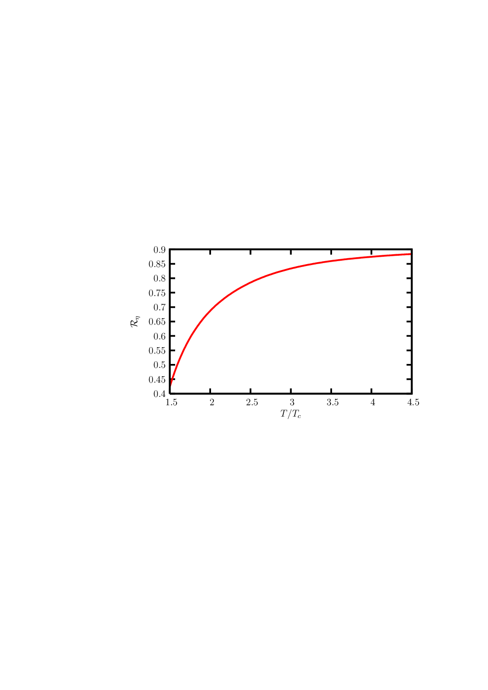
Let us consider the ratio to see how for LEOS deviates from its ideal counterpart. This ratio is model independent to the extent that it does not depend on . In making this statement it is understood that as a phenomenological parameter, is not sensitive to the EOS employed [44, 45]. The behavior of as a function of is shown in Fig.7, from which it is clear that the inclusion of interactions significantly decreases the shear viscosity. As expected, the ratio asymptotically approaches unity. Therefore, the shear viscosity serves as a good diagnostic to distinguish the EOS at RHIC.
To see the extent to which the interactions effect the , we consider the ratio . The behavior of as a function of temperature is shown in Fig.8. From Fig.8 it is easy to see that interactions coming from LEOS decrease the ratio by 35% near and near . It approaches the corresponding ideal value only asymptotically. This crucial observation reinforces the necessity of employing realistic equations of state, in particular LEOS for determining the transport properties of the plasma. Our findings lead to an interesting conclusion that both and the ratio, are good diagnostics as far as the effects of interactions are concerned.

5 Conclusion and Outlook
In conclusion, we have developed a quasi-particle model in the spirit of Landau’s Fermi liquid theory to extract the distribution function for gluons from pure gauge theory equation of state. We find that the description is exact. We show that all the interaction effects can be captured in the effective fugacity for gluons. We have determined the new dispersion relation for quasi-gluons which brings out the effect of trace anomaly and also the collective nature of these excitations. We have determined the temperature dependence of the Debye mass which can be exactly matched with the lattice parametrized Debye mass by defining the effective gluon charge in terms of the QCD running coupling constant. Employing the quasi-particle model, we have determined and the ratio . In doing this, we have determined as function of temperature for LEOS. We have also determined the temperature dependence of gluon quenching parameter. We find that both and for LEOS decrease significantly as compare to the ideal EOS. We find that there is a possible violation of AdS/CFT bound for for lattice equation of state. It would be of interest to extend this analysis to the full QCD EOS and also to study the bulk viscosity. Should the quasi-particle model work for full QCD equally well, it opens up interesting possibilities of building effective theories.
Acknowledgment: We are thankful to Frithjof Karsch for providing us with the lattice data which made this analysis possible. VC acknowledges Saumen Datta for useful discussions and Ashok Garai for help in the numerical part. He acknowledges the Raman Research Institute, Banglore (India) for hospitality where part of this work was completed, and C.S.I.R, New Delhi (India) for financial support.
6 Appendix
In this appendix, we show how one determines the anisotropy parameter, for LEOS. We start with the equilibrium distribution function , where is purely temperature dependent, for the quasi-gluons. The action of the drift operator on is given by
| (34) | |||||
where we recognize that , is the modified dispersion relation. In the local rest frame of the fluid, this expression is formally the same as Eq.(6.1) in [15] where of course . Similarly, the expressions for the Debye mass and the continuity equation for the energy momentum tensor ( Eqs.(6.3)-(6.7) in [15]) also undergo the same modification via the new dispersion relation.
The final expression for the drift term after imposing the energy-momentum conservation is obtained as
where is the speed of sound. The third term in Eq.(6) will contribute to the bulk viscosity. To determine the bulk viscosity for LEOS, we need to include trace part in the ansatz for [15]. In this case, the form of the perturbation, gets modified as,
| (36) |
The second term in the above expression will generate a term proportional to in the force term, and the comaprison of this term with the third term in Eq.(6) would lead to the expression for and hence the bulk viscosity. Since we are only interested in the shear viscosity here, we concentrate on the form of .
On the other hand, the force term will have exactly the same mathematical form as in [15](Eq.(6.13)), if we consider only the traceless part of velocity gradient in the expression for . The same mathematical structure of the Force term in this case follows from the isotropy of . The force term in the case of a purely chromomagnetic plasma in the present case will be,
| (37) | |||||
On comparing of the Force term and the first term in the RHS of Eq.(6), we infer that the anisotropy parameter is given by
| (38) |
References
- (1) Kenneth G. Wilson, Phys. Rev. D 10, 2445 (1974).
- (2) Landau, Lifshitz. Vol. 9. Statistical physics part 2 (Pergamon, 1980).
- (3) Vinod Chandra, Ravindra Kumar, V. Ravishankar, Phys. Rev. C 76, 054909(2007).
- (4) Vinod Chandra, Akhilesh Ranjan, V. Ravishankar, Euro. Phys. J A 40, 109 (2009); arXiv:0801.1286(hep-ph).
- (5) Vinod Chandra and V. Ravishankar, Euro. Phys. J C 59, 705 (2009) (arXiv:0805.4820(nucl-th)).
- (6) STAR Collaboration (John Adams et al.), Nucl.Phys. A 757, 102 (2005); PHENIX Collaboration (K. Adcox et al.), Nucl.Phys. A 757, 184, (2005); B.B. Back et al., Nucl.Phys. A757, 28 (2005).
- (7) Hans-Joachim Drescher, Adrian Dumitru, Clement Gombeaud, Jean-Yves Ollitrault, Phys. Rev. C 76, 024905 (2007).
- (8) Edward Shuryak, Nucl.Phys. A 774, 387 (2006).
- (9) P.Kovtun, D.T.Son, A.O.Starinets, Phys. Rev. Lett. 94, 111601 (2005).
- (10) Boyd et al., Nucl. Phys. B 469, 419 (1996); Phys. Rev. Lett. 75, 4169 (1995).
- (11) Frithjof Karsch, Lect. Notes Phys. 583, 209 (2002).
- (12) Rajiv V. Gavai, Pramana 67, 885 (2006) (hep-ph/0607050.)
- (13) M. Cheng et al., Phys. Rev. D 77, 014511 (2008) (arXiv:0710.0354).
- (14) Peter Arnold, Guy D. Moore, Laurence G. Yaffe, JHEP 0011, 001 (2000); JHEP 0305, 051 (2003).
- (15) M. Asakawa, S.A. Bass, B. Müller, Phys. Rev. Lett. 96, 252301 (2006); Prog. Theor. Phys. 116, 725 (2007).
- (16) Zhe Xu, Carsten Greiner, Phys. Rev. Lett. 100, 172301 (2008).
- (17) Dmitri Kharzeev and Kirill Tuchin, JHEP 09, 093 (2008).
- (18) F. Karsch, D. Kharzeev and K. Tuchin, Phys. Lett. B 663, 217 (2008) (arXiv:0711.0914).
- (19) Peshier et al., Phys. Lett. B 337, 235 (1994)
- (20) Peshier et al., Phys. Rev. D 54, 2399 (1996); Phys.Rev. C 61, 045203 (2000), Phys. Rev. D 66, 094003 (2002).
- (21) Allton et al., Phys. Rev. D 68, 014507 (2003); Phys.Rev. D 71, 054508 (2005).
- (22) P. Castorina, M. Mannarelli, Phys. Rev. C 76, 054901 (2001)(hep-ph/0701206); Phys. Lett. B 644, 336 (2007)(hep-ph/0510349).
- (23) Mingzhe Li, Haixiang Fu, Zhipeng Zhang and Jican Chen, Phys. Rev. A 75, 045602 (2007).
- (24) Ji-sheng Chen, Jia-rong Li, Yan-ping Wang and Xiang-jun Xia, arXiv:0712.0205(cond-mat).
- (25) T. Haugerud, T. Haugset, F. Ravndal, arXiv:cond-mat/9605100.
- (26) Tor Haugset, Hårek Haugerud nd Jens O. Andersen, Phys. Rev. A 55, 2922 (1997).
- (27) Jae Dong Noh, G. M. Shim and Hoyun Lee, Phys. Rev. Lett. 94, 198701 (2005).
- (28) Klaus Kristen, David J. Toms, Physics Letters A 243, 137 (1998).
- (29) P.F. Kelly, Q. Liu, C. Lucchesi, C. Manuel, Phys.Rev.Lett. 72, 3461 (1994); D. F. Litim and C. manual, Phys.Rept. 364, 451 (2002); Jean-Paul Blaizot, Edmond Iancu, Phys.Rept. 359, 355 (2002); Phys.Rev.Lett. 70, 3376 (1993).
- (30) Akhilesh Ranjan and V. Ravishankar, arXiv:0707.3697.
- (31) Agnes Mocsy and Peter Petreczky, Phys. Rev. Lett. 99, 211602 (2007).
- (32) S. Jacobs, M. G. Olsson and C. Suchyta, Phys. Rev. D 33, 3338 (1986).
- (33) O. Kaczmarek, F. Karsch, P. Petreczky, F. Zantow, Phys.Lett. B543, 41 (2002); Phys. Rev. D70, 074505 (2004); Olaf Kaczmarek, Felix Zantow, Phys.Rev. D71, 114510 (2005).
- (34) M. Laine, Y. Schroder, JHEP 0503, 067 (2005).
- (35) A. Majumder, B. Müller, X.-N. Wang, Phys. Rev. Lett. 99, 192301 (2007).
- (36) Helmut Satz, Nucl.Phys. A 783, 249 (2007) (arXiv:hep-ph/0609197).
- (37) W.M. Alberico, A. Beraudo, A. De Pace, A. Molinari, Phys. Rev. D 75, 074009(2007).
- (38) S. Datta, et al., Phys. Rev.D 69, 094507 (2004).
- (39) Gert Aarts, Chris Allton, Mehmet Bugrahan Oktay, Mike Peardon, Jon-Ivar Skullerud, Phys. Rev. D 76, 094513 (2007).
- (40) T. Umeda et al., Eur. Phys. J. C 39S1, 9 (2005) (arXiv:hep-lat/0211003).
- (41) Vineet Agotiya, Vinod Chandra, Binoy K. Patra, arXiv:0808.2699 (to appear in Phys. Rev. C).
- (42) E M Lifshitz and L P Pitaevskii, Physical Kinetics(Landau and Lifshitz; Volume 10) Pergamon Press.
- (43) T. H. Dupree, Phys. Fluids 9, 1773 (1966), Phys. Fluids 11; 2680 (1968).
- (44) Hanzhong Zhang, J. F. Owens, Enke Wang, Xin-Nian Wang, Phys. Rev. Lett. 98, 212301 (2007); A. Majumder, C. Nonaka, S. A. Bass, arXiv:nucl-th/0703019.
- (45) R.Baier, Yu.L.Dokshitzer, A.H.Mueller, S.Peigné, D.Schiff, Nucl.Phys. B 483,291 (1997); N. Armesto, L. Cunqueiro, C. A. Salgado, W.-C. Xiang, arXiv:0710.3073.
- (46) R. Baier and P. Romatschke, arXiv:nucl-th/0610108.
- (47) H. B. Meyer, Phys. Rev. D 76, 10171 (2007)(arXiv:0704.1801(hep-lat).
- (48) A. Nakamura and Sunao Sakai, Phys. Rev. Lett. 94, 072305 (2005).
- (49) Lacey et al, Phys. Rev. Lett. 98, 092301 (2007).
- (50) Zhe Xu and Carsten Greiner, Phys. Rev. Lett. 100, 172301 (2008).
- (51) Adare et al, Phys. Rev. Lett. 98, 172301 (2007).
- (52) Sean Gavin and Mohamed Abdel-Aziz, Phys. Rev. Lett. 97, 162302 (2006).
- (53) Zhe Xu, Carsten Greiner, Horst Stoecker, Phys. Rev. Lett. 101, 082302 (2008).