In this section, we will consider a surface operator ${\cal{O}}_{\Sigma}$ of $SU(N)$ ${\cal{N}}=4$ super Yang-Mills theory on $\mathbb{R}^{4}$ with coordinates $(x^{0},x^{1},x^{2},x^{3})$, or on $\mathbb{C}^{2}$ with coordinates $(z^{1},z^{2})$. Our conventions for the gauge theory are collected in appendix A.

As in [1], we characterize a surface operator by the boundary condition of bosonic fields near codimension 2 singularities. Semi-classically the surface operator is given by a classical solution with these boundary conditions and its quantum fluctuations. Likewise, any classical solution with a codimension 2 singularity corresponds to a surface operator, defined by the boundary conditions near the singularity of the classical solution.

In this paper we focus on the classical solutions in which the gauge fields are flat; in a suitable gauge choice we can set $A_{\mu}=0$ at least locally. The non-trivial field excitations in the classical solution are the scalar fields. In the 1/2 BPS case [1, 9] the solution with simple pole

is considered. The higher order poles can also be considered [11]. Then what happens when the singularity has branches? That is what we address in this paper.

In order to explain our basic idea and make things explicit, we focus in this section and next on the classical solution of the type

We will consider more generic classical solutions in section 4. In particular, other examples of the 1/4 BPS surface operators are found in section 4.3.2. In eq.(2.2) we include both $z^{1}$ and $z^{2}$ in order to preserve the dilatation symmetry. This dilatation symmetry is useful for Wick rotation as we will explain later. This configuration is singular along the two planes with $z^{1}=0$ as well as $z^{2}=0$. Hence when we consider the surface operator by the path integral, we impose the boundary condition at both $z^{1}=0$ and $z^{2}=0$.

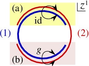
The behavior of the scalar field (2.2) does not look like a consistent configuration because it is not single valued²² 2 Similar double valued configuration also appears in the conformal vortex loop operator in 3-dimensional super-conformal Chern-Simons theory[18].. However we can make it a consistent configuration by introducing the gauge field holonomy as follows. We consider the scalar $\Phi$, which is an $N\times N$ matrix, and the gauge fields

where $\beta$ is a real positive parameter. These fields are not single valued. For example, the value of the scalar field has $\mathbb{Z}_{2}$ monodromy when $z^{1}$ goes to $z^{1}e^{2\pi i}$. This monodromy can be cancelled by the gauge holonomy. Let us introduce two patches of coordinates ($z^{1}=r_{1}e^{i\phi_{1}}$) in order to explain this holonomy (see figure 1).

1. (1)

   $0<\phi_{1}<2\pi$ (branch cut at $\phi_{1}=\pi$).

2. (2)

   $-\pi<\phi_{1}<\pi$ (branch cut at $\phi_{1}=0$).

The intersection of these two patches is two disconnected regions: (a) $0<\phi_{1}<\pi$ and (b) $-\pi<\phi_{1}<0$. The gauge transformation between these two patches is chosen as follows. In the region (a), (1) and (2) are trivially identified, namely $\Phi^{(1)}=\Phi^{(2)},\ A_{\mu}^{(1)}=A_{\mu}^{(2)}$. On the other hand, in the region (b) they are related by the gauge transformation with the constant parameter $g\in$SU($N$) defined as

The fields are transformed under the transformation as,

The eq.(2.5) are consistent with $A^{(1)}_{\mu}=A^{(2)}_{\mu}=0$ because $g$ is a constant. Moreover the monodromy due to the square root branch can be canceled by this gauge transformation.

Note that the configuration (2.3) satisfies the equation of motion.

We can introduce further gauge holonomy which commute with $\Phi$ and $g$. The field configuration (2.3) and the holonomy (2.4) break the gauge symmetry SU$(N)$ to U$(1)\times$SU$(N-2)$. Therefore we can introduce extra holonomy included in this U$(1)$. In other words, we can change the gauge transformation (2.4) to $g_{\alpha_{1}}$ which includes parameter $\alpha_{1}$ as

This parameter $\alpha_{1}$ is an analogue of the parameter $\alpha$ in [1]. There is also a monodromy around $z^{2}=0$, and the holonomy $g_{\alpha_{2}}$ is introduced to cancel this monodromy. These two parameters $(\alpha_{1},\alpha_{2})$ fix the holonomy globally³³ 3 This is so simple in this special example because the monodromy group is abelian. It is also worth to note that the fundamental group of the space, obtained by removing two planes $z^{1}=0$ and $z^{2}=0$ from $\mathbb{C}^{2}$, is an abelian group $\mathbb{Z}\times\mathbb{Z}$. In the more general case, the problem seems to be more involved..

We can also introduce the two dimensional theta angle as the similar way as in [1] by inserting the operator

where $F|_{{\rm U}(1)}$ are the unbroken U$(1)$ part of the field strength. There are also similar parameter $\eta_{2}$ at $z^{2}=0$.

We can also introduce the parameter $\gamma$ as in [1], by making $\beta$ complex valued. However, to avoid undue complications, we choose $\beta$ as a real positive number. The phase can be restored to nontrivial value at any stage of our discussion.

Instead of introducing two patches and a gauge transformation between them, we can choose the gauge field $A$ to be nontrivial, $A=-\frac{i}{2\pi}\sum_{i=1,2}\ln g_{\alpha_{i}}d\phi_{i}$. In this frame, the scalar field takes the form

and there is no monodromy. However we will not use this frame in the rest of this paper since this frame is not convenient to see the supersymmetry.

Let us consider how to do the path-integral around this multi-valued configuration. In string theory, a similar situation occurs when one consider the twisted sector of strings in the presence of orbifolds. The boundary condition of the fluctuation $\delta\Phi$ can be chosen by the following

where $\Phi$ is given in (2.3), a solution of the equation of motion. Expand $\delta\Phi$ as

where $T_{A}$ are the basis of the $N\times N$ matrix, which diagonalize the adjoint $g_{\alpha_{i}}$ action, namely $g_{\alpha_{i}}T^{A}g_{\alpha_{i}}^{-1}=\exp(2\pi i\xi_{i}(A))T^{A}$ with some numbers $\xi_{i}(A)$. $\delta\Phi^{A}$ can be expanded to the Fourier series as $\delta\Phi^{A}=\sum_{n_{1},n_{2}\in\mathbb{Z}}\exp[i\sum_{i}(n_{i}+\xi_{i}(A))\phi_{i}]h^{A}_{n_{1},n_{2}}$ and the measure of the path-integral can be written as $D\delta\Phi=\prod_{A,n_{1},n_{2}}Dh^{A}_{n_{1},n_{2}}$. The other fields are also treated as the same way.

The configuration (2.3) preserves the dilatation symmetry. This dilatation symmetry acts on the scalar field with a real positive parameter $\alpha$ as

Under the dilatation symmetry, the configuration (2.3) is invariant, i.e. $\Phi^{\prime}(z_{1},z_{2})=\Phi(z_{1},z_{2})$. The dilatation symmetry is useful to write an analogous configuration in Lorentzian signature. By a Weyl transformation, flat Euclidean space $\mathbb{R}^{4}$ can be mapped into $\mathbb{R}\times S^{3}$. Dilatation transformations in $\mathbb{R}^{4}$ are mapped to time translations in $\mathbb{R}\times S^{3}$, so in this frame, the configuration (2.3) is time independent. Thus we can safely perform the Wick rotation of $\mathbb{R}$ direction and get a static configuration of ${\cal{N}}=4$ SYM in $\mathbb{R}_{\rm time}\times S^{3}$. This fact is useful to find a gravity counterpart in Lorentzian global $AdS_{5}\times S^{5}$.

The surface operator defined in (2.3) preserves 1/4 of the supersymmetry and the super-conformal symmetry. To see this, we need to consider the variation of the fermion $\psi$ of ${\cal{N}}=4$ SYM, given in (A.4). For the background field as in (2.3), the variation can be written conveniently if we use the complex coordinates:

where $\bar{\Phi}$ is the hermitian conjugation of $\Phi$. $\epsilon(z)$ combines the parameters of super-Poincaré transformations $\epsilon_{0}$ and of super-conformal transformations $\epsilon_{1}$, each of which is a 16 component spinor, as follows

The variation of the fermion (2.10) vanishes, if we impose the following condition on $\epsilon_{i}$,

or equivalently

In the derivation of this condition, we use the relation

which holds because $\Phi$ is a degree $(-1)$ homogeneous function of $z^{1},z^{2}$.

The bosonic unbroken symmetries for the quarter BPS surface operator (2.3) are as follows. The surface operator in consideration (2.3) preserves the dilatation symmetry $\mathbb{R}_{+}$ of the 4-dimensional Euclidean conformal symmetry SO$(1,5)$. It is also invariant under an $SO(4)$ subgroup of the R-symmetry SO$(6)$. It breaks spacetime rotational symmetry, while it preserves SO$(2)_{a}$, and SO$(2)_{b}$ symmetry which are the combinations of the spacetime rotation and R-rotation; SO$(2)_{a}$ is the diagonal part of SO$(2)_{R}\times$SO$(2)_{01}\times$SO$(2)_{23}$, while SO$(2)_{b}$ is the difference of SO$(2)_{01}$ and SO$(2)_{23}$. The super charge in the $({\bf 4},{\bf 4})$ representation of SO$(4,2)\times$SO$(6)$ is reduced to $({\bf 2},1)$ and $(1,{\bf 2})$ of the SU$(2)\times$SU$(2)\sim$SO$(4)$.

In this section, we will consider the expectation value of the quarter BPS surface operator, ${\cal{O}}_{\Sigma}$, defined in (2.3). We expect this expectation value to be $1$ due to the supersymmetry. The expectation value is defined as the path integral with the boundary condition at the singularity. This path integral is approximated by the classical SYM action:

The relevant part of ${\cal{N}}=4$ SYM action in (A.1) is

In the presence of the surface operator as in (2.3), it leads to the following:

Let us use the polar coordinate, $z^{i}=r_{i}e^{i\phi_{i}}$ and regulate $r_{i}\in(r_{0},\infty)$ for $i=1,2$ . Then

Our conventions for the measure are given in (A.5). As in [10], we add a boundary term to impose the appropriate boundary condition. Without additional boundary terms, the variation of the action gives

This surface term would impose the boundary conditions $r_{1}\partial\Phi/\partial r_{1}=0$ at $r_{1}=r_{0}$ and $r_{2}\partial\Phi/\partial r_{2}=0$ at $r_{2}=r_{0}$, which are not satisfied by the solution (2.3). In order to get rid of this additional condition, we add the following boundary term to the action.

Adding this boundary term makes the boundary conditions $2r_{1}\partial\Phi/\partial r_{1}+\Phi=0$ at $r_{1}=r_{0}$ and $2r_{2}\partial\Phi/\partial r_{2}+\Phi=0$ at $r_{2}=r_{0}$, which are actually satisfied by the solution (2.3).

The total action is summed up to be zero, $(S+S_{b})|_{\Sigma}=0$, thus

As considered in [19, 20, 21, 22, 23], the surface operator may have conformal anomalies since the surface operator is defined on an even dimensional submanifold. To compute the anomaly, we need to evaluate the action of a surface operator defined on $\Sigma$ with non-trivial curvature or Weyl tensor. This will be an interesting future work.

The correlation function of a local operator ${\cal{O}}(\zeta)$ inserted at the point $z^{m}=\zeta^{m}$ and the surface operator ${\cal{O}}_{\Sigma}$ in the semi-classical limit is given by the classical value of the operator in the classical solution.

The correlation function of the surface operator (2.3) and a chiral primary operators is non-trivial when the CPO is invariant under $SO(4)$ subgroup of $SO(6)$ R-symmetry. We use the notation of the $SO(4)$ invariant CPO as given in [24, 10]

$\Delta$ is the conformal dimension. $k$ is the charge under $SO(2)$ of $SO(2)\times SO(4)$ subgroup of R-symmetry, $k=-\Delta,-\Delta+2,\cdots,\Delta$. We give the definition of $C^{i_{1},\cdots,i_{\Delta}}$ in (E.2) and review the relevant aspects of the spherical harmonics in appendix E.1. The relevant part for the correlation function with the surface operator in (2.3),

where $C_{\Delta,k}$ is given in (E.3), and $[\cdot]_{\text{sym}}$ means all the products inside are totally symmetrized. Using $\Phi_{2}=\Phi_{3}=0$ the correlation function evaluated by (2.17) is

Note that the correlation function vanishes for odd $\Delta$, since the two diagonal components inside the trace have the opposite sign.

The correlation function of the ${\cal{O}}_{\Sigma}$ in (2.3) with a Wilson line or the stress-energy tensor can be interesting physical quantities to investigate, as for the half BPS surface operator in [10]. However we will not pursue the issue here.

Let us now consider the holographic dual of the surface operator defined in (2.3). The following complex coordinate system for $AdS_{5}\times S^{5}$ is convenient for this purpose:

We can relate it to the global coordinates of $AdS_{5}\times S^{5}$ as follows:

Then the metric (3.1) becomes

where $d\Omega_{3}^{2}$ and $d\Omega_{5}^{2}$ are the metrics of the unit $S^{3}$ and the unit $S^{5}$ expressed as

To be supersymmetric, we have the following 5 form field strength in the background:

In this paper we choose the unit of length such that the radius of $AdS_{5}$ is $1$, namely $4\pi g_{s}N\alpha^{\prime 2}=1$. In these units $\alpha^{\prime}=1/\sqrt{\lambda}=1/\sqrt{4\pi g_{s}N}$, and the D3-brane tension $T_{D3}$ is expressed as

We propose that a probe D3-brane, wrapping a 4 dimensional subspace $\Sigma_{4}$ defined by the following holomorphic equations ,

is dual to the surface operator in (2.3). Here $\kappa$ is a parameter related to $\beta$. The precise relation between $\beta$ and $\kappa$ are determined later in eq.(3.29), according to the correlation function with the chiral primary operators.

The parameters $(\alpha_{1},\alpha_{2},\eta_{1},\eta_{2})$ are mapped to the gauge field $A$ on the D3-brane and its magnetic dual $\tilde{A}$ as

Note that the configuration (3.5) is $\tau$ independent, i.e. static. Thus we can Wick rotate the configuration easily by replacing $\tau=it$ and consider the same static configuration in the Lorentzian signature. It is convenient to consider the Lorentzian signature especially when checking the supersymmetry, which we do in the next subsection.

To check the preserved supersymmetry of the probe D-brane, we can use the kappa symmetry projection [25, 26, 27, 28, 29, 30, 5]. To this end, it is advantageous to use a 12 dimensional embedding space $\mathbb{C}^{1,2}\times\mathbb{C}^{3}$ with coordinates $(Z^{0},Z^{1},Z^{2},W^{1},W^{2},W^{3})$, as in [31, 32]. The reason is that the Killing spinor of the embedding space is constant Dirac spinor with 64 complex components, while the Killing spinor of the physical space depends on the space-time. We can get the 10 dimensional physical space $AdS_{5}\times S^{5}$ using the constraints:

Reduction of the constant Killing spinor in the embedding space to the one in the physical space is done by the following conditions,

where $\gamma^{A}$ are defined in (C.1).

We review the relevant aspects of the kappa symmetry projection and the conventions for the embedding space in appendix B and appendix C. General discussions about super-symmetric branes in $AdS_{5}\times S^{5}$ can be found in [5].

We can use an embedding map as follows:

The D3-brane worldvolume $\Sigma_{4}$ defined by (3.5) is an intersection of the physical space and a six dimensional holomorphic space $\Sigma_{6}$ in the embedding space defined by:

Note that we can let eq.(3.10) be the same form of eq.(3.5) due to our embedding map (3.9).

Two vectors $E_{r_{1}},E_{r_{2}}$ in $T\Sigma_{6}\backslash T\Sigma_{4}$ are projections of the two normal vectors of $AdS_{5}\times S^{5}$ in the embedding space on the $T\Sigma_{6}$. One of these vectors is time-like and the other is space-like. We will use $r_{1}$ as a time-like direction.

Since $T\Sigma_{6}$ is closed under a complex structure $I$, given as $I\cdot{\frac{\partial}{\partial Z^{A}}}=i\frac{\partial}{\partial Z^{A}}$ and $I\cdot\frac{\partial}{\partial\bar{Z}^{\bar{A}}}=-i\frac{\partial}{\partial\bar{Z}^{\bar{A}}}$ , $I\cdot E_{r_{i}}$ are in $T\Sigma_{4}$ . We call these vectors $E_{0},E_{1}$. We can linearly combine $E_{0},E_{1}$ to form null vectors $E_{\pm}$ . There leave two linearly independent vectors in $T\Sigma_{4}$, which are orthogonal to $E_{\pm}$ and closed under $I$. The holomorphic/anti-holomorphic part of these vectors are defined to be $E_{z},E_{\bar{z}}$. From the construction, the followings hold:

We normalize the vectors as:

Using eqs.(3.11),(3.12), the projection operator (B.1) along the D3-brane can be written in the following form:

As shown in [31], the condition for the preserved supersymmetry of a D3-brane in the embedding space becomes

where $\Gamma$ is the projection operator along the D3-brane, for our case (3.13).

Let us now consider the holographic dual of the surface operator in (2.3). We will use $(Z^{3},Z^{4},Z^{5})\equiv(W^{1},W^{2},W^{3})$. For the holomorphic space $\Sigma_{6}$ defined by (3.10), the tangent vectors are $v_{0}\equiv Z^{0}\partial_{0}$, $v_{1}\equiv\left(Z^{1}\partial_{1}+Z^{2}\partial_{2}-Z^{3}\partial_{3}\right)$, $v_{2}\equiv\left(Z^{1}\partial_{1}-Z^{2}\partial_{2}\right)$ and their complex conjugates. The vector in $T\left(\mathbb{C}^{1,2}\times\mathbb{C}^{1}\right)\backslash T\Sigma_{6}$ is $v^{\perp}\equiv\frac{1}{2}\bar{Z}^{3}\bar{Z}^{2}\partial_{1}+\frac{1}{2}\bar{Z}^{3}\bar{Z}^{1}\partial_{2}+\bar{Z}^{1}\bar{Z}^{2}\partial_{3}$. To project the normal vectors of $AdS_{5}\times S^{5}$ on $T\Sigma_{6}$, we note that on $\Sigma_{6}$,

where $\nu\equiv 4|Z^{1}Z^{2}|^{2}+|Z^{1}|^{2}+|Z^{2}|^{2}$. We project out $v^{\perp}$ then linearly recombine the result to get a convenient form of $E_{r_{1}},E_{r_{2}}$. We choose

We can now construct tangent vectors satisfying (3.11), (3.12) as follows:

From the construction, $E_{\pm}^{A}\gamma_{A}=\frac{i}{2}(\pm E_{r_{1}}^{A}+E_{r_{2}}^{A})\gamma_{A},E_{\pm}^{\bar{A}}\gamma_{\bar{A}}=-\frac{i}{2}(\pm E_{r_{1}}^{\bar{A}}+E_{r_{2}}^{\bar{A}})\gamma_{\bar{A}}$. Due to the orthogonality of $E_{r_{1}}$ and $E_{r_{2}}$ , the relations $\{E_{r_{1}}^{A}\gamma_{A},E_{r_{2}}^{\bar{B}}\gamma_{\bar{B}}\}=\{E_{r_{1}}^{\bar{A}}\gamma_{\bar{A}},E_{r_{2}}^{B}\gamma_{B}\}=0$ hold. $\Gamma^{r_{1}}$ is given as $\Gamma^{r_{1}}=-\Gamma_{r_{1}}=-(E_{r_{1}}^{A}\gamma_{A}+E_{r_{2}}^{\bar{B}}\gamma_{\bar{B}})$. Using these, the projection (3.14) can be written as

Let us impose the following conditions on the Killing spinor $\epsilon$,

It implies that $\gamma_{1\bar{2}}\epsilon=\gamma_{1\bar{3}}\epsilon=\gamma_{2\bar{3}}\epsilon=0$, since $\gamma_{1\bar{2}}\gamma_{1\bar{1}}=-\gamma_{1\bar{2}}\gamma_{2\bar{2}}=-\frac{1}{2}\gamma_{1\bar{2}}$ , etc. It also implies that $\gamma_{0\bar{0}}\epsilon=\frac{1}{2}\epsilon,\gamma_{\bar{0}}\epsilon=0,$ when combined with the reduction of the spinor (3.8). Under the imposition (3.16), the right hand side of (3.15) is reduced to $i\epsilon$, being equivalent to the condition in (3.14). It shows that the probe D-brane preserves 1/4 of the supersymmetry.

Our construction can be regarded as a special case of [32], in which a holomorphic space defined by three holomorphic homogeneous functions $f_{k}(Z^{0},Z^{1},Z^{2},W^{1},W^{2},W^{3})$ for $k=1,2,3$, when $Z^{i},W^{i}$ are assigned weights $+1,-1$, has been considered. The probe D3-brane wrapping this holomorphic space has been shown to preserve 1/16 of supersymmetry. In our case, the $\frac{\partial}{\partial t}$ vector in $AdS$ space is tangential to the D-brane, thus the transverse velocity $v$ vanishes.

At the semi-classical level, we evaluate the expectation value of a surface operator by

where $S_{D3}$ is on-shell action of the probe D3-brane corresponding to the surface operator. This holds in the large $N$ limit ($N\gg 1$) and the large t’Hooft coupling limit,

The action of the D3-brane can be expressed in terms of of $DBI$ action and Wess-Zumino term,

$\xi^{m}$ are the world-volume coordinates, and $G_{mn}$ is the induced metric on the world-volume. $C_{4}$ is the R-R four form of which field strength is given is (3.3). $T_{D3}$ is the tension of the D3-brane (see eq.(3.4)).

Let us consider the probe D3-brane wrapping $\Sigma_{4}$ defined by (3.5). We will use complex coordinates in $AdS_{5}\times S^{1}$ with the metric ⁴⁴ 4 The other directions in $S^{5}$ are irrelevant to our discussion in this subsection :

We choose the gauge of the R-R four form as

We sometimes use polar coordinates $r_{i}e^{i\phi_{i}}=z^{i}$, $\omega=y^{-1}e^{i\theta}$. $\theta$ is the angle of $S^{1}$ in $S^{5}$. The definition of $y$ is to restore the Poincaré metric of $AdS_{5}$ as

References

- [1] S. Gukov and E. Witten, “Gauge theory, ramification, and the geometric langlands program,” arXiv:hep-th/0612073.
- [2] J. M. Maldacena, “The large N limit of superconformal field theories and supergravity,” Adv. Theor. Math. Phys. 2 (1998) 231–252, arXiv:hep-th/9711200.
- [3] S. S. Gubser, I. R. Klebanov, and A. M. Polyakov, “Gauge theory correlators from non-critical string theory,” Phys. Lett. B428 (1998) 105–114, arXiv:hep-th/9802109.
- [4] E. Witten, “Anti-de Sitter space and holography,” Adv. Theor. Math. Phys. 2 (1998) 253–291, arXiv:hep-th/9802150.
- [5] K. Skenderis and M. Taylor, “Branes in AdS and pp-wave spacetimes,” JHEP 06 (2002) 025, arXiv:hep-th/0204054.
- [6] N. R. Constable, J. Erdmenger, Z. Guralnik, and I. Kirsch, “Intersecting D3-branes and holography,” Phys. Rev. D68 (2003) 106007, arXiv:hep-th/0211222.
- [7] H. Lin, O. Lunin, and J. M. Maldacena, “Bubbling AdS space and 1/2 BPS geometries,” JHEP 10 (2004) 025, arXiv:hep-th/0409174.
- [8] H. Lin and J. M. Maldacena, “Fivebranes from gauge theory,” Phys. Rev. D74 (2006) 084014, arXiv:hep-th/0509235.
- [9] J. Gomis and S. Matsuura, “Bubbling surface operators and S-duality,” JHEP 06 (2007) 025, arXiv:0704.1657 [hep-th].
- [10] N. Drukker, J. Gomis, and S. Matsuura, “Probing N=4 SYM With Surface Operators,” JHEP 10 (2008) 048, arXiv:0805.4199 [hep-th].
- [11] E. Witten, “Gauge Theory And Wild Ramification,” arXiv:0710.0631 [hep-th].
- [12] S. Gukov and E. Witten, “Rigid Surface Operators,” arXiv:0804.1561 [hep-th].
- [13] J. A. Harvey and A. B. Royston, “Localized Modes at a D-brane–O-plane Intersection and Heterotic Alice Strings,” JHEP 04 (2008) 018, arXiv:0709.1482 [hep-th].
- [14] E. I. Buchbinder, J. Gomis, and F. Passerini, “Holographic Gauge Theories in Background Fields and Surface Operators,” JHEP 12 (2007) 101, arXiv:0710.5170 [hep-th].
- [15] J. A. Harvey and A. B. Royston, “Gauge/Gravity duality with a chiral N=(0,8) string defect,” JHEP 08 (2008) 006, arXiv:0804.2854 [hep-th].
- [16] D. Serban and M. Staudacher, “Planar N = 4 gauge theory and the Inozemtsev long range spin chain,” JHEP 06 (2004) 001, arXiv:hep-th/0401057.
- [17] D. E. Berenstein, J. M. Maldacena, and H. S. Nastase, “Strings in flat space and pp waves from N = 4 super Yang Mills,” JHEP 04 (2002) 013, arXiv:hep-th/0202021.
- [18] N. Drukker, J. Gomis, and D. Young, “Vortex Loop Operators, M2-branes and Holography,” arXiv:0810.4344 [hep-th].
- [19] D. E. Berenstein, R. Corrado, W. Fischler, and J. M. Maldacena, “The operator product expansion for Wilson loops and surfaces in the large N limit,” Phys. Rev. D59 (1999) 105023, arXiv:hep-th/9809188.
- [20] C. R. Graham and E. Witten, “Conformal anomaly of submanifold observables in AdS/CFT correspondence,” Nucl. Phys. B546 (1999) 52–64, arXiv:hep-th/9901021.
- [21] M. Henningson and K. Skenderis, “Weyl anomaly for Wilson surfaces,” JHEP 06 (1999) 012, arXiv:hep-th/9905163.
- [22] A. Gustavsson, “On the Weyl anomaly of Wilson surfaces,” JHEP 12 (2003) 059, arXiv:hep-th/0310037.
- [23] A. Gustavsson, “Conformal anomaly of Wilson surface observables: A field theoretical computation,” JHEP 07 (2004) 074, arXiv:hep-th/0404150.
- [24] K. Skenderis and M. Taylor, “Anatomy of bubbling solutions,” JHEP 09 (2007) 019, arXiv:0706.0216 [hep-th].
- [25] M. Cederwall, A. von Gussich, B. E. W. Nilsson, and A. Westerberg, “The Dirichlet super-three-brane in ten-dimensional type IIB supergravity,” Nucl. Phys. B490 (1997) 163–178, arXiv:hep-th/9610148.
- [26] M. Aganagic, C. Popescu, and J. H. Schwarz, “D-brane actions with local kappa symmetry,” Phys. Lett. B393 (1997) 311–315, arXiv:hep-th/9610249.
- [27] M. Cederwall, A. von Gussich, B. E. W. Nilsson, P. Sundell, and A. Westerberg, “The Dirichlet super-p-branes in ten-dimensional type IIA and IIB supergravity,” Nucl. Phys. B490 (1997) 179–201, arXiv:hep-th/9611159.
- [28] E. Bergshoeff and P. K. Townsend, “Super D-branes,” Nucl. Phys. B490 (1997) 145–162, arXiv:hep-th/9611173.
- [29] M. Aganagic, C. Popescu, and J. H. Schwarz, “Gauge-invariant and gauge-fixed D-brane actions,” Nucl. Phys. B495 (1997) 99–126, arXiv:hep-th/9612080.
- [30] E. Bergshoeff, R. Kallosh, T. Ortin, and G. Papadopoulos, “kappa-symmetry, supersymmetry and intersecting branes,” Nucl. Phys. B502 (1997) 149–169, arXiv:hep-th/9705040.
- [31] A. Mikhailov, “Giant gravitons from holomorphic surfaces,” JHEP 11 (2000) 027, arXiv:hep-th/0010206.
- [32] S. Kim and K.-M. Lee, “1/16-BPS black holes and giant gravitons in the space,” JHEP 12 (2006) 077, arXiv:hep-th/0607085.
- [33] H. J. Kim, L. J. Romans, and P. van Nieuwenhuizen, “The Mass Spectrum of Chiral N=2 D=10 Supergravity on ,” Phys. Rev. D32 (1985) 389.
- [34] S. Lee, S. Minwalla, M. Rangamani, and N. Seiberg, “Three-point functions of chiral operators in D = 4, N = 4 SYM at large N,” Adv. Theor. Math. Phys. 2 (1998) 697–718, arXiv:hep-th/9806074.
- [35] C. Romelsberger, “Counting chiral primaries in N = 1, d=4 superconformal field theories,” Nucl. Phys. B747 (2006) 329–353, arXiv:hep-th/0510060.
- [36] J. Kinney, J. M. Maldacena, S. Minwalla, and S. Raju, “An index for 4 dimensional super conformal theories,” Commun. Math. Phys. 275 (2007) 209–254, arXiv:hep-th/0510251.
- [37] Y. Nakayama, “Index for orbifold quiver gauge theories,” Phys. Lett. B636 (2006) 132–136, arXiv:hep-th/0512280.
- [38] Y. Nakayama, “Index for supergravity on and conifold gauge theory,” Nucl. Phys. B755 (2006) 295–312, arXiv:hep-th/0602284.
- [39] S.-J. Rey and J.-T. Yee, “Macroscopic strings as heavy quarks in large N gauge theory and anti-de Sitter supergravity,” Eur. Phys. J. C22 (2001) 379–394, arXiv:hep-th/9803001.
- [40] J. M. Maldacena, “Wilson loops in large N field theories,” Phys. Rev. Lett. 80 (1998) 4859–4862, arXiv:hep-th/9803002.
- [41] N. Drukker and B. Fiol, “All-genus calculation of Wilson loops using D-branes,” JHEP 02 (2005) 010, arXiv:hep-th/0501109.
- [42] S. A. Hartnoll and S. Prem Kumar, “Multiply wound Polyakov loops at strong coupling,” Phys. Rev. D74 (2006) 026001, arXiv:hep-th/0603190.
- [43] S. Yamaguchi, “Wilson loops of anti-symmetric representation and D5-branes,” JHEP 05 (2006) 037, arXiv:hep-th/0603208.
- [44] J. Gomis and F. Passerini, “Holographic Wilson loops,” JHEP 08 (2006) 074, arXiv:hep-th/0604007.
- [45] J. Gomis and F. Passerini, “Wilson loops as D3-branes,” JHEP 01 (2007) 097, arXiv:hep-th/0612022.
- [46] S. Yamaguchi, “Bubbling geometries for half BPS Wilson lines,” Int. J. Mod. Phys. A22 (2007) 1353–1374, arXiv:hep-th/0601089.
- [47] O. Lunin, “On gravitational description of Wilson lines,” JHEP 06 (2006) 026, arXiv:hep-th/0604133.
- [48] E. D’Hoker, J. Estes, and M. Gutperle, “Gravity duals of half-BPS Wilson loops,” JHEP 06 (2007) 063, arXiv:0705.1004 [hep-th].
- [49] N. Kim, “AdS3 solutions of IIB supergravity from D3-branes,” JHEP 01 (2006) 094, arXiv:hep-th/0511029.
- [50] A. Donos, “A description of 1/4 BPS configurations in minimal type IIB SUGRA,” Phys. Rev. D75 (2007) 025010, arXiv:hep-th/0606199.
- [51] A. Donos, “BPS states in type IIB SUGRA with SO(4) SO(2)(gauged) symmetry,” JHEP 05 (2007) 072, arXiv:hep-th/0610259.
- [52] E. Gava, G. Milanesi, K. S. Narain, and M. O’Loughlin, “1/8 BPS states in AdS/CFT,” JHEP 05 (2007) 030, arXiv:hep-th/0611065.
- [53] J. P. Gauntlett, N. Kim, and D. Waldram, “Supersymmetric AdS3, AdS2 and bubble solutions,” JHEP 04 (2007) 005, arXiv:hep-th/0612253.
- [54] B. Chen et al., “Bubbling AdS and droplet descriptions of BPS geometries in IIB supergravity,” JHEP 0710 (2007) 003, arXiv:0704.2233 [hep-th].
- [55] J. P. Gauntlett and O. A. P. Mac Conamhna, “AdS spacetimes from wrapped D3-branes,” Class. Quant. Grav. 24 (2007) 6267–6286, arXiv:0707.3105 [hep-th].
- [56] O. Lunin, “Brane webs and 1/4-BPS geometries,” JHEP 09 (2008) 028, arXiv:0802.0735 [hep-th].
- [57] A. Donos, J. P. Gauntlett, and N. Kim, “AdS Solutions Through Transgression,” JHEP 09 (2008) 021, arXiv:0807.4375 [hep-th].
- [58] A. Donos, J. P. Gauntlett, and J. Sparks, “ Solutions of Type IIB String Theory,” arXiv:0810.1379 [hep-th].