跳到论文正文
W Papers独立论文阅读器 arXiv:0812.1390 论文正文 计算阅读时间 · 0%
引用这篇论文根据当前论文元数据生成,正式投稿前建议核对。


License: arXiv.org perpetual non-exclusive license
arXiv:0812.1390v1 [cs.CG] 07 Dec 2008

INSTITUT NATIONAL DE RECHERCHE EN INFORMATIQUE ET EN AUTOMATIQUE

Stability of Curvature Measures
Frédéric Chazal — David Cohen-Steiner — André Lieutier — Boris Thibert
N° 6756
December 2008

Stability of Curvature Measures

Frédéric Chazal, David Cohen-Steiner, André Lieutier , Boris Thibert

Thème NUM — Systèmes numériques

Équipe-Projet Geometrica

Rapport de recherche n° 6756 — December 2008 — ?? pages

Abstract: We address the problem of curvature estimation from sampled compact sets. The main contribution is a stability result: we show that the gaussian, mean or anisotropic curvature measures of the offset of a compact set K with positive μ\mu-reach can be estimated by the same curvature measures of the offset of a compact set K’ close to K in the Hausdorff sense. We show how these curvature measures can be computed for finite unions of balls. The curvature measures of the offset of a compact set with positive μ\mu-reach can thus be approximated by the curvature measures of the offset of a point-cloud sample. These results can also be interpreted as a framework for an effective and robust notion of curvature.

Key-words: curvature measures, normal cycle, geometric inference, μ\mu-reach, distance function, point-cloud

Stabilité des Mesures de Courbures

Résumé : Ce travail étudie l’estimation de la courbure d’ensembles compacts échantillonnés. Nous montrons que les mesures de courbures moyenne, de Gauss et anisotropes des offsets d’un compact KK suffisamment “régulier”, i.e. à μ\mu-reach strictement positif, sont stables : elles peuvent être estimées par les mesures de courbures des offsets de tout compact K′K^{\prime} suffisamment proche de KK pour la distance de Hausdorff. Nous explicitons le calcul de ces mesures de courbures dans le cas ou K′K^{\prime} est un nuage de points dans ℝ3\mathbb{R}^{3}. Ces résultats fournissent en particulier un cadre permettant de définir formellement des notions de courbures robustes pouvant être effectivement calculées.

Mots-clés : mesures de courbure, cycle normal, inférence géométrique, μ\mu-reach, fonction distance, nuage de points

1 Introduction

Motivation

We present in this work a stable notion of curvature. A common definition of curvature considers quantities defined pointwisely on a twice differentiable manifold. However, the objects we have to deal with in practice are not twice differentiable: consider the situation where a physical object is known through a sufficiently dense point cloud measured on the object boundary. Intuitively, it seems feasible to infer some meaningful information on the curvature of the physical object itself. Let us assume that we know both the accuracy of the measure, which is an upper bound on the distances between the measured points and their closest points on the physical object boundary, and the sampling density, which is an upper bound on the distance between the points on the object boundary and their closest measured sample points. The fact that the measure accuracy and sampling density are below a known small value ϵ\epsilon can be expressed by saying that the Hausdorff distance (see the definition in Section 2) between the assumed physical object and the measured point cloud is less than ϵ\epsilon. Even with the guarantee of a small Hausdorff distance, the knowledge of the measured point cloud allows many possible shapes for the physical object boundary and it is hopeless, without additional assumptions, to infer the usual pointwise curvature quantities on the physical object.

Indeed, a first difficulty is that the geometrical and topological properties of a physical object have to be considered at some scale: for example, if one is interested in the shape of a ship hull, it may make sense to see it as a smooth surface at a large scale (10−110^{-1} meters). However, at a finer scale (10−410^{-4} meters) this same object may appear with many sharp features near the rivets and small gaps between assembled sheets of metals. At a still finer scale, one could even consider each atom as a separate connected component of the same physical object.

A second difficulty is related to the “pointwise” character of usual curvature definition. If the physical object is known up to ϵ\epsilon in Hausdorff distance, it seems impossible to distinguish between the pointwise curvature at two points whose distance is of the order of ϵ\epsilon. Without very strong assumptions on the regularity of the unknown object, it is again meaningless to evaluate a pointwise curvature quantity.

In this work, we overcome the first difficulty by considering a scale dependent notion of curvature which consists merely, for a compact set KK, in looking at the curvature of the rr-offsets of KK (i.e. the set of points at distance less than or equal to rr from KK). This offset, which can be seen as a kind of convolution, in the same spirit of similar operators in mathematical morphology or image processing, filters out high frequencies features of the object ’s boundary.

We overcome the second difficulty by considering curvature measures instead of pointwise curvature. In the case of smooths manifolds, curvature measures associate to a subset of the manifold the integral of pointwise curvatures over the subset. However the curvature measures are still defined on non smooth objects such as convex sets or more generally sets with positive reach [22].

In practice, in order to state our stability theorem, one has to make some assumption on the unknown physical object, namely the positive μ\mu-reach property defined below. To be more precise, our stability theorem still applies to objects whose offsets have positive μ\mu-reaches.

Some other approaches assume stronger properties such as smoothness or positive reach. But is it legitimate to make such assumptions on an unknown object? In practice, the only available informations about the physical object appears through the physical measures. A distinctive character of our assumption on the μ\mu-reach of offsets of physical object is that, thanks to the so-called critical values separation theorem [6], it can be reliably checked from the measured point sample. In this situation our curvature estimations reflect reliably the intrinsic properties of the physical object.

Related previous works.

Due to its applications in geometry processing, many methods have been suggested that, given a triangulated surface, are able to estimate the curvature of an assumed underlying smooth surface (see [32] for a survey). Several authors (for example [2]) compute the curvature of a smooth polynomial surface approximating locally the triangulated surface. Closely related to our work is [31, 14, 15, 16], which study a general definition of curvature measure that applies to both smooth surfaces and their approximation by triangulated surfaces, based on the so-called normal cycle (defined below). The proximity of curvature measure is proved using the powerful notion of flat norm between the corresponding normal cycles. These ideas are thoroughly reused in the present work.

In [6], in order to address the question of topology determination through Hausdorff approximation, the authors have introduced the class of sets with positive μ\mu-reach, which can be regarded as a mild regularity condition. In particular, this condition does not require smoothness. If a set has a positive μ\mu-reach, or at least if it has offsets with positive μ\mu-reach, it is possible to retrieve the topology of its offset from the topology of some offsets of a Hausdorff close point sample. A stable notion of normal cone has also be defined on this class of sets [5]. More recently, the authors have proved [7] that the complement of offsets of sets with positive μ\mu-reach have positive reach. Since the normal cycle and the associated curvature measures are defined for sets with positive reach [22, 24] we may consider normal cycles of offsets of sets with positive μ\mu-reach. This paper develops this idea and gives a stability result whose proof uses the fact that the boundary of the double offsets of sets with positive μ\mu-reach are smooth surfaces.

Contributions.

Our main result states that if the Hausdorff distance between two compact sets with positive μ\mu-reach is less than ϵ\epsilon, then the curvature measures of their offsets differs by less that O⁡(ϵ)O(\sqrt{\epsilon}), using an appropriate notion of distance between measures. This is then extended through the critical values separation theorem to the case where only one set has positive μ\mu-reach, which allows to evaluate the curvature measure of an object from a noisy point cloud sample. These results improve on the stability results in [31, 14, 15, 16], which were only limited to the approximation of smooth hypersurfaces by homeomorphic triangulated manifolds. In order to provide a concrete algorithm we give the formulas that express these curvatures measures on a union of balls (i.e. on an offset of the point cloud). Closest to our work is [8], which also gives a stability result for curvature measures. The main differences are that our result also applies to anisotropic curvature measures, whereas [8] is only limited to the usual curvature measures. On the other hand, the stability result for curvature measures in [8] derives from a stability result for so-called boundary measures, which holds without any assumptions on the underlying compact set, whereas ours requires to assume a lower bound on the μ\mu-reach. While the two results seem related at first sight, the proof techniques are drastically different.

Outline.

The paper first recalls definitions and properties related to the distance function to a compact set and its gradient, the critical function and the μ\mu-reach. Then, in Section 3, one recalls classical notions concerning currents and one introduces the notions of normal cycle and of curvature measures. In Section 4, we state the stability theorem for sets with positive μ\mu-reaches. We then extend this theorem to the case where only one set has positive μ\mu-reach. In Section 5, we give the expressions of curvature measures for unions of balls. The last section gives the main steps of the proof of the main Theorem.

2 Definitions and background on distance functions

We are using the following notations in the sequel of this paper. Given X⊂ℝdX\subset\mathbb{R}^{d}, one denotes by XcX^{c} the complement of XX, by X¯\overline{X} its closure and by ∂X\partial X the boundary of XX. Given A⊂ℝdA\subset\mathbb{R}^{d}, c​h​(A)ch(A) denotes the convex hull of AA.

The distance function dKd_{K} of a compact subset KK of ℝd\mathbb{R}^{d} associates to each point x∈ℝdx\in\mathbb{R}^{d} its distance to KK:

x↦dK​(x)=miny∈K⁡d⁡(x,y),x\mapsto d_{K}(x)=\min_{y\in K}d(x,y),

where d⁡(x,y)d(x,y) denotes the euclidean distance between xx and yy. Conversely, this function characterizes completely the compact set KK since K={x∈ℝd|dK​(x)=0}K=\{x\in\mathbb{R}^{d}\,|\,d_{K}(x)=0\}. Note that dKd_{K} is 11-Lipschitz. For a positive number rr, we denote by KrK_{r} the rr-offset of KK, defined by Kr={x|dK​(x)≤r}K_{r}=\{x\,|\,d_{K}(x)\leq r\}. The Hausdorff distance dH​(K,K′)d_{H}(K,K^{\prime}) between two compact sets KK and K′K^{\prime} in ℝd\mathbb{R}^{d} is the minimum number rr such that K⊂Kr′K\subset K_{r}^{\prime} and K′⊂KrK^{\prime}\subset K_{r}. It is not difficult to check that the Hausdorff distance between two compact sets is the maximum difference between the distance functions associated with the compact sets:

dH​(K,K′)=supx∈ℝn|dK​(x)−dK′​(x)|d_{H}(K,K^{\prime})=\sup_{x\in\mathbb{R}^{n}}|d_{K}(x)-d_{K^{\prime}}(x)|

Given a compact subset KK of ℝd\mathbb{R}^{d}, the medial axis ℳ⁡(K)\mathcal{M}(K) of KK is the set of points in ℝd∖K\mathbb{R}^{d}\setminus K that have at least two closest points on KK. The infimum distance between KK and ℳ⁡(K)\mathcal{M}(K) is called, according to Federer, the reach of KK and is denoted reach⁡(K)\rm reach(K). reach⁡(K)=0\rm reach(K)=0 if KK has concave sharp edges or corners. The projection map pKp_{K} that associates to a point xx its closest point pK​(x)p_{K}(x) on KK is thus defined on ℝd∖ℳ⁡(K)\mathbb{R}^{d}\setminus\mathcal{M}(K).

A 𝒞1,1\mathcal{C}^{1,1} function is a 𝒞1\mathcal{C}^{1} function whose first derivative is Lipschitz. A 𝒞1,1\mathcal{C}^{1,1} hypersurface SS is a (d−1)(d-1)-manifold embedded in ℝd\mathbb{R}^{d} such that each point of SS has a neighborhood which is the regular image (that is the image by a function whose derivative has maximal rank) by an injective 𝒞1,1\mathcal{C}^{1,1} function of a neighborhood of 00 in ℝd−1\mathbb{R}^{d-1}. Informally, one can say that a 𝒞1,1\mathcal{C}^{1,1} surface is a surface with bounded curvature, which is strictly stronger than C1C^{1} and strictly weaker than C2C^{2}. An embedded 𝒞1\mathcal{C}^{1} compact manifold is 𝒞1,1\mathcal{C}^{1,1} if and only it has positive reach (Federer).

2.1 The gradient

The distance function dKd_{K} is not differentiable on ℳ⁡(K)\mathcal{M}(K). However, it is possible [28] to define a generalized gradient function ∇K:ℝd→ℝd\nabla_{K}:\mathbb{R}^{d}\rightarrow\mathbb{R}^{d} that coincides with the usual gradient of dKd_{K} at points where dKd_{K} is differentiable. For any point x∈ℝd∖Kx\in\mathbb{R}^{d}\setminus K, we denote by ΓK​(x)\Gamma_{K}(x) the set of points in KK closest to xx (Figure 1):

ΓK​(x)={y∈K|d⁡(x,y)=dK​(x)}\Gamma_{K}(x)=\{y\in K\,|\,d(x,y)=d_{K}(x)\}

Note that ΓK​(x)\Gamma_{K}(x) is a non empty compact set. There is a unique smallest closed ball σK​(x)\sigma_{K}(x) enclosing ΓK​(x)\Gamma_{K}(x) (cf. Figure 1). We denote by θK​(x)\theta_{K}(x) the center of σK​(x)\sigma_{K}(x) and by ℱK​(x)\mathcal{F}_{K}(x) its radius. θK​(x)\theta_{K}(x) can equivalently be defined as the point on the convex hull of ΓK​(x)\Gamma_{K}(x) nearest to xx.

Refer to caption

Figure 1: A 2-dimensional example with 2 closest points.

For x∈ℝd∖Kx\in\mathbb{R}^{d}\setminus K, the generalized gradient ∇K(x)\nabla_{K}(x) is defined as follows:

∇K(x)=x−θK​(x)dK​(x)\nabla_{K}(x)=\frac{x-\theta_{K}(x)}{d_{K}(x)}

It is natural to set ∇K(x)=0\nabla_{K}(x)=0 for x∈Kx\in K. Note that for x∈ℝd∖Kx\in\mathbb{R}^{d}\setminus K, ‖∇K(x)‖||\nabla_{K}(x)|| is the cosine of the (half) angle of the smallest cone with apex xx that contains ΓK​(x)\Gamma_{K}(x).

2.2 Critical points, critical function and the μ\mu-reach

The critical points of dKd_{K} are defined as the points xx for which ∇K(x)=0\nabla_{K}(x)=0. Equivalently, a point xx is a critical point if and only if it lies in the convex hull of ΓK​(x)\Gamma_{K}(x). When KK is finite, this last definition means that critical points are precisely the intersections of Delaunay kk-dimensional simplices with their dual (d−k)(d-k)-dimensional Voronoi facets [25]. Note that this notion of critical point is the same as the one considered in the setting of non smooth analysis [13] and Riemannian geometry [12, 26].

The results of this paper rely strongly on the notions of critical function and μ\mu-reach, introduced in [6].

Definition 1 (critical function)

Given a compact set K⊂ℝdK\subset\mathbb{R}^{d}, its critical function χK:(0,+∞)→ℝ+\chi_{K}:(0,+\infty)\to\mathbb{R}_{+} is the real function defined by:

χK​(d)=infdK−1​(d)‖∇K‖\chi_{K}(d)=\inf_{d_{K}^{-1}(d)}||\nabla_{K}||

The function χK\chi_{K} is lower semicontinuous. The μ\mu-reach of a compact set KK is the maximal offset value dd for which χK​(d′)≥μ\chi_{K}(d^{\prime})\geq\mu for d′<dd^{\prime}<d.

Definition 2 (μ\mu-reach)

The μ\mu-reach rμ​(K)\sc{r}_{\mu}(K) of a compact set K⊂ℝdK\subset\mathbb{R}^{d} is defined by:

rμ​(K)=inf{d|χK​(d)<μ}\sc{r}_{\mu}(K)=\inf\{d\;|\;\chi_{K}(d)<\mu\}

We have that r1​(K)\sc{r}_{1}(K) coincides with the reach introduced by Federer [22]. The critical function is in some sense “stable” with respect to small (measured by Hausdorff distance) perturbations of a compact set [6]. That implies the following theorem [6]:

Theorem 1 (critical values separation theorem)

Let KK and K′K^{\prime} be two compact subsets of ℝd\mathbb{R}^{d}, dH​(K,K′)≤εd_{H}(K,K^{\prime})\leq{\varepsilon} and μ\mu be a non-negative number. The distance function dKd_{K} has no critical values in the interval ]4ε/μ2,rμ(K′)−3ε[\left]4{\varepsilon}/\mu^{2},r_{\mu}(K^{\prime})-3{\varepsilon}\right[. Besides, for any μ′<μ\mu^{\prime}<\mu, χK\chi_{K} is larger than μ′\mu^{\prime} on the interval

]4​ε(μ−μ′)2,rμ(K′)−3ε​rμ​(K′)[.\left]\frac{4{\varepsilon}}{(\mu-\mu^{\prime})^{2}},r_{\mu}(K^{\prime})-3\sqrt{{\varepsilon}r_{\mu}(K^{\prime})}\right[.

2.3 Complement of offsets and double-offset

It has been proved in [7] that the complement Krc¯\overline{K_{r}^{c}} of the offset KrK_{r} has positive reach for any value 0<r<rμ0<r<r_{\mu}. Moreover, one has a lower bound for the critical function of Krc¯\overline{K_{r}^{c}}:

Theorem 2

For r∈(0,rμ)r\in(0,r_{\mu}), one has

reach⁡(Krc¯)≥μ​r\rm reach(\overline{K_{r}^{c}})\geq\mu r (1)

Moreover for any t∈(μ​r,r)t\in(\mu r,r),

χKrc¯​(t)≥2​μ​r−t⁡(1+μ2)t⁡(1−μ2).\chi_{\overline{K_{r}^{c}}}(t)\geq\frac{2\mu r-t(1+\mu^{2})}{t(1-\mu^{2})}. (2)

Let K⊂ℝdK\subset\mathbb{R}^{d} be a compact set. For 0<t<r0<t<r, the (r,t)(r,t)-double offset Kr,tK_{r,t} of KK is the set defined by:

Kr,t=(Kr)c¯t.K_{r,t}=\overline{(K_{r})^{c}}_{\,t}.

Using a result of Federer ([22], Theorem 4.8) stating that the distance function to a closed set AA with positive reach r1r_{1} is differentiable with non-zero Lipschitz gradient on the complement of the closure of the medial axis of AA, the following result is obtained in [7]:

Theorem 3 (Double offset theorem)

If r<rμr<r_{\mu} for some value μ>0\mu>0 and if t<μ​rt<\mu r then ∂Kr,t\partial K_{r,t} is a smooth 𝒞1,1\mathcal{C}^{1,1}-hypersurface. Moreover,

reach⁡(∂Kr,t)≥min⁡(t,μ​r−t)\rm reach(\partial K_{r,t})\geq\min(t,\mu r-t)

which implies that the smallest of the principal radii of curvature at any point of ∂Kr,t\partial K_{r,t} is at least min⁡(t,μ​r−t)\min(t,\mu r-t).

3 Definitions and background on curvature measures

For more details on that section, one may refer to [14, 21, 31]. All the notions presented here are used in the proof of the main result (Theorem 4). Theorem 4 gives a result of stability for the curvature measures. The reader only interested in the result stated in Theorem 4 can skip most of this section and go directly to the subsection 3.5: in that section, we give another way of defining the curvature measure that does not use the notion of currents and of normal cycles.

3.1 General currents

Let 𝒟m{\mathcal{D}}^{m} the ℝ\mathbb{R}-vector space of C∞C^{\infty} differential mm-forms with compact support on ℝn\mathbb{R}^{n} (see [36] for details on differential mm-forms). 𝒟m{\mathcal{D}}^{m} can be endowed with a topology similar to the topology on the space of test functions used to define distributions, the so-called C∞C^{\infty} topology. A sequence (ϕi)(\phi_{i}) of elements of 𝒟m{\mathcal{D}}^{m} converges to ϕ∈𝒟m\phi\in{\mathcal{D}}^{m} in the C∞C^{\infty} topology if and only if there exists a compact KK containing the supports of all the ϕi\phi_{i} such that the derivatives of any order of the ϕi\phi_{i} converge to the corresponding derivatives of ϕ\phi uniformly in KK.
The topological dual of 𝒟m{\mathcal{D}}^{m} is the ℝ\mathbb{R}-vector space 𝒟m{\mathcal{D}}_{m} of mm-currents on ℝn\mathbb{R}^{n}. Equivalently, currents can be viewed as differential forms whose coefficients are distributions instead of smooth functions. The support S​p​t​(T)Spt(T) of a current TT can be defined as the union of the support of its coefficients.

The subset of mm-currents with compact support is denoted by ℰm{\mathcal{E}}^{m}. We endow 𝒟m{\mathcal{D}}_{m} with the weak topology:

limj→∞Tj=T⇔∀ϕ∈𝒟m​limj→∞Tj​(ϕ)=T⁡(ϕ)\lim_{j\to\infty}T_{j}=T\iff\forall\phi\in{\mathcal{D}}^{m}\lim_{j\to\infty}T_{j}(\phi)=T(\phi)

3.1.1 Operations on currents

Basic notions relative to differential forms can be transposed to currents by dualization :

  1. 1.

    Boundary : to each mm-current TT one can associate a m−1m-1-current ∂T\partial T called its boundary, defined by :

    ∀ϕ∈𝒟m−1​∂T⁡(ϕ)=T⁡(d​ϕ)\forall\phi\in{\mathcal{D}}^{m-1}\;\partial T(\phi)=T(d\phi)

    where d​ϕd\phi denotes the exterior derivative of ϕ\phi (see [36] for the definition).

  2. 2.

    Push-forward : given an mm-current TT and a smooth map ff defined on a neighborhood of the support of TT, one can define the push-forward f♯​Tf_{\sharp}T of TT by ff :

    ∀ϕ∈𝒟m​f♯​T​(ϕ)=T⁡(f∗​ϕ)\forall\phi\in{\mathcal{D}}^{m}\;f_{\sharp}T(\phi)=T(f^{*}\phi)

    where f∗​ϕf^{*}\phi is the pull-back of ϕ\phi by ff (see [36]). Note that this definition only makes sense when f∗​ϕf^{*}\phi is compactly supported. We thus have to assume that ff is proper, that is f−1​(K)f^{-1}(K) is compact for every compact KK. Actually, for the push-forward to be defined, it is sufficient that the restriction of ff to the support of TT is proper.

Since f∗f^{*} commutes with exterior differentiation, f♯f_{\sharp} commutes with the boundary operator, so that the push-forward of a current without boundary is also without boundary.

3.1.2 Current representable by integration

We say that a current T∈𝒟mT\in{\mathcal{D}}_{m} is representable by integration if there is a Borel regular measure ‖T‖||T|| on ℝn\mathbb{R}^{n} finite on compact subsets and a unit mm-vector fields T→\overrightarrow{T} defined almost everywhere such that

∀ϕ∈𝒟m​T​(ϕ)=∫<T→,ϕ>​d​‖T‖\forall\phi\in{\mathcal{D}}^{m}\;T(\phi)=\int<\overrightarrow{T},\phi>d||T||

Currents representable by integration are analogous to distributions of order 00. A current representable by integration TT can be “restricted” to any ‖T‖||T||-measurable set AA (see [21] pp 356). The obtained current T​⌞​AT\llcorner A is defined by :

∀ϕ∈𝒟m​T​⌞​A​(ϕ)=∫<T→,ϕ>​𝟏A​d​‖T‖\forall\phi\in{\mathcal{D}}^{m}\;T{\llcorner A}(\phi)=\int<\overrightarrow{T},\phi>{\bf 1}_{A}\;d||T||

3.1.3 Rectifiable and integral currents

In particular, one can associate an mm-current representable by integration to any oriented mm-rectifiable subset SS of dimension mm of ℝn\mathbb{R}^{n} (see [21]). It is a well-known fact that rectifiable sets of dimension mm have a well-defined tangent space at ℋm{\mathcal{H}}^{m}-almost every point. Let S→\vec{S} be the unit mm-vector field encoding these -oriented- tangent spaces. The current associated with SS, still denoted by SS, is defined by :

S⁡(ϕ)=∫S<S→,ϕ>​d​ℋmS(\phi)=\int_{S}<\vec{S},\phi>d{\mathcal{H}}^{m}

More general currents can be defined by incorporating integer multiplicities μ\mu in the previous formula :

T⁡(ϕ)=∫Sμ⁡<S→,ϕ>​d​ℋmT(\phi)=\int_{S}\mu<\vec{S},\phi>d{\mathcal{H}}^{m}

If the support of SS is compact, and ∫Sμ​d​ℋm<∞\int_{S}\mu d{\mathcal{H}}^{m}<\infty, we say that TT is rectifiable. The space of rectifiable currents is denoted by ℛm{\mathcal{R}}_{m}.

A current is said to be integral if it is rectifiable and if its boundary is rectifiable.

3.1.4 Mass and norms of currents

The norm of a mm-differential form ϕ\phi is the real number

‖ϕ‖=supp∈Mn‖ϕp‖,||\phi||=\sup_{p\in M^{n}}||\phi_{p}||,

where, for each p∈Mnp\in M^{n},

‖ϕp‖=sup{|<ϕp,ζp>|,ζp∈Λm​Tp​Mn,|ζp|=1}.||\phi_{p}||=\sup\{|<\phi_{p},\zeta_{p}>|,\zeta_{p}\in\Lambda^{m}T_{p}M^{n},|\zeta_{p}|=1\}.

There are different interesting norms on the space of currents 𝒟m{\mathcal{D}}_{m}. We mention the main ones:

  • •

    The mass of a current T∈𝒟mT\in{\mathcal{D}}_{m} is the real number

    𝐌(T)=sup{T(ϕ), such that ϕ∈𝒟m,||ϕ||≤1.}{\bf M}(T)=\sup\{T(\phi),\mbox{ such that }\phi\in{\mathcal{D}}^{m},||\phi||\leq 1.\}

    For rectifiable currents of dimension mm, the mass somehow generalizes the notion of mm-volume : the mass of the current TT defined by 3.1.3 is ∫Sμ​d​ℋm\int_{S}\mu d{\mathcal{H}}^{m}. Rectifiable currents thus have finite mass. Using general results on representation theory of geometric measure theory, it can be proved that if 𝐌⁡(T)<∞{\bf M}(T)<\infty, TT is representable by integration.

  • •

    The flat norm of a current T∈𝒟mT\in{\mathcal{D}}_{m} is the real number

    ℱ(T)=inf{𝐌(A)+𝐌(B) such that T=A+∂B,A∈ℛm,B∈ℛm+1}.{\mathcal{F}}(T)=\inf\{{\bf M}(A)+{\bf M}(B)\mbox{ such that }T=A+\partial B,A\in{\mathcal{R}}_{m},B\in{\mathcal{R}}_{m+1}\}.

It can be shown that the flat norm can also be expressed in the following way :

ℱ⁡(T)=sup{T⁡(ϕ), such that ​ϕ∈𝒟m,‖ϕ‖≤1,‖d​ϕ‖≤1}.{\mathcal{F}}(T)=\sup\{T(\phi),\mbox{ such that }\phi\in{\mathcal{D}}^{m},||\phi||\leq 1,||d\phi||\leq 1\}.

3.2 Normal cycle of geometric sets

For many compact sets of ℝd\mathbb{R}^{d}, one can associate a (d-1)-current that generalizes the notion of unit normal bundle of a smooth manifold (see [24] for more details). In the case where 𝒞\mathcal{C} is a compact set of ℝd\mathbb{R}^{d} enclosed by a smooth (d-1)-dimensional manifold, the normal cycle N⁡(𝒞)N(\mathcal{C}) of 𝒞\mathcal{C} is just the integral (d-1)-current associated to its outer unit normal bundle:

S⁡(𝒞)={(p,n⁡(p)),p∈∂𝒞,n⁡(p)​ is the outer unit normal at ​p}.S(\mathcal{C})=\{(p,n(p)),\ p\in\partial\mathcal{C},\ n(p)\mbox{ is the outer unit normal at }p\}.

If 𝒞\mathcal{C} is a convex set, the normal cycle N⁡(𝒞)N(\mathcal{C}) is just the integral (d-1)-current associated to the oriented set:

S⁡(𝒞)={(p,n),p∈∂𝒞,n∈C​N𝒞​(p)},S(\mathcal{C})=\{(p,n),\ p\in\partial\mathcal{C},\ n\in CN_{\mathcal{C}}(p)\},

where CN𝒞(p)={n∈𝕊2,∀x∈𝒞n.p​x→≤0}CN_{\mathcal{C}}(p)=\{n\in\mathbb{S}^{2},\ \forall x\in\mathcal{C}\ n.\overrightarrow{px}\leq 0\} is the normal cone of 𝒞\mathcal{C} at the point pp. If 𝒞=∪i=1n𝒞i\mathcal{C}=\cup_{i=1}^{n}\mathcal{C}_{i} is a union of convex sets, its normal cycle is defined by additivity. By using the inclusion-exclusion formulae, we have:

N(𝒞)=∑l=1n(−1)l+1∑1≤i1<…<il≤nN(∩j=1l𝒞ij).N(\mathcal{C})=\sum_{l=1}^{n}(-1)^{l+1}\sum_{1\leq i_{1}<...<i_{l}\leq n}N(\cap_{j=1}^{l}\displaystyle\mathcal{C}_{i_{j}}).

The last definition implies that the normal cycle is well defined for polyedron, but also for a finite union of balls. In fact, Joseph Fu [24] proved that the normal cycle can be generalized to a very broad class of objects, which he calls geometric sets. This class of objects contains in particular subanalytic sets [23], definable sets [3], riemannian polyedra [27], or sets with positive reach [24].

3.3 Curvature measures

Let us first recall some basic definitions and notations in the case where MM is a smooth surface that is the boundary of a compact set VV of ℝd\mathbb{R}^{d}. The unit normal vector at a point p∈Mp\in M pointing outward VV will be refered as n⁡(p)n(p). Note that MM is thereby oriented. Given a vector vv in the tangent space Tp​MT_{p}M to MM at pp, the derivative of nn in the direction vv at pp is orthogonal to n⁡(p)n(p). The derivative Dp​nD_{p}n of nn at pp thus defines an endomorphism of Tp​MT_{p}M, known as the Weingarten endomorphism. The Weingarten endomorphism is symmetric. The associated quadratic form is called the second fundamental form. Eigenvectors and eigenvalues of the Weingarten endomorphism are respectively called principal directions and principal curvatures. In the 33-dimensional case, both principal curvatures can be recovered from the trace and determinant of Dp​nD_{p}n, also called mean and gaussian curvature.

The curvature measures can be defined for any compact of ℝd\mathbb{R}^{d} admitting a normal cycle (i.e. for geometric sets). Before introducing their definition, we first need to give the definition of invariant forms as follows.

We identify the tangent bundle T​ℝdT\mathbb{R}^{d} with E×FE\times F, where EE is the base space and FF is the fiber. Let J:E→FJ:E\to F be the canonical isomorphism between EE and FF. We endow T​ℝdT\mathbb{R}^{d} with the dot product <(e,f),(e′,f′)>=<e,e′>+<J−1​(f),J−1​(f′)><(e,f),(e^{\prime},f^{\prime})>=<e,e^{\prime}>+<J^{-1}(f),J^{-1}(f^{\prime})>. At any point (m,ξ)(m,\xi) of S​T​ℝd={(m,ξ)∈E×F,‖ξ‖=1}ST\mathbb{R}^{d}=\{(m,\xi)\in E\times F,\ \|\xi\|=1\}, we consider an orthonormal frame (e1,…,ed−1)(e_{1},...,e_{d-1}) of the space orthogonal to J−1​(ξ)J^{-1}(\xi) and we take ϵi=J⁡(ei)\epsilon_{i}=J(e_{i}). We build the (d-1)-differential form:

Ω=(e1∗+t​ϵ1∗)∧…∧(ed−1∗+t​ϵd−1∗),\Omega=(e_{1}^{*}+t\epsilon_{1}^{*})\wedge...\wedge(e_{d-1}^{*}+t\epsilon_{d-1}^{*}),

where u∗u^{*} denotes the 1-form defined by u∗​(x)=<u,x>u^{*}(x)=<u,x>. One can show that this form does not depend on the chosen orthonormal frame. The coefficient of tit^{i} is a (d-1)-form denoted by ωi\omega_{i}. One can show that each ωi\omega_{i} is invariant under the action of the orthogonal group. We now define the curvature measures as follows:

Definition 3

Let 𝒞\mathcal{C} be a geometric compact subset of ℝd\mathbb{R}^{d}. The kt​hk^{th}-curvature measure of 𝒞\mathcal{C}, denoted by Φ𝒞k\Phi^{k}_{\mathcal{C}} associates to each Borel subset BB of ℝd\mathbb{R}^{d} the real number:

Φ𝒞k​(B)=N⁡(𝒞)​⌞​(B×F)​(ωk).\Phi^{k}_{\mathcal{C}}(B)=N(\mathcal{C})\llcorner(B\times F)(\omega_{k}).

Note that Φ𝒞k​(B)=N⁡(𝒞)​(𝟏B×F​ωk)\Phi^{k}_{\mathcal{C}}(B)=N(\mathcal{C})(\mathbf{1}_{B\times F}\ \omega_{k}), where 𝟏B×F\mathbf{1}_{B\times F} is the indicatrix function of B×FB\times F. Therefore, we can extend this notion of curvature measure to any Lipschitz real function. This point of view is crucial and is a key point that will allow us to state simple results of stability in this paper. More precisely, one defines the isotropic curvature measure for every Lipschitz function ff on ℝd\mathbb{R}^{d} by:

Φ𝒞k​(f)=N⁡(𝒞)​(f¯​ωk),\Phi^{k}_{\mathcal{C}}(f)=N(\mathcal{C})(\bar{f}\ \omega_{k}),

where f¯\bar{f} is defined on ℝd×ℝd\mathbb{R}^{d}\times\mathbb{R}^{d} by f¯​(p,n)=f​(p){\bar{f}}(p,n)=f(p).

One can show that if 𝒞\mathcal{C} is the volume enclosed by an hypersurface ∂𝒞\partial\mathcal{C}, then Φ𝒞k​(B)\Phi^{k}_{\mathcal{C}}(B) is the integral over ∂𝒞∩B\partial\mathcal{C}\cap B of the k-th symmetric function of the principal curvatures of ∂𝒞\partial\mathcal{C} [31].

In dimension 33, Φ𝒞1\Phi^{1}_{\mathcal{C}} and Φ𝒞2\Phi^{2}_{\mathcal{C}} are respectively the integral of twice the mean curvature and the integral of the gaussian curvature. We then take the notation Φ𝒞G=Φ𝒞2\Phi^{G}_{\mathcal{C}}=\Phi^{2}_{\mathcal{C}} and Φ𝒞H=Φ𝒞1\Phi^{H}_{\mathcal{C}}=\Phi^{1}_{\mathcal{C}}. One has:

Φ𝒞G​(B)=∫B∩∂𝒞G⁡(p)​𝑑pa​n​dΦ𝒞H​(B)=∫B∩∂𝒞H⁡(p)​𝑑p,\Phi^{G}_{\mathcal{C}}(B)=\int_{B\cap\partial\mathcal{C}}G(p)dp\quad and\quad\Phi^{H}_{\mathcal{C}}(B)=\int_{B\cap\partial\mathcal{C}}H(p)dp,

where H⁡(p)H(p) an G⁡(p)G(p) denote respectively the gaussian and the mean curvature of ∂𝒞\partial\mathcal{C} at pp.

3.4 Anisotropic curvature measure

The anisotropic curvature measure [14, 16, 31] is defined as follows:

Definition 4

Let 𝒞\mathcal{C} be a geometric subset of ℝd\mathbb{R}^{d}. The anisotropic curvature measure of 𝒞\mathcal{C}, denoted by H¯𝒞\overline{H}_{\mathcal{C}} associates with every Borel subset BB of ℝ3\mathbb{R}^{3} the following bilinear form on EE:

∀X,Y∈ℝd​H¯𝒞​(B)​(X,Y)=N⁡(𝒞)​⌞​(B×F)​(ωX,Y),\forall X,Y\in\mathbb{R}^{d}\ \overline{H}_{\mathcal{C}}(B)(X,Y)=N(\mathcal{C})\llcorner(B\times F)(\omega^{X,Y}),

where

ωX,Y=∗E(J−1(ξ)∗∧X∗)∧J(Y)∗,\omega^{X,Y}=*_{E}(J^{-1}(\xi)^{*}\wedge X^{*})\wedge J(Y)^{*},

here ∗E*_{E} denotes the Hodge dual on EE.

In the particular case where 𝒞\mathcal{C} is the volume enclosed by a C2C^{2} compact hypersurface, H¯𝒞​(B)\overline{H}_{\mathcal{C}}(B) is just the integral over B∩∂𝒞B\cap\partial\mathcal{C} of a symmetric bilinear form H𝒞H_{\mathcal{C}} related to the second fundamental form of ∂𝒞\partial\mathcal{C}. More precisely, this form H𝒞H_{\mathcal{C}} coincides with the second fundamental form of ∂𝒞\partial\mathcal{C} on the tangent plane of 𝒞\mathcal{C} and vanishes on its orthogonal complement. For any Borel set BB of ℝd\mathbb{R}^{d}, one has [14, 16, 31]:

H¯𝒞​(B)=∫B∩∂𝒞H𝒞​(p)​𝑑p.\overline{H}_{\mathcal{C}}(B)=\int_{B\cap\partial\mathcal{C}}H_{\mathcal{C}}(p)dp.

In the 33-dimensional case, it is also convenient to introduce another form ω~X,Y\widetilde{\omega}^{X,Y} useful, in particular for polyedrons [15]. At a given point (m,ξ)∈ℝ3×𝕊2(m,\xi)\in\mathbb{R}^{3}\times\mathbb{S}^{2}, one has:

ω(m,ξ)X,Y=(0,Y)∗∧(ξ×X,0)∗andω~(m,ξ)X,Y=(X,0)∗∧(0,ξ×Y)∗,\omega^{X,Y}_{(m,\xi)}=(0,Y)^{*}\ \wedge(\xi\times X,0)^{*}\quad\mbox{and}\quad\widetilde{\omega}^{X,Y}_{(m,\xi)}=(X,0)^{*}\ \wedge(0,\xi\times Y)^{*},

where ×\times is the cross-product in ℝ3\mathbb{R}^{3}. It is then possible to define another anisotropic curvature measure, denoted by H~¯𝒞\overline{\widetilde{H}}_{\mathcal{C}}, that associates with every Borel subset BB of ℝ3\mathbb{R}^{3} the following bilinear form on EE:

∀X,Y∈ℝd​H~¯𝒞​(B)​(X,Y)=N⁡(𝒞)​⌞​(B×F)​(ωX,Y).\forall X,Y\in\mathbb{R}^{d}\ \overline{\widetilde{H}}_{\mathcal{C}}(B)(X,Y)=N(\mathcal{C})\llcorner(B\times F)(\omega^{X,Y}).

In particular, if 𝒞\mathcal{C} is the volume enclosed by a C2C^{2} compact surface, one has:

H~¯𝒞​(B)=∫B∩∂𝒞H~𝒞​(p)​𝑑p,\overline{\widetilde{H}}_{\mathcal{C}}(B)=\int_{B\cap\partial\mathcal{C}}\widetilde{H}_{\mathcal{C}}(p)dp,

where H~𝒞\widetilde{H}_{\mathcal{C}} is defined as having the same eigenvectors than H𝒞{H}_{\mathcal{C}}, but with swapped eigenvalues on the tangent plane, and vanishes on the orthogonal component of 𝒞\mathcal{C}.

Similarly as in the previous subsection, one can also define the anisotropic curvature measures H¯𝒞​(f)\overline{{H}}_{\mathcal{C}}(f) and H~¯𝒞​(f)\overline{\widetilde{H}}_{\mathcal{C}}(f) for every Lipschitz function ff on ℝd\mathbb{R}^{d}.

3.5 Another approach for defining curvature measures

It is possible to define the curvature measures of a set with positive reach as the limit of the curvature measures of its offsets. The advantage of these definitions is that they do not rely on the notion of normal cycle.

More precisely, let VV be a set with positive reach R>0R>0 and let t<Rt<R. It is known that ∂Vt\partial V_{t} is a 𝒞1,1\mathcal{C}^{1,1} hypersurface of ℝd\mathbb{R}^{d} [22]. The second fundamental form and the principal curvatures of ∂Vt\partial V_{t} are thus defined almost everywhere. There is of course no pointwise convergence of the principal curvatures when tt tends to 00. However, the integrals of the curvatures of ∂Vt\partial V_{t} converge to the integrals of the curvatures of VV when tt tends to 00 (this is a consequence of Lemma 4). That allows us to define the isotropic curvature measures of VV for every Borel subset BB of ℝd\mathbb{R}^{d} as follows:

ΦVk​(B)=limt→0∫∂Vt∩B′sk​(p)​𝑑p\Phi^{k}_{V}(B)=\lim_{t\to 0}\int_{\partial V_{t}\cap B^{\prime}}s^{k}(p)dp

where pVp_{V} is the projection onto VV; B′={p∈ℝd,pV​(p)∈B}B^{\prime}=\{p\in\mathbb{R}^{d},\ p_{V}(p)\in B\}; sks^{k} is the k-th elementary symmetric polynomial of the principal curvatures λ1\lambda_{1},…,λd−1\lambda_{d-1} of ∂Vt\partial V_{t}. In other words, sks^{k} satisfies for every x∈ℝx\in\mathbb{R}: (x+λ1)​…​(x+λd−1)=s0+s1​x+…+sd−1​xd−1.(x+\lambda_{1})...(x+\lambda_{d-1})=s^{0}+s^{1}x+...+s^{d-1}x^{d-1}. Now, remark that we have:

ΦVk​(B)=limt→0∫∂Vt𝟏B​(pV​(p))​sk​(p)​𝑑p,\Phi^{k}_{V}(B)=\lim_{t\to 0}\int_{\partial V_{t}}\mathbf{1}_{B}(p_{V}(p))\ s^{k}(p)dp,

where 𝟏B\mathbf{1}_{B} is the indicatrix function of BB. Therefore, we can extend this notion of curvature measure to any Lipschitz real function. This point of view is crucial and is a key point that will allow us to state simple results of stability in this paper. More precisely, one defines the isotropic curvature measure for every Lipschitz function ff on ℝd\mathbb{R}^{d} by:

ΦVk​(f)=limt→0∫∂Vtf⁡(pV​(p))​sk​(p)​𝑑p.\Phi^{k}_{V}(f)=\lim_{t\to 0}\int_{\partial V_{t}}f(p_{V}(p))\ s^{k}(p)dp.

Similarly, one extends the notion of anisotropic curvature measure of [14, 15]: the anisotropic curvature measure of VV associates to any Lipschitz function ff the d×dd\times d symmetric matrix defined by:

H¯V​(f)=limt→0∫∂Vtf⁡(pV​(p))​H∂Vt​(p)​𝑑p,\overline{H}_{V}(f)=\lim_{t\to 0}\int_{\partial V_{t}}f(p_{V}(p))\ H_{\partial V_{t}}(p)dp,

where H∂VtH_{\partial V_{t}} is a matrix-valued function defined on ℝd\mathbb{R}^{d} that coincides with the second fundamental form of ∂Vt\partial V_{t} on the tangent space, and vanishes on the orthogonal component.

Now, let KK be a compact set whose μ\mu-reach is greater than r>0r>0. Then V=Krc¯V=\overline{K_{r}^{c}} has a reach greater than μ​r\mu r. It is then possible to define the extended notions of curvature measures of KrK_{r} by (see Lemma 4):

ΦKrk​(f)=(−1)k​ΦVk​(f)andH¯Kr​(f)=−H¯V​(f).\Phi^{k}_{K_{r}}(f)=(-1)^{k}\Phi^{k}_{V}(f)\quad\mbox{and}\quad\overline{H}_{K_{r}}(f)=-\overline{H}_{V}(f).

In the 33-dimensional case, it is also possible to define a second anisotropic measure curvature H~¯\overline{\widetilde{H}} by:

H~¯V​(f)=limt→0∫∂Vtf⁡(pV​(p))​H~∂Vt​(B)andH~¯Kr​(f)=−H~¯V​(f),\overline{\widetilde{H}}_{V}(f)=\lim_{t\to 0}\int_{\partial V_{t}}f(p_{V}(p))\ \widetilde{H}_{\partial V_{t}}(B)\quad\mbox{and}\quad\overline{\widetilde{H}}_{K_{r}}(f)=-\overline{\widetilde{H}}_{V}(f),

where H~∂Vt\widetilde{H}_{\partial V_{t}} is defined as having the same eigenvectors than H∂Vt{H}_{\partial V_{t}}, but with swapped eigenvalues on the tangent plane, and vanishes on the orthogonal component of ∂Vt\partial V_{t}.

4 Stability results

4.1 Curvature measures of the offsets

The main contribution of this paper is Theorem 4. Thanks to the formulation of the curvature measures with Lipschitz functions, the statement is simple. This theorem states that if two compact sets KK and K′K^{\prime} with positive μ\mu-reaches are close in the Hausdorff sense, then the curvature measures of their offsets are close. We recall that the covering number 𝒩⁡(A,t){\cal N}(A,t) of a compact set AA is the minimal number of closed balls of radius tt needed to cover AA.

Theorem 4

Let KK and K′K^{\prime} be two compact sets of ℝd\mathbb{R}^{d} whose μ\mu-reaches are greater than rr. We suppose that the Hausdorff distance ϵ=dH​(K,K′)\epsilon=d_{H}(K,K^{\prime}) between KK and K′K^{\prime} is less than r​μ​(2−2)2​min⁡(μ,12)\frac{r\mu\ (2-\sqrt{2})}{2}\min(\mu,\frac{1}{2}). If f:ℝd→ℝf:\mathbb{R}^{d}\to\mathbb{R} is a Lipschitz function satisfying |f|≤1|f|\leq 1, then:

|ΦKri​(f)−ΦKr′i​(f)|≤k⁡(r,μ,d,f)​sup(L​i​p​(f),1)​ϵ,|\Phi^{i}_{K_{r}}(f)-\Phi^{i}_{K^{\prime}_{r}}(f)|\leq k(r,\mu,d,f)\ \sup(Lip(f),1)\ \sqrt{\epsilon},

and

‖H¯Kr​(f)−H¯Kr′​(f)‖≤k⁡(r,μ,d,f)​sup(L​i​p​(f),1)​ϵ,\|\overline{H}_{K_{r}}(f)-\overline{H}_{K^{\prime}_{r}}(f)\|\leq k(r,\mu,d,f)\ \sup(Lip(f),1)\ \sqrt{\epsilon},

where k⁡(r,μ,d,f)k(r,\mu,d,f) only depends on ff through the covering number 𝒩⁡(s​p​t​(f)O⁡(ϵ),μ​r/2){\cal N}(spt(f)_{O(\sqrt{\epsilon})},\mu r/2); L​i​p​(f)Lip(f) is the Lipschitz-constant of ff; s​p​t​(f)={x∈ℝd,f⁡(x)≠0}spt(f)=\{x\in\mathbb{R}^{d},\ f(x)\neq 0\}.

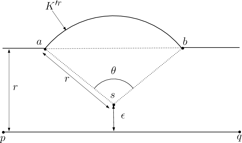
The proof of this theorem is given in Sections 6, 7 and 8. We show in Figure 2 that this bound is tight. Furthermore, in the 33-dimensional case, this result also holds for the anisotropic curvature measure H~¯\overline{\widetilde{H}}.

Now, if we take the function f⁡(x)=max⁡(1−‖x−c‖/r,0)f(x)=\max(1-\|x-c\|/r,0) equal to 11 at a point c∈∂Kr′c\in\partial K^{\prime}_{r} that radially decreases in a “small” ball 𝔹{\mathbb{B}} of radius rr and vanishes out of 𝔹{\mathbb{B}}, then we can get local information about the curvature of Kr′K^{\prime}_{r} from the curvature of KrK_{r} in the neighborhood of cc.

We also note that the conclusion of the theorem may be rephrased by saying that the bounded Lipschitz distance between the curvature measures of KrK_{r} and Kr′K^{\prime}_{r} is bounded by O⁡(ϵ)O(\sqrt{\epsilon}). The bounded Lipschitz distance between measures is similar to the Wasserstein distance (also called earth’s mover distance), except that it applies to general signed measures whereas Wasserstein distance is limited to probability measures. We refer to [8] for precise definitions.
Refer to caption

Figure 2: Tightness of the bound: we take K=[p,q]K=[p,q] and K′=[p,q]∪{s}K^{\prime}=[p,q]\cup\{s\}, where ss is at a distance ϵ\epsilon from KK. We have dH​(K,K′)=ϵd_{H}(K,K^{\prime})=\epsilon and the total curvature θ\theta of Kr′K^{\prime}_{r} between aa and bb satisfies θ=2​arccos⁡(r−ϵr)=O⁡(ϵ).\theta=2\arccos\left(\frac{r-\epsilon}{r}\right)=O\left(\sqrt{\epsilon}\right).

4.2 General result

The result of the previous section ensuring the stability of the curvature measures assume that both the compact sets KK and K′K^{\prime} have sufficiently large μ\mu-reach. Nevertheless, in practical settings, particularly when dealing with point clouds, such an hypothesis is rarely satisfied. Using Theorem 1, it is still possible to approximate the curvature measures of the offsets of a compact set with positive μ\mu-reach from any sufficiently close approximation of it.

Theorem 5

Let KK and K′K^{\prime} be two compact subsets of ℝd\mathbb{R}^{d} such that rμ​(K′)>rr_{\mu}(K^{\prime})>r. Assume that the Hausdorff distance ε=dH​(K,K′){\varepsilon}=d_{H}(K,K^{\prime}) between KK and K′K^{\prime} is such that ε<μ260+9​μ2​r{\varepsilon}<\frac{\mu^{2}}{60+9\mu^{2}}r. Then the conclusions of Theorem 4 also hold.

Of course, if for s>0s>0, the compact set K′K^{\prime} satisfies rμ​(Ks′)>c>0r_{\mu}(K^{\prime}_{s})>c>0, the same theorem applies to Ks′K^{\prime}_{s}. Furthermore, thanks to Theorem 1, the value of rμ​(Ks′)r_{\mu}(K^{\prime}_{s}) can be read on the critical function of the sample KK.

Proof :
It follows from Theorem 1 (the critical values separation theorem of [6]) that the critical function of KK is greater than μ2\frac{\mu}{2} on the interval (16​εμ2,r−3​ε​r)\left(\frac{16{\varepsilon}}{\mu^{2}},r-3\sqrt{{\varepsilon}r}\right). Note that since μ>μ2\mu>\frac{\mu}{2}, the critical function of KK is also greater than μ2\frac{\mu}{2} on the same interval. As a consequence the two compact sets K~=K16​εμ2\tilde{K}=K_{\frac{16{\varepsilon}}{\mu^{2}}} and K~′=K16​εμ2′\tilde{K}^{\prime}=K^{\prime}_{\frac{16{\varepsilon}}{\mu^{2}}} have their μ2\frac{\mu}{2}-reach greater than r−3​ε​r−16​εμ2r-3\sqrt{{\varepsilon}r}-\frac{16{\varepsilon}}{\mu^{2}}. Notice that for any δ>0\delta>0, K~δ=K16​εμ2+δ\tilde{K}_{\delta}=K_{\frac{16{\varepsilon}}{\mu^{2}}+\delta} and since dH​(K,K′)=εd_{H}(K,K^{\prime})={\varepsilon} then dH​(K~,K~′)≤εd_{H}(\tilde{K},\tilde{K}^{\prime})\leq{\varepsilon}. To apply Theorem 4 to K~\tilde{K} and K~′\tilde{K}^{\prime}, μ2\frac{\mu}{2} and rr, the Hausdorff distance ε{\varepsilon} between K~\tilde{K} and K~′\tilde{K}^{\prime} must satisfy 0<ε<2−28​μ2​(r−3​ε​r−16​εμ2)0<{\varepsilon}<\frac{2-\sqrt{2}}{8}\mu^{2}(r-3\sqrt{{\varepsilon}r}-\frac{16{\varepsilon}}{\mu^{2}}) (note that since μ2≤12\frac{\mu}{2}\leq\frac{1}{2}, min⁡(μ,12)=μ\min(\mu,\frac{1}{2})=\mu). One easily checks (by computing the solutions of the inequality and using that for all 0≤x≤10\leq x\leq 1, 1−x≥1−x2\sqrt{1-x}\geq 1-\frac{x}{2}) that this inequality is implied by the assumption made on ε{\varepsilon}. The theorem now follows immediately from Theorem 4. □\Box

Remark that in the previous proof, the choice of μ2\frac{\mu}{2} to apply the critical values separation theorem of [6] and then the theorem 4 is arbitrary. The same proof can be given replacing μ2\frac{\mu}{2} by any 0<μ′<μ0<\mu^{\prime}<\mu leading to somewhat different, but more technical, constraints on ε{\varepsilon} and rr in the statement of Theorem 4.

5 Computation of the curvature measures of 3​D3D point clouds

5.1 Gaussian and mean curvature measures of 3​D3D point clouds

Let KK be a finite set of points in ℝ3\mathbb{R}^{3} and r>0r>0. We assume that the set of balls of radius rr and centered in KK are in general position (as in [17]): no 44 points lie on a common plane; no 55 points lie on a common sphere; and the smallest sphere through any 2, 3 or 4 points of KK has a radius different from rr. In the 33-dimensional case, we denote by Φ𝒞H=Φ𝒞1\Phi^{H}_{\mathcal{C}}=\Phi^{1}_{\mathcal{C}} the mean curvature measure and by Φ𝒞G=Φ𝒞2\Phi^{G}_{\mathcal{C}}=\Phi^{2}_{\mathcal{C}} the gaussian curvature measure.

Note that the boundary of the union of balls KrK_{r} is a spherical polyhedron: its faces are spherical polygons contained in the spheres of radius rr centered on points of KK; its edges are arcs of circles contained in the intersection of pairs of spheres of radius rr centered on KK; its vertices belong to the intersection of three spheres of radius rr and centered in KK. It follows from Lemma 2.2 in [18] that the combinatorial structure of ∂Kr\partial K_{r} is in one-to-one correspondence with the boundary of the α\alpha-shape of KK for α=r\alpha=r. As a consequence, under the general position assumption, to compute ΦKrG​(f)\Phi^{G}_{K_{r}}(f) and ΦKrH​(f)\Phi^{H}_{K_{r}}(f), it is sufficient to compute the curvature measures Φ𝒞G​(f)\Phi^{G}_{\mathcal{C}}(f) and Φ𝒞H​(f)\Phi^{H}_{\mathcal{C}}(f), where 𝒞\mathcal{C} is the union of one, two or three balls of radius rr. The orientation of the boundary of the union of ball is taken so that the normal is pointing outside. All the curvature measures for the union of one, two or three balls are given respectively in Propositions 1, 2 and 3.

Proposition 1

Let 𝔹{\mathbb{B}} be a ball of radius rr of ℝ3\mathbb{R}^{3} and let BB be a Borel set of ℝ3\mathbb{R}^{3}. Then the curvature measures of 𝔹{\mathbb{B}} above BB are given by:

Φ𝔹H​(B)=2r​A​r​e​a​(B∩∂𝔹)a​n​dΦ𝔹G​(B)=1r2​A​r​e​a​(B∩∂𝔹).\Phi^{H}_{{\mathbb{B}}}(B)=\frac{2}{r}\ Area(B\cap\partial{\mathbb{B}})\quad and\quad\Phi^{G}_{{\mathbb{B}}}(B)=\frac{1}{r^{2}}\ Area(B\cap\partial{\mathbb{B}}).

Proof :
Since ∂𝔹\partial{\mathbb{B}} is a smooth surface, one has

Φ𝔹H​(B)=∫B∩∂𝔹H⁡(p)​𝑑p=2r​A​r​e​a​(B∩∂𝔹)\Phi^{H}_{{\mathbb{B}}}(B)=\int_{B\cap\partial{\mathbb{B}}}H(p)dp=\frac{2}{r}\ Area(B\cap\partial{\mathbb{B}})

and

Φ𝔹G​(B)=∫B∩∂𝔹G⁡(p)​𝑑p=1r2​A​r​e​a​(B∩∂𝔹),\Phi^{G}_{{\mathbb{B}}}(B)=\int_{B\cap\partial{\mathbb{B}}}G(p)dp=\frac{1}{r^{2}}\ Area(B\cap\partial{\mathbb{B}}),

where G⁡(p)G(p) is the Gaussian curvature and H⁡(p)H(p) is the mean curvature of 𝔹{\mathbb{B}} at pp. □\Box
In the following, we use the notation: ωH=ω1\omega^{H}=\omega_{1} and ωG=ω2\omega^{G}=\omega_{2}.

Proposition 2

Let 𝔹1{\mathbb{B}}_{1} and 𝔹2{\mathbb{B}}_{2} be two intersecting balls of ℝ3\mathbb{R}^{3}, of same radius r>0r>0 and of centers A1A_{1} and A2A_{2}, and CC be the circle ∂𝔹1∩∂𝔹2\partial{\mathbb{B}}_{1}\cap\partial{\mathbb{B}}_{2}. Let BB be a ball of ℝ3\mathbb{R}^{3}. Then the curvature measures of 𝔹1∪𝔹2{\mathbb{B}}_{1}\cup{\mathbb{B}}_{2} above B∩CB\cap C are given by:

Φ𝔹1∪𝔹2H​(B∩C)=−2​β​r​a​r​c​s​i​n​(A1​A22​r)​1−(A1​A22​r)2\Phi^{H}_{{\mathbb{B}}_{1}\cup{\mathbb{B}}_{2}}(B\cap C)=-2\beta r\ arcsin\left(\frac{A_{1}A_{2}}{2r}\right)\sqrt{1-\left(\frac{A_{1}A_{2}}{2r}\right)^{2}}

and

Φ𝔹1∪𝔹2G​(B∩C)=−β​A1​A2r,\Phi^{G}_{{\mathbb{B}}_{1}\cup{\mathbb{B}}_{2}}(B\cap C)=-\frac{\beta\ A_{1}A_{2}}{r},

where β=2​π​l​e​n​g​t​h​(B∩C)l​e​n​g​t​h​(C)\beta=2\pi\frac{length(B\cap C)}{length(C)} is the angle of the arc of circle B∩CB\cap C.

Proof :
Since the normal cycle is additive and since CC is one-dimensional, one has:

Φ𝔹1∪𝔹2H​(B∩C)=Φ𝔹1H​(B∩C)+Φ𝔹2H​(B∩C)−Φ𝔹1∩𝔹2H​(B∩C)=−Φ𝔹1∩𝔹2H​(B∩C).\begin{array}[]{rl}\Phi^{H}_{{\mathbb{B}}_{1}\cup{\mathbb{B}}_{2}}(B\cap C)&=\Phi^{H}_{{\mathbb{B}}_{1}}(B\cap C)+\Phi^{H}_{{\mathbb{B}}_{2}}(B\cap C)-\Phi^{H}_{{\mathbb{B}}_{1}\cap{\mathbb{B}}_{2}}(B\cap C)\\ &=-\Phi^{H}_{{\mathbb{B}}_{1}\cap{\mathbb{B}}_{2}}(B\cap C).\end{array}

We now need to describe the normal cycle of 𝔹1∩𝔹2{\mathbb{B}}_{1}\cap{\mathbb{B}}_{2} “above” C∩BC\cap B. Since 𝔹1∩𝔹2{\mathbb{B}}_{1}\cap{\mathbb{B}}_{2} is convex, its normal cycle “above” C∩BC\cap B is just the 22-current defined by integration over the set:

SC(𝔹1∩𝔹2)={(m,ξ),m∈C∩B,∥ξ∥=1and∀q∈𝔹1∩𝔹2m​q→.ξ≤0}.S_{C}({\mathbb{B}}_{1}\cap{\mathbb{B}}_{2})=\left\{(m,\xi),\ m\in C\cap B,\ \|\xi\|=1\ and\ \forall q\in{\mathbb{B}}_{1}\cap{\mathbb{B}}_{2}\ \overrightarrow{mq}.\xi\leq 0\right\}.

Let α=a​r​c​s​i​n​(A1​A22​r)\alpha=arcsin\left(\frac{A_{1}A_{2}}{2r}\right). In an suitable frame, the set SC​(𝔹1∩𝔹2)S_{C}({\mathbb{B}}_{1}\cap{\mathbb{B}}_{2}) can be parametrized by:

f:[0,β]×[−α,α]→ℝ3×𝕊2(u,v)↦((r​cos⁡α​cos⁡ur​cos⁡α​sin⁡u0),sin⁡(v)​(001)+cos⁡(v)​(cos⁡usin⁡u0))\begin{array}[]{rlll}f:&[0,\beta]\times[-\alpha,\alpha]&\to&\mathbb{R}^{3}\times\mathbb{S}^{2}\\ &(u,v)&\mapsto&\left(\begin{array}[]{cc}\left(\begin{array}[]{c}r\cos\alpha\cos u\\ r\cos\alpha\sin u\\ 0\end{array}\right),\sin(v)\ \left(\begin{array}[]{c}0\\ 0\\ 1\end{array}\right)+\cos(v)\ \left(\begin{array}[]{c}\cos u\\ \sin u\\ 0\end{array}\right)\end{array}\right)\end{array}

Let (m,ξ)=f⁡(u,v)∈S⁡(𝔹1∩𝔹2)(m,\xi)=f(u,v)\in S({\mathbb{B}}_{1}\cap{\mathbb{B}}_{2}). We put

e1=(−sin⁡ucos⁡u0)​ and ​e2=cos⁡(v)​(001)−sin⁡(v)​(cos⁡usin⁡u0).e_{1}=\left(\begin{array}[]{c}-\sin u\\ \cos u\\ 0\end{array}\right)\mbox{ and }e_{2}=\cos(v)\ \left(\begin{array}[]{c}0\\ 0\\ 1\end{array}\right)-\sin(v)\ \left(\begin{array}[]{c}\cos u\\ \sin u\\ 0\end{array}\right).

Then (e1,e2,ξ)(e_{1},e_{2},\xi) is a direct orthonormal basis of ℝ3\mathbb{R}^{3}. We put ϵ1=(e1,0)\epsilon_{1}=(e_{1},0), ϵ2=(e2,0)\epsilon_{2}=(e_{2},0), ϵ1~=(0,e1)\widetilde{\epsilon_{1}}=(0,e_{1}) and ϵ2~=(0,e2)\widetilde{\epsilon_{2}}=(0,e_{2}). On has [14]:

ωH=ϵ1∧ϵ2~+ϵ1~∧ϵ2andωG=ϵ1~∧ϵ2~.\omega^{H}=\epsilon_{1}\wedge\widetilde{\epsilon_{2}}+\widetilde{\epsilon_{1}}\wedge\epsilon_{2}\quad\mbox{and}\quad\omega^{G}=\widetilde{\epsilon_{1}}\wedge\widetilde{\epsilon_{2}}.

Furthermore, one has:

∂f∂u​(u,v)=(r​cos⁡α​e1,cos⁡v​e1)and∂f∂v​(u,v)=(0,e2).\frac{\partial f}{\partial u}(u,v)=(r\cos\alpha\ e_{1},\cos v\ e_{1})\quad\mbox{and}\quad\frac{\partial f}{\partial v}(u,v)=(0,e_{2}).

We then have:

f∗​ωH​((1,0),(0,1))=ωH​(∂f∂u​(u,v),∂f∂v​(u,v))=r​cos⁡α,f^{*}\omega^{H}((1,0),(0,1))=\omega^{H}\left(\frac{\partial f}{\partial u}(u,v),\frac{\partial f}{\partial v}(u,v)\right)=r\cos\alpha,
f∗​ωG​((1,0),(0,1))=cos⁡v.f^{*}\omega^{G}((1,0),(0,1))=\cos v.

Then

Φ𝔹1∪𝔹2H(C)=−∫0β∫−ααrcosαdudv=−2βrαcosα.\Phi^{H}_{{\mathbb{B}}_{1}\cup{\mathbb{B}}_{2}}(C)=-\int_{0}^{\beta}\int_{-\alpha}^{\alpha}r\cos\alpha\ dudv=-2\beta r\alpha\cos\alpha.

Similarly, one has:

Φ𝔹1∪𝔹2G(C)=−∫0β∫−ααcosvdudv=−2βsinα=−β​A1​A2r.\Phi^{G}_{{\mathbb{B}}_{1}\cup{\mathbb{B}}_{2}}(C)=-\int_{0}^{\beta}\int_{-\alpha}^{\alpha}\cos v\ dudv=-2\beta\sin\alpha=-\frac{\beta\ A_{1}A_{2}}{r}.

□\Box

Proposition 3

Let 𝔹1{\mathbb{B}}_{1}, 𝔹2{\mathbb{B}}_{2} and 𝔹3{\mathbb{B}}_{3} be three intersecting balls of ℝ3\mathbb{R}^{3}, of radius rr, of centers A1A_{1}, A2A_{2} and A3A_{3}, and p∈∂𝔹1∩∂𝔹2∩∂𝔹3p\in\partial{\mathbb{B}}_{1}\cap\partial{\mathbb{B}}_{2}\cap\partial{\mathbb{B}}_{3}. Then the curvature measures of 𝔹1∪𝔹2∪𝔹3{\mathbb{B}}_{1}\cup{\mathbb{B}}_{2}\cup{\mathbb{B}}_{3} above pp are given by:

Φ𝔹1∪𝔹2∪𝔹3H​({p})=0\Phi^{H}_{{\mathbb{B}}_{1}\cup{\mathbb{B}}_{2}\cup{\mathbb{B}}_{3}}(\{p\})=0\

and

Φ𝔹1∪𝔹2∪𝔹3G​({p})=4​arctan⁡tan⁡(σ2)​tan⁡(σ−α1,22)​tan⁡(σ−α2,32)​tan⁡(σ−α1,32),\Phi^{G}_{{\mathbb{B}}_{1}\cup{\mathbb{B}}_{2}\cup{\mathbb{B}}_{3}}(\{p\})=4\ \arctan\sqrt{\tan\left(\frac{\sigma}{2}\right)\tan\left(\frac{\sigma-\alpha_{1,2}}{2}\right)\tan\left(\frac{\sigma-\alpha_{2,3}}{2}\right)\tan\left(\frac{\sigma-\alpha_{1,3}}{2}\right)},

where

σ=α1,2+α2,3+α3,12αi,j=∠⁡(p​Ai→,p​Aj→)=2​a​r​c​s​i​n​(Ai​Aj2​r),\begin{array}[]{l}\sigma=\frac{\alpha_{1,2}+\alpha_{2,3}+\alpha_{3,1}}{2}\\ \alpha_{i,j}=\angle\left(\overrightarrow{pA_{i}},\overrightarrow{pA_{j}}\right)=2\ arcsin\left(\frac{A_{i}A_{j}}{2r}\right),\end{array}

Proof :
Since the 2-form ωH\omega^{H} is mixed and since the support of the normal cycle of 𝔹1∪𝔹2∪𝔹3{\mathbb{B}}_{1}\cup{\mathbb{B}}_{2}\cup{\mathbb{B}}_{3} “above” pp lies in {p}×ℝ3\{p\}\times\mathbb{R}^{3}, one has Φ𝔹1∪𝔹2H​({p})=0\Phi^{H}_{{\mathbb{B}}_{1}\cup{\mathbb{B}}_{2}}(\{p\})=0. Since the normal cycle is additive and since {p}\{p\} is 0-dimensional, by using Proposition 2, one has:

Φ𝔹1∪𝔹2∪𝔹3G​({p})=Φ𝔹1G​({p})+Φ𝔹2G​({p})+Φ𝔹3G​({p})−Φ𝔹1∩𝔹2G​({p})−Φ𝔹1∩𝔹3G​({p})−Φ𝔹2∩𝔹3G​({p})+Φ𝔹1∩𝔹2∩𝔹3G​({p}).=Φ𝔹1∩𝔹2∩𝔹3G​({p}).\begin{array}[]{rrl}\Phi^{G}_{{\mathbb{B}}_{1}\cup{\mathbb{B}}_{2}\cup{\mathbb{B}}_{3}}(\{p\})&=&\Phi^{G}_{{\mathbb{B}}_{1}}(\{p\})+\Phi^{G}_{{\mathbb{B}}_{2}}(\{p\})+\Phi^{G}_{{\mathbb{B}}_{3}}(\{p\})\\ &&-\Phi^{G}_{{\mathbb{B}}_{1}\cap{\mathbb{B}}_{2}}(\{p\})-\Phi^{G}_{{\mathbb{B}}_{1}\cap{\mathbb{B}}_{3}}(\{p\})-\Phi^{G}_{{\mathbb{B}}_{2}\cap{\mathbb{B}}_{3}}(\{p\})\\ &&+\Phi^{G}_{{\mathbb{B}}_{1}\cap{\mathbb{B}}_{2}\cap{\mathbb{B}}_{3}}(\{p\}).\\ &=&\Phi^{G}_{{\mathbb{B}}_{1}\cap{\mathbb{B}}_{2}\cap{\mathbb{B}}_{3}}(\{p\}).\end{array}

Φ𝔹1∩𝔹2∩𝔹3G​({p})\Phi^{G}_{{\mathbb{B}}_{1}\cap{\mathbb{B}}_{2}\cap{\mathbb{B}}_{3}}(\{p\}) is just the area of the set:

S(p)={(p,ξ),∥ξ∥=1and∀q∈𝔹1∩𝔹2∩𝔹3p​q→.ξ≤0}.S(p)=\left\{(p,\xi),\ \|\xi\|=1\ and\ \forall q\in{\mathbb{B}}_{1}\cap{\mathbb{B}}_{2}\cap{\mathbb{B}}_{3}\ \overrightarrow{pq}.\xi\leq 0\right\}.

The set S⁡(p)S(p) is a spherical triangle whose area is given by the following formulae (see [1] page 289):

4​arctan⁡tan⁡(σ2)​tan⁡(σ−α1,22)​tan⁡(σ−α2,32)​tan⁡(σ−α1,32).4\ \arctan\sqrt{\tan\left(\frac{\sigma}{2}\right)\tan\left(\frac{\sigma-\alpha_{1,2}}{2}\right)\tan\left(\frac{\sigma-\alpha_{2,3}}{2}\right)\tan\left(\frac{\sigma-\alpha_{1,3}}{2}\right)}.

□\Box

In Figure 3, we sampled a non-manifold compact set. It is interesting to note that both the mean and the gaussian curvature are low (and negative) in the middle of the disc. This is due to the fact that the curvature is “caught” by a function ff whose support traverses the disc and intersects the cube.

Refer to caption     Refer to caption

Refer to caption     Refer to caption

Figure 3: The mean (left) and gaussian (right) curvatures of a point cloud PP sampling a non smooth compact set union of a solid cube with a disc and an arc circle. The colors vary from green (minimum value of the curvature) to red (maximum value of the curvature) passing through blue. The curvature measures are computed using our approach for a fixed offset value of α=0.1\alpha=0.1 (the diameter of the point cloud being equal to 22). A curvature value is assigned to each data point pp by integration of a Lipschitz function with support contained in a ball of center pp and radius 0.30.3. These values are then used to color the faces of the boundary of the α\alpha-shape of PP (top) or the offset of the point cloud (bottom).

Figure 4 also illustrates the algorithm for a sampling of the union of a torus and a cube.

Refer to caption     Refer to caption

Figure 4: The mean (left) and gaussian (right) curvatures of a point cloud PP sampling the union of a solid cube and a solid torus. The colors vary from green (minimum value of the curvature) to red (maximum value of the curvature) passing through blue. The curvature measures are computed using our approach for a fixed offset value of α=0.1\alpha=0.1 (the diameter of the point cloud being equal to 22). A curvature value is assigned to each data point pp by integration of a Lipschitz function with support contained in a ball of center pp and radius 0.30.3. These values are then used to color the faces of the boundary of the α\alpha-shape of PP.

The algorithm
In practice, we use a halfedge data structure (provided by S. Loriot from INRIA Sophia-Antipolis) for the representation of the boundary of the union of balls KrK_{r}. Let now ff be a Lipschitz function on ℝd\mathbb{R}^{d}. To compute the isotropic curvature measures ΦKrG​(f)\Phi^{G}_{K_{r}}(f) and ΦKrH​(f)\Phi^{H}_{K_{r}}(f) of the union of balls KrK_{r}, we triangulate ∂Kr\partial K_{r}. More precisely, we triangulate every face of ∂Kr\partial K_{r} into “small” spherical patches of diameter less than η\eta. We then approximate ff by a function f~\tilde{f} that is constant on each “small” patch and that coincides with ff in at least one point of each patch. We then calculate the isotropic curvature measures with f~\tilde{f} “above the faces” by using Proposition 1. Similarly, by using Proposition 2, we calculate the isotropic curvature measures above the “spherical edges” with a function f~\tilde{f} piecewise constant on “small” edges of lengths less than η\eta. Finally, we calculate exactly the isotropic curvature measures “above” the vertices by using Proposition 3.

Numerical integration
Let B′B^{\prime} be a borel subset of ℝ3\mathbb{R}^{3} that contains the support of the functions ff and let B=B′∩∂KrB=B^{\prime}\cap\partial K_{r}. The numerical error done by approximating ff by a piecewise constant function f~\tilde{f} is then given by:

|ΦKrG​(f)−ΦKrG​(f~)|≤L​i​p​(f)​M​(N⁡(Kr)​⌞​(B×ℝd))​η|\Phi^{G}_{K_{r}}(f)-\Phi^{G}_{K_{r}}(\tilde{f})|\leq Lip(f)\ M(N(K_{r})\llcorner(B\times\mathbb{R}^{d}))\ \eta

and

|ΦKrH​(f)−ΦKrH​(f~)|≤L​i​p​(f)​M​(N⁡(Kr)​⌞​(B×ℝd))​η|\Phi^{H}_{K_{r}}(f)-\Phi^{H}_{K_{r}}(\tilde{f})|\leq Lip(f)\ M(N(K_{r})\llcorner(B\times\mathbb{R}^{d}))\ \eta

where f~\tilde{f} is constant on each patch and coincides with ff at at least one point in the patch.

Proof: We show the result for the Gaussian curvature measure. The proof for the mean curvature measure is similar. One has:

|ΦKrG​(f)−ΦKrG​(f~)|=∫s​p​t​(N⁡(Kr))∩(B×ℝd)(f¯−f~¯)​ωG≤sup(p,n)∈(B×ℝd)‖f¯​(p,n)−f~¯​(p,n)‖​M​(N⁡(Kr)​⌞​(B×ℝd)).\begin{array}[]{rl}|\Phi^{G}_{K_{r}}(f)-\Phi^{G}_{K_{r}}(\tilde{f})|&\displaystyle=\int_{spt(N(K_{r}))\cap(B\times\mathbb{R}^{d})}(\bar{f}-\bar{\tilde{f}})\ \omega^{G}\\ &\displaystyle\leq\sup_{(p,n)\in(B\times\mathbb{R}^{d})}\|\bar{f}(p,n)-\bar{\tilde{f}}(p,n)\|\ M(N(K_{r})\llcorner(B\times\mathbb{R}^{d})).\end{array}

Let FF be a face of the spherical polygon ∂Kr∩B′\partial K_{r}\cap B^{\prime}, that is decomposed into spherical patches Δ\Delta. Let f~\tilde{f} be the piecewise constant function equal to f⁡(p0)f(p_{0}) on every spherical patch Δ\Delta of FF (with p0∈Δp_{0}\in\Delta). We then have:

sup(p,n)∈(F×ℝd)‖f¯​(p,n)−f~¯​(p,n)‖≤L​i​p​(f)​supΔ⊂FηΔ,\sup_{(p,n)\in(F\times\mathbb{R}^{d})}\|\bar{f}(p,n)-\bar{\tilde{f}}(p,n)\|\leq Lip(f)\ \sup_{\Delta\subset F}\eta_{\Delta},

where ηΔ\eta_{\Delta} is the length of the longest edge of Δ\Delta. The result is similar for a spherical edge CC of ∂Kr∩B′\partial K_{r}\cap B^{\prime}: if one decomposes CC into small arc of circles ee one has:

sup(p,n)∈(C×ℝd)‖f¯​(p,n)−f~¯​(p,n)‖≤L​i​p​(f)​supe⊂Cl⁡(e),\sup_{(p,n)\in(C\times\mathbb{R}^{d})}\|\bar{f}(p,n)-\bar{\tilde{f}}(p,n)\|\leq Lip(f)\ \sup_{e\subset C}l(e),

where l⁡(e)l(e) is the length of the arc of circle ee.

5.2 Anisotropic curvature measures of 3​D3D point clouds

In the previous section, we described an algorithm that allows to calculate the curvature measures ΦKrG​(f)\Phi^{G}_{K_{r}}(f) and ΦKrH​(f)\Phi^{H}_{K_{r}}(f) when KK is a finite set of points. Similarly, one can also calculate the anisotropic curvature measure H¯Kr​(f)\overline{H}_{K_{r}}(f) and H~¯Kr​(f)\overline{\widetilde{H}}_{K_{r}}(f) of KrK_{r} by using the curvature measures formulae for the union of one, two or three balls (see Propositions 4, 5 and 6). More details on how to use these formulae can be found in [14, 15].

Proposition 4

Let 𝔹{\mathbb{B}} be a ball of ℝ3\mathbb{R}^{3} and let BB be a Borel set of ℝ3\mathbb{R}^{3}. Then the anisotropic curvature measures of 𝔹{\mathbb{B}} above BB are given by the 3×33\times 3-matrix:

H~¯𝔹​(B)=H¯𝔹​(B)=∫B∩∂𝔹1r​(I​d−np​npt)​𝑑p,\overline{\widetilde{H}}_{{\mathbb{B}}}(B)=\overline{H}_{{\mathbb{B}}}(B)=\int_{B\cap\partial{\mathbb{B}}}\frac{1}{r}\ (Id-n_{p}{}^{t}n_{p})\ dp,

where I​dId is the identity matrix of ℝ3\mathbb{R}^{3}, npn_{p} is the unitary normal of 𝔹{\mathbb{B}} at pp and npt{}^{t}n_{p} its transpose.

Proof :
Let X,YX,Y be two vectors of ℝ3\mathbb{R}^{3} and PpP_{p} denotes the projection onto the plane tangent to 𝔹{\mathbb{B}} at the point pp. Using that Pp​(X)=X−<X,np>​npP_{p}(X)=X-<X,n_{p}>n_{p}, we have:

H¯𝔹​(B)​(X,Y)=∫B∩∂𝔹Hp​(Pp​(X),Pp​(Y))​𝑑p=∫B∩∂𝔹1r​(I​d−np​npt)​𝑑p.\overline{H}_{{\mathbb{B}}}(B)(X,Y)=\int_{B\cap\partial{\mathbb{B}}}H_{p}(P_{p}(X),P_{p}(Y))dp=\int_{B\cap\partial{\mathbb{B}}}\frac{1}{r}\ (Id-n_{p}{}^{t}n_{p})\ dp.

□\Box

Proposition 5

Let 𝔹1{\mathbb{B}}_{1} and 𝔹2{\mathbb{B}}_{2} be two intersecting balls of ℝ3\mathbb{R}^{3}, of same radius r>0r>0 and of centers A1A_{1} and A2A_{2}, and CC be the circle ∂𝔹1∩∂𝔹2\partial{\mathbb{B}}_{1}\cap\partial{\mathbb{B}}_{2}. Let BB be a ball of ℝ3\mathbb{R}^{3}. Then the anisotropic curvature measures of 𝔹1∪𝔹2{\mathbb{B}}_{1}\cup{\mathbb{B}}_{2} above B∩CB\cap C are given by the 3×33\times 3 matrix H¯𝔹1∪𝔹2​(B∩C)\overline{H}_{{\mathbb{B}}_{1}\cup{\mathbb{B}}_{2}}(B\cap C):

−r​sin⁡α​(12​(α−sin⁡2​α2)​(β+sin⁡2​β2)(α−sin⁡2​α2)​1−cos⁡2​β40(α−sin⁡2​α2)​1−cos⁡2​β412​(α−sin⁡2​α2)​(β−sin⁡2​β2)000β⁡(α+sin⁡2​α2)),-r\sin\alpha\left(\begin{array}[]{ccc}\frac{1}{2}\left(\alpha-\frac{\sin 2\alpha}{2}\right)\left(\beta+\frac{\sin 2\beta}{2}\right)&\left(\alpha-\frac{\sin 2\alpha}{2}\right)\frac{1-\cos 2\beta}{4}&0\\ \left(\alpha-\frac{\sin 2\alpha}{2}\right)\frac{1-\cos 2\beta}{4}&\frac{1}{2}\left(\alpha-\frac{\sin 2\alpha}{2}\right)\left(\beta-\frac{\sin 2\beta}{2}\right)&0\\ 0&0&\beta\left(\alpha+\frac{\sin 2\alpha}{2}\right)\end{array}\right),

and the 3×33\times 3 matrix H~¯𝔹1∪𝔹2​(B∩C)\overline{\widetilde{H}}_{{\mathbb{B}}_{1}\cup{\mathbb{B}}_{2}}(B\cap C):

r​α​sin⁡α​((β−sin⁡2​β2)cos⁡2​β−120cos⁡2​β−12(β−sin⁡2​β2)0000),r\alpha\sin\alpha\left(\begin{array}[]{ccc}\left(\beta-\frac{\sin 2\beta}{2}\right)&\frac{\cos 2\beta-1}{2}&0\\ \frac{\cos 2\beta-1}{2}&\left(\beta-\frac{\sin 2\beta}{2}\right)&0\\ 0&0&0\end{array}\right),

in the orthonormal frame (0,i,j,k)(0,i,j,k) where (0,i,j)(0,i,j) generates the plane of the circle CC and ii points toward one on the two extremities of the arc of circle B∩CB\cap C, where α\alpha and β\beta are defined as in the proof of Proposition 2.

Proof :
We take the same notations that the ones of Proposition 2. We have:

H¯𝔹1∪𝔹2​(B∩C)​(X,Y)=∫0β∫−ααf∗​ωX,Y.\overline{H}_{{\mathbb{B}}_{1}\cup{\mathbb{B}}_{2}}(B\cap C)(X,Y)=\int_{0}^{\beta}\int_{-\alpha}^{\alpha}f^{*}\omega^{X,Y}.

As in Proposition 2, we take (m,ξ)=f⁡(u,v)∈SC​(𝔹1∩𝔹2)(m,\xi)=f(u,v)\in S_{C}({\mathbb{B}}_{1}\cap{\mathbb{B}}_{2}). We have:

f∗​ωX,Y​((1,0),(0,1))=ω(m,ξ)X,Y​(∂f∂u​(u,v),∂f∂v​(u,v))=(0,Y)∧(ξ×X,0)​((r​sin⁡α​e1,cos⁡v​e1),(0,e2))=|(0,Y).(r​sin⁡α​e1,cos⁡v​e1)(ξ×X,0).(r​sin⁡α​e1,cos⁡v​e1)(0,Y).(0,e2)(ξ×X,0).(0,e2)|=|cos⁡v​Y.e1det(ξ,X,r​sin⁡α​e1)Y.e20|=−r​sin⁡α​X.e2​Y.e2.\begin{array}[]{rl}f^{*}\omega^{X,Y}((1,0),(0,1))&=\omega^{X,Y}_{(m,\xi)}\left(\frac{\partial f}{\partial u}(u,v),\frac{\partial f}{\partial v}(u,v)\right)\\ &=(0,Y)\ \wedge(\xi\times X,0)((r\sin\alpha\ e_{1},\cos v\ e_{1}),(0,e_{2}))\\ &=\left|\begin{array}[]{cc}(0,Y).(r\sin\alpha\ e_{1},\cos v\ e_{1})&(\xi\times X,0).(r\sin\alpha\ e_{1},\cos v\ e_{1})\\ (0,Y).(0,e_{2})&(\xi\times X,0).(0,e_{2})\\ \end{array}\right|\\ &=\left|\begin{array}[]{cc}\cos v\ Y.e_{1}&\det(\xi,X,r\sin\alpha e_{1})\\ Y.e_{2}&0\\ \end{array}\right|\\ &=-r\sin\alpha\ X.e_{2}\ Y.e_{2}.\\ \end{array}

The result is thus obtained by integrating the matrix of e2​e2te_{2}{}^{t}e_{2} given by:

(sin2⁡v​cos2⁡usin2⁡v​sin⁡u​cos⁡u−sin⁡v​cos⁡v​cos⁡usin2⁡v​sin⁡u​cos⁡usin2⁡v​sin2⁡u−sin⁡v​sin⁡u​cos⁡v−cos⁡v​sin⁡v​cos⁡u−cos⁡v​sin⁡v​sin⁡ucos2⁡v).\left(\begin{array}[]{ccc}\sin^{2}v\cos^{2}u&\sin^{2}v\sin u\cos u&-\sin v\cos v\cos u\\ \sin^{2}v\sin u\cos u&\sin^{2}v\sin^{2}u&-\sin v\sin u\cos v\\ -\cos v\sin v\cos u&-\cos v\sin v\sin u&\cos^{2}v\\ \end{array}\right).

Similarly, we have:

f∗​ω~X,Y​((1,0),(0,1))=r​sin⁡α​X.e1​Y.e1.f^{*}\widetilde{\omega}^{X,Y}((1,0),(0,1))=r\sin\alpha\ X.e_{1}\ Y.e_{1}.

The result for H~¯𝔹1∪𝔹2​(B∩C)\overline{\widetilde{H}}_{{\mathbb{B}}_{1}\cup{\mathbb{B}}_{2}}(B\cap C) is thus obtained by integrating the matrix of e1​e1te_{1}{}^{t}e_{1} given by:

(sin2⁡u−sin⁡u​cos⁡u0−sin⁡u​cos⁡ucos2⁡u0000).\left(\begin{array}[]{ccc}\sin^{2}u&-\sin u\cos u&0\\ -\sin u\cos u&\cos^{2}u&0\\ 0&0&0\\ \end{array}\right).

□\Box

Proposition 6

Let 𝔹1{\mathbb{B}}_{1}, 𝔹2{\mathbb{B}}_{2} and 𝔹3{\mathbb{B}}_{3} be three intersecting balls of ℝ3\mathbb{R}^{3}, of radius rr, of centers A1A_{1}, A2A_{2} and A3A_{3}, and p∈∂𝔹1∩∂𝔹2∩∂𝔹3p\in\partial{\mathbb{B}}_{1}\cap\partial{\mathbb{B}}_{2}\cap\partial{\mathbb{B}}_{3}. Then the anisotropic curvature measures of 𝔹1∪𝔹2∪𝔹3{\mathbb{B}}_{1}\cup{\mathbb{B}}_{2}\cup{\mathbb{B}}_{3} above pp are equal to 00:

H¯𝔹1∪𝔹2∪𝔹3​({p})=0​a​n​d​H~¯𝔹1∪𝔹2∪𝔹3​({p})=0\overline{H}_{{\mathbb{B}}_{1}\cup{\mathbb{B}}_{2}\cup{\mathbb{B}}_{3}}(\{p\})=0\ and\ \overline{\widetilde{H}}_{{\mathbb{B}}_{1}\cup{\mathbb{B}}_{2}\cup{\mathbb{B}}_{3}}(\{p\})=0\

Proof :
The two forms ωX,Y\omega^{X,Y} and ω~X,Y\widetilde{\omega}^{X,Y} being mixed, they vanish on the normal component. □\Box

6 About the normal cycle of a compact of ℝd\mathbb{R}^{d}

In this section, we give preliminary results for compact sets in ℝd\mathbb{R}^{d}: in Lemma 2, we bound the mass of the normal cycle of a set whose boundary is of class 𝒞1\mathcal{C}^{1}; in Lemma 3, we recall a result of Zähle et al. that allows to define, under several assumptions, the normal cycle of a set whose complement has positive reach; in Lemma 4, we give relationships between the normal cycle of a set whose complement has positive reach and the normal cycle of its offset.

We first give the following lemma (that is a direct consequence of the Isotopy Lemma, Proposition 1.8 in [26]):

Lemma 1

Let KK be a compact of ℝd\mathbb{R}^{d}. If rr is not a critical point of the distance function (i.e. χK​(r)≠0\chi_{K}(r)\neq 0), we then have:

{x,dK​(x)<r}¯={x,dK​(x)≤r}and{x,dK​(x)>r}¯={x,dK​(x)≥r}.\overline{\{x,\ d_{K}(x)<r\}}=\{x,\ d_{K}(x)\leq r\}\quad\mbox{and}\quad\overline{\{x,\ d_{K}(x)>r\}}=\{x,\ d_{K}(x)\geq r\}.
Lemma 2

Let XX be a compact subset of ℝd\mathbb{R}^{d} whose boundary is a hypersurface with positive reach RR. We then have:

M⁡(N⁡(X))≤(1+1R2)d−12​ℋd−1​(∂X).M(N(X))\leq\left(1+\frac{1}{R^{2}}\right)^{\frac{d-1}{2}}\ \mathcal{H}^{d-1}(\partial X).

More precisely, if B′B^{\prime} is a Borel of ℝd\mathbb{R}^{d} and B=B′∩∂XB=B^{\prime}\cap\partial X, we have:

M⁡[N⁡(X)​⌞​(B×ℝd)]≤(1+1R2)d−12​ℋd−1​(B).M\left[N(X)\llcorner(B\times\mathbb{R}^{d})\right]\leq\left(1+\frac{1}{R^{2}}\right)^{\frac{d-1}{2}}\ \mathcal{H}^{d-1}(B).

Proof :
Let us consider the following map:

f:B→s​p​t​(N⁡(X))∩(B×ℝd)m↦(m,n⁡(m)).\begin{array}[]{rclc}f:&B&\to&spt(N(X))\cap(B\times\mathbb{R}^{d})\\ &m&\mapsto&\left(m,n(m)\right)\end{array}.

Since the reach, and therefore the curvature of the surface ∂X\partial X is bounded by RR, it follows that the map m↦n⁡(m)m\mapsto n(m) is 1R\frac{1}{R}-Lipschitz. That implies that ff is also 1+1R2\sqrt{1+\frac{1}{R^{2}}}-Lipschitz. Since the map ff is one-to-one, the general coarea formulae (see Theorem 4.2 of [30] or Proposition 3.13 of [29]) states that:

M⁡(N⁡(X)​⌞​(B×ℝd))=∫s​p​t​(N⁡(X))∩(B×ℝd)d​ℋd−1=∫BJd−1​(f)​d​ℋd−1≤∫B(1+1R2)d−12​d​ℋd−1≤(1+1R2)d−12​ℋd−1​(B).\begin{array}[]{rl}\displaystyle M(N(X)\llcorner(B\times\mathbb{R}^{d}))&\displaystyle=\int_{spt(N(X))\cap(B\times\mathbb{R}^{d})}d\mathcal{H}^{d-1}\\ &\displaystyle=\int_{B}J_{d-1}(f)\ d\mathcal{H}^{d-1}\\ &\displaystyle\leq\int_{B}\ \left(1+\frac{1}{R^{2}}\right)^{\frac{d-1}{2}}\ d\mathcal{H}^{d-1}\\ &\displaystyle\leq\left(1+\frac{1}{R^{2}}\right)^{\frac{d-1}{2}}\ \mathcal{H}^{d-1}(B).\end{array}

where Jd−1​(f)J_{d-1}(f) is the (d-1)-jacobian of the Lipschitz map ff (see [29], page 24-25). □\Box

Under certain assumptions, Rataj and Zähle [34] showed that the closure of the complement of a compact set with positive reach admits a normal cycle. More precisely, we denote by ii the inversion map

i:ℝd×𝕊d−1→ℝd×𝕊d−1(x,n)↦(x,−n),\begin{array}[]{rclc}i:&\mathbb{R}^{d}\times\mathbb{S}^{d-1}&\to&\mathbb{R}^{d}\times\mathbb{S}^{d-1}\\ &(x,n)&\mapsto&(x,-n),\\ \end{array}

and by i♯i_{\sharp} the push-forward by ii. We define the erosions X−ϵX_{-\epsilon} of XX by X−ϵ=(Xc¯ϵ)c¯X_{-\epsilon}=\overline{\left(\overline{X^{c}}_{\,\epsilon}\right)^{c}}. We then get the following lemma by combining results of Zähle et al. [33, 34] and [7]:

Lemma 3

Let KK be a compact set of ℝd\mathbb{R}^{d} with μ\mu-reach greater than rr and let X=KrX=K_{r}. We can then define the normal cycle of XX as the flat limit of its erosions as follows:

ℱ(N(X−ϵ)−N(X))⟶ϵ→00.\mathcal{F}\left(N\left(X_{-\epsilon}\right)-N(X)\right)\longrightarrow_{\epsilon\to 0}0.

Furthermore, since Xc¯\overline{X^{c}} has positive reach, it has a normal cycle and we have:

N⁡(X)=−i♯​N​(Xc¯)andM⁡(N⁡(X))=M⁡(N⁡(Xc¯)).N(X)=-i_{\sharp}N\left(\overline{X^{c}}\right)\quad\mbox{and}\quad M(N(X))=M\left(N\left(\overline{X^{c}}\right)\right).

Proof :
Proposition 2 and Theorem 3 of [34] imply that the normal cycle N⁡(X)N(X) of XX is well defined and we have:

ℱ(N(X−ϵ)−N(X))⟶ϵ→00.\mathcal{F}\left(N\left(X_{-\epsilon}\right)-N(X)\right)\longrightarrow_{\epsilon\to 0}0.

Now, since Xc¯\overline{X^{c}} has positive reach [7], Corollary 3.1 of [33] (or Proposition 4 of [34]) implies that:

ℱ[N(Xc¯)−(−i♯N(X−ϵ))]⟶ϵ→00.\mathcal{F}\left[N\left(\overline{X^{c}}\right)-\left(-i_{\sharp}N\left(X_{-\epsilon}\right)\right)\right]\longrightarrow_{\epsilon\to 0}0.

We then have

N⁡(X)=−i♯​N​(Xc¯).N(X)=-i_{\sharp}N\left(\overline{X^{c}}\right).

□\Box

We now consider the following map

Ft:ℝd×ℝd→ℝd×ℝd(x,v)↦(x+t​v,v),\begin{array}[]{cccc}F_{t}:&\mathbb{R}^{d}\times\mathbb{R}^{d}&\to&\mathbb{R}^{d}\times\mathbb{R}^{d}\\ &(x,v)&\mapsto&(x+tv,v)\\ \end{array},

and denote by Ft​♯F_{t\sharp} the associated push-forward for currents.

Lemma 4

Let VV be a compact set of ℝd\mathbb{R}^{d} with positive reach R>0R>0. We then have for ϵ<R\epsilon<R:

N⁡(V)=F−ϵ​♯​[N⁡(Vϵ)].N\left(V\right)=F_{-\epsilon\sharp}\left[N\left(V_{\,\epsilon}\right)\right].

That result can be localized. Let B′B^{\prime} be a Borel of ℝd\mathbb{R}^{d} and B=(B′×ℝd)∩s​p​t​(N⁡(V))B=(B^{\prime}\times\mathbb{R}^{d})\cap spt(N(V)). We then have:

N⁡(V)​⌞​B=F−ϵ​♯​[N⁡(Vϵ)​⌞​F−ϵ−1​(B)],N\left(V\right)\llcorner B=F_{-\epsilon\sharp}\left[N\left(V_{\,\epsilon}\right)\llcorner F_{-\epsilon}^{-1}(B)\right],

In particular, if KK is a compact set of ℝd\mathbb{R}^{d} with μ\mu-reach greater than rr, X=KrX=K_{r}, the set V=Xc¯V=\overline{X^{c}} has a reach R>μ​rR>\mu r, and we have for ϵ<R\epsilon<R:

N⁡(X)=−i♯​N​(Xc¯)=−i♯​F−ϵ​♯​[N⁡(Xc¯ϵ)]andM⁡(N⁡(X))≤(1+ϵ2)d−12​M​[N⁡(Xc¯ϵ)].\begin{array}[]{rl}&N\left(X\right)=-i_{\sharp}N\left(\overline{X^{c}}\right)=-i_{\sharp}F_{-\epsilon\sharp}\left[N\left(\overline{X^{c}}_{\,\epsilon}\right)\right]\\ \mbox{and}&M\left(N\left(X\right)\right)\leq\left(1+\epsilon^{2}\right)^{\frac{d-1}{2}}\ M\left[N\left(\overline{X^{c}}_{\,\epsilon}\right)\right].\\ \end{array}

Let now B′B^{\prime} be a Borel of ℝd\mathbb{R}^{d} and B=(B′×ℝd)∩s​p​t​(N⁡(X))B=(B^{\prime}\times\mathbb{R}^{d})\cap spt(N(X)). We then have:

N⁡(X)​⌞​B=−i♯​F−ϵ​♯​[N⁡(Xc¯ϵ)​⌞​F−ϵ−1​(i⁡(B))],N\left(X\right)\llcorner B=-i_{\sharp}F_{-\epsilon\sharp}\left[N\left(\overline{X^{c}}_{\,\epsilon}\right)\llcorner F_{-\epsilon}^{-1}(i(B))\right],
M⁡(N⁡(X)​⌞​B)≤(1+ϵ2)d−12​M​[N⁡(Xc¯ϵ)​⌞​F−ϵ−1​(i⁡(B))].M\left(N\left(X\right)\llcorner B\right)\leq\left(1+\epsilon^{2}\right)^{\frac{d-1}{2}}\ M\left[N\left(\overline{X^{c}}_{\,\epsilon}\right)\llcorner F_{-\epsilon}^{-1}(i(B))\right].

Proof :
We notice that the restriction of F−ϵF_{-\epsilon} to the support of N⁡(Vϵ)N\left(V_{\,\epsilon}\right) is a one-to-one map:

F−ϵ:s​p​t​(N⁡(Vϵ))→s​p​t​(N⁡(V))(x,v)↦(x−ϵ​v,v).\begin{array}[]{cccc}F_{-\epsilon}:&spt\left(N\left(V_{\,\epsilon}\right)\right)&\to&spt\left(N\left(V\right)\right)\\ &(x,v)&\mapsto&(x-\epsilon v,v)\\ \end{array}.

The general coarea formula implies that:

M⁡(N⁡(V))=∫s​p​t​(N⁡(V))d​ℋd−1=∫s​p​t​(N⁡(Vϵ))Jd−1​(F−ϵ)​d​ℋd−1.M\left(N\left(V\right)\right)=\int_{spt\left(N\left(V\right)\right)}d\mathcal{H}^{d-1}=\int_{spt\left(N\left(V_{\,\epsilon}\right)\right)}J_{d-1}(F_{-\epsilon})\ d\mathcal{H}^{d-1}.

The map F−ϵF_{-\epsilon} is 1+ϵ2\sqrt{1+\epsilon^{2}}-Lipschitz, thus we have Jd−1​(F−ϵ)≤(1+ϵ2)d−12J_{d-1}(F_{-\epsilon})\leq\left(1+\epsilon^{2}\right)^{\frac{d-1}{2}} and:

M⁡(N⁡(V))≤(1+ϵ2)d−12​M​(N⁡(Vϵ)).M\left(N\left(V\right)\right)\leq\left(1+\epsilon^{2}\right)^{\frac{d-1}{2}}\ M\left(N\left(V_{\epsilon}\right)\right).

More precisely, for any d−1d-1-differential form φ\varphi on ℝd×ℝd\mathbb{R}^{d}\times\mathbb{R}^{d}, one has:

F−ϵ​♯​N​(Vϵ)​(φ)=N⁡(Vϵ)​(F−ϵ∗​φ)=∫s​p​t​(N⁡(Vϵ))(F−ϵ∗​φ)x​(e1x∧…∧ed−1x)​d​ℋd−1​(x)=∫s​p​t​(N⁡(Vϵ))φF−ϵ​(x)​((D​F−ϵ​(x)​e1x)∧…∧(D​F−ϵ​(x)​ed−1x))​d​ℋd−1​(x)=∫s​p​t​(N⁡(Vϵ))Jd−1​(F−ϵ)​(x)​φF−ϵ​(x)​((D​F−ϵ​(x)​e1x)∧…∧(D​F−ϵ​(x)​ed−1x)|(D​F−ϵ​(x)​e1x)∧…∧(D​F−ϵ​(x)​ed−1x)|)​d​ℋd−1​(x)=∫s​p​t​(N⁡(Vϵ))Jd−1​(F−ϵ)​(x)​φF−ϵ​(x)​(e1F−ϵ​(x)∧…∧ed−1F−ϵ​(x))​d​ℋd−1​(x)=∫s​p​t​(N⁡(V))φy(e1y∧…∧ed−1y)dℋd−1(y) (by the general coarea formula)=N​(V)​(φ),\begin{array}[]{rl}F_{-\epsilon\sharp}N\left(V_{\,\epsilon}\ \right)(\varphi)&=N\left(V_{\,\epsilon}\ \right)\left(F_{-\epsilon}^{*}\varphi\right)\\ &\displaystyle=\int_{spt\left(N\left(V_{\,\epsilon}\right)\right)}(F_{-\epsilon}^{*}\varphi)_{x}(e_{1}^{x}\wedge...\wedge e_{d-1}^{x})\ d\mathcal{H}^{d-1}(x)\\ &\displaystyle=\int_{spt\left(N\left(V_{\,\epsilon}\right)\right)}\varphi_{F_{-\epsilon}(x)}((DF_{-\epsilon}(x)e_{1}^{x})\wedge...\wedge(DF_{-\epsilon}(x)e_{d-1}^{x}))\ d\mathcal{H}^{d-1}(x)\\ &\displaystyle=\int_{spt\left(N\left(V_{\,\epsilon}\right)\right)}J_{d-1}(F_{-\epsilon})(x)\ \varphi_{F_{-\epsilon}(x)}\left(\frac{(DF_{-\epsilon}(x)e_{1}^{x})\wedge...\wedge(DF_{-\epsilon}(x)e_{d-1}^{x})}{|(DF_{-\epsilon}(x)e_{1}^{x})\wedge...\wedge(DF_{-\epsilon}(x)e_{d-1}^{x})|}\right)\ d\mathcal{H}^{d-1}(x)\\ &\displaystyle=\int_{spt\left(N\left(V_{\,\epsilon}\right)\right)}J_{d-1}(F_{-\epsilon})(x)\ \varphi_{F_{-\epsilon}(x)}\left(e_{1}^{F_{-\epsilon}(x)}\wedge...\wedge e_{d-1}^{F_{-\epsilon}(x)}\right)\ d\mathcal{H}^{d-1}(x)\\ &\displaystyle=\int_{spt\left(N\left(V\right)\right)}\varphi_{y}\left(e_{1}^{y}\wedge...\wedge e_{d-1}^{y}\right)\ d\mathcal{H}^{d-1}(y)\quad\mbox{\ (by the general coarea formula)}\\ &\displaystyle=N\left(V\right)\left(\varphi\right),\\ \end{array}

where e1x∧..∧ed−1xe_{1}^{x}\wedge..\wedge e_{d-1}^{x} is a unit (d-1)-vector associated with the oriented tangent space Tx​(s​p​t​(N⁡(Vϵ)))T_{x}\left(spt\left(N\left(V_{\,\epsilon}\right)\right)\right) and e1y∧..∧ed−1ye_{1}^{y}\wedge..\wedge e_{d-1}^{y} is a unit (d-1)-vector associated with the oriented tangent space Ty​(s​p​t​(N​(V)))T_{y}\left(spt\left(N\left(V\right)\right)\right) and Jd−1​(F−ϵ)​(x)=|(D​F−ϵ​(x)​e1x)∧…∧(D​F−ϵ​(x)​ed−1x)|J_{d-1}(F_{-\epsilon})(x)=|(DF_{-\epsilon}(x)e_{1}^{x})\wedge...\wedge(DF_{-\epsilon}(x)e_{d-1}^{x})| ℋd−1\mathcal{H}^{d-1}-almost everywhere. That implies that:

N⁡(V)=F−ϵ​♯​N​(Vϵ).N\left(V\right)=F_{-\epsilon\sharp}N\left(V_{\,\epsilon}\right).

The local version is done the same way by noticing that the restriction of F−ϵF_{-\epsilon} to the support of N⁡(Vϵ)​⌞​F−ϵ−1​(B)N\left(V_{\,\epsilon}\right)\llcorner F_{-\epsilon}^{-1}(B) is a one-to-one map:

F−ϵ:s​p​t​(N⁡(Vϵ)​⌞​F−ϵ−1​(B))→s​p​t​(N⁡(V)​⌞​B)(x,v)↦(x−ϵ​v,v).\begin{array}[]{cccc}F_{-\epsilon}:&spt\left(N\left(V_{\,\epsilon}\right)\llcorner F_{-\epsilon}^{-1}(B)\right)&\to&spt\left(N\left(V\right)\llcorner B\right)\\ &(x,v)&\mapsto&(x-\epsilon v,v)\\ \end{array}.

□\Box

7 Normal cycles of the double offsets of two close compact sets

The aim of this section is to prove the following proposition. It states that if two compact sets KK and K′K^{\prime} are close in the Hausdorff sense, then the normal cycles of their double offsets are close for the flat norm. This result is local since we evaluate the normal cycles locally.

More precisely, let B′B^{\prime} be a Borel subset of ℝd\mathbb{R}^{d} and B=B′∩∂Kr,t′B=B^{\prime}\cap\partial K^{\prime}_{r,t}. We consider in the following the normal cycles of Kr,tK_{r,t} and Kr,t′K^{\prime}_{r,t} restricted to BB and π⁡(B)\pi(B), where π\pi is the projection onto Kr,tK_{r,t}. We consider the two currents D′=N⁡(Kr,t′)​⌞​(B×ℝd)D^{\prime}=N(K^{\prime}_{r,t})\llcorner(B\times\mathbb{R}^{d}) and D=N⁡(Kr,t)​⌞​(π⁡(B)×ℝd)D=N(K_{r,t})\llcorner(\pi(B)\times\mathbb{R}^{d}) given by:

D′​(φ)=∫s​p​t​(N⁡(Kr,t′))∩(B×ℝd)φandD⁡(φ)=∫s​p​t​(N⁡(Kr,t))∩(π⁡(B)×ℝd)φ,\begin{array}[]{rl}&\displaystyle D^{\prime}(\varphi)=\int_{spt(N(K^{\prime}_{r,t}))\cap(B\times\mathbb{R}^{d})}\varphi\\ \mbox{and}&\displaystyle D(\varphi)=\int_{spt(N(K_{r,t}))\cap(\pi(B)\times\mathbb{R}^{d})}\varphi,\end{array}

for any (d-1)-differential form φ\varphi of ℝd×ℝd\mathbb{R}^{d}\times\mathbb{R}^{d}.

Proposition 7

Let KK and K′K^{\prime} be two compact sets of ℝd\mathbb{R}^{d} whose μ\mu-reaches are greater than rr. We suppose that the Hausdorff distance ϵ=dH​(K,K′)\epsilon=d_{H}(K,K^{\prime}) between KK and K′K^{\prime} is less than r​μ​(2−2)2​min⁡(μ,12)\frac{r\mu\ (2-\sqrt{2})}{2}\min(\mu,\frac{1}{2}). For t∈[ϵmin⁡(μ,12)​(2−2),r​μ2]t\in\left[\frac{\epsilon}{\min(\mu,\frac{1}{2})\ (2-\sqrt{2})},\frac{r\mu}{2}\right], we can write:

D′−D=∂R1+R2D^{\prime}-D=\partial R_{1}+R_{2}

where R1R_{1} and R2R_{2} are currents satisfying

M⁡(R1)\displaystyle M(R_{1}) ≤\displaystyle\leq M⁡(D′)​k1​k2\displaystyle M(D^{\prime})k_{1}k_{2}
M⁡(R2)\displaystyle M(R_{2}) ≤\displaystyle\leq M⁡(∂D′)​k1​k2,\displaystyle M(\partial D^{\prime})k_{1}k_{2},

where

k1\displaystyle k_{1} =\displaystyle= 1+(1+t2(t−ϵμ)2)d−12\displaystyle 1+\left(\frac{1+t^{2}}{\left(t-\frac{\epsilon}{\mu}\right)^{2}}\right)^{\frac{d-1}{2}}
k2\displaystyle k_{2} =\displaystyle= (ϵμ)2+900​ϵμ​t.\displaystyle\sqrt{\left(\frac{\epsilon}{\mu}\right)^{2}+900\frac{\epsilon}{\mu t}}.

In particular the flat norm of D−D′D-D^{\prime} is bounded by (M⁡(D′)+M⁡(∂D′))​k1​k2(M(D^{\prime})+M(\partial D^{\prime}))k_{1}k_{2}.

The proof of that proposition relies on the two following lemmas:

Lemma 5

Let XX and X′X^{\prime} be two compact sets of ℝd\mathbb{R}^{d} with reaches greater than R>0R>0. Let t≤R2t\leq\frac{R}{2} and ϵ=dH​(X,X′)\epsilon=d_{H}(X,X^{\prime}). If ϵ≤t2\epsilon\leq\frac{t}{2}, then for any xx at a distance tt from XX, we have:

2​sin⁡∠⁡(∇X(x),∇X′(x))2≤30​ϵt.2\sin\frac{\angle\left(\nabla_{X}(x),\nabla_{X^{\prime}}(x)\right)}{2}\leq 30\sqrt{\frac{\epsilon}{t}}.

Proof :
For ρ\rho such that 0<ρ<t0<\rho<t, we denote by GX​(x,ρ)G_{X}(x,\rho), as in section 5 of [5], the convex hull for every y∈B⁡(x,ρ)y\in B(x,\rho) of all the “classical” gradients ∇X(y)\nabla_{X}(y) of the distance function dXd_{X}. By using Theorem 5.6 in [5], we have that:

∇X′(x)∈GX​(x,ρ)ρ2​d​(x,X′)+2​ϵρ.\nabla_{X^{\prime}}(x)\in G_{X}(x,\rho)_{\frac{\rho}{2d(x,X^{\prime})}+\frac{2\epsilon}{\rho}}. (3)

On another hand we know ([22] page 435) that the projection map πX\pi_{X} on XX is RR−(t+ρ)\frac{R}{R-(t+\rho)}-Lipschitz for points at distance less than (t+ρ)(t+\rho) from XX. Then, for y∈B⁡(x,ρ)y\in B(x,\rho) one has d⁡(x,y)≤ρd(x,y)\leq\rho and d⁡(πX​(x),πX​(y))≤R​ρR−(t+ρ)d(\pi_{X}(x),\pi_{X}(y))\leq\frac{R\rho}{R-(t+\rho)} and:

‖y​πX​(y)→−x​πX​(x)→‖≤ρ+R​ρR−(t+ρ).\|\overrightarrow{y\pi_{X}(y)}-\overrightarrow{x\pi_{X}(x)}\|\leq\rho+\frac{R\rho}{R-(t+\rho)}.

Using the fact that ∇X(z)=−1‖z​πX​(z)→‖​z​πX​(z)→\nabla_{X}(z)=\frac{-1}{\|\overrightarrow{z\pi_{X}(z)}\|}\overrightarrow{z\pi_{X}(z)} one get, for y∈B⁡(x,ρ)y\in B(x,\rho):

‖∇X(y)−∇X(x)‖≤1t−ρ​(ρ+R​ρR−(t+ρ)).\|\nabla_{X}(y)-\nabla_{X}(x)\|\leq\frac{1}{t-\rho}\left(\rho+\frac{R\rho}{R-(t+\rho)}\right).

This and Equation(3) gives:

2​sin⁡∠​∇X(x),∇X′(x)2=‖∇X(x)−∇X′(x)‖≤ρt−ρ​(1+RR−(t+ρ))+ρ2​(t−ϵ)+2​ϵρ.2\sin\frac{\angle\nabla_{X}(x),\nabla_{X^{\prime}}(x)}{2}=\|\nabla_{X}(x)-\nabla_{X^{\prime}}(x)\|\leq\frac{\rho}{t-\rho}\left(1+\frac{R}{R-(t+\rho)}\right)+\frac{\rho}{2(t-\epsilon)}+\frac{2\epsilon}{\rho}.

Taking ρ=ϵ​t\rho=\sqrt{\epsilon t} and ϵ≤t2\epsilon\leq\frac{t}{2} one gets:

2​sin⁡∠​∇X(x),∇X′(x)2≤(11−22​(1+11−12​(1+22))+3)​ϵt≤30​ϵt.2\sin\frac{\angle\nabla_{X}(x),\nabla_{X^{\prime}}(x)}{2}\leq\left(\frac{1}{1-\frac{\sqrt{2}}{2}}\left(1+\frac{1}{1-\frac{1}{2}\left(1+\frac{\sqrt{2}}{2}\right)}\right)+3\right)\sqrt{\frac{\epsilon}{t}}\leq 30\sqrt{\frac{\epsilon}{t}}.

□\Box

Lemma 6

Let KK and K′K^{\prime} be two compact sets of ℝd\mathbb{R}^{d} whose μ\mu-reaches are greater than rr. Then for every t∈(0,r​μ)t\in(0,r\mu), we have:

dH​(Kr,t,Kr,t′)≤ϵμanddH​(∂Kr,t,∂Kr,t′)≤ϵμ.d_{H}(K_{r,t},K^{\prime}_{r,t})\leq\frac{\epsilon}{\mu}\quad\mbox{and}\quad d_{H}(\partial K_{r,t},\partial K^{\prime}_{r,t})\leq\frac{\epsilon}{\mu}.

Proof :
First remark that if we take two compact sets AA and BB with μ~\tilde{\mu}-reach greater than rr, such that dH​(A,B)≤ϵ~d_{H}(A,B)\leq\tilde{\epsilon}, one has:

dH​((Ar)c¯,(Br)c¯)≤ϵ~μ~d_{H}\left(\overline{(A_{r})^{c}},\overline{(B_{r})^{c}}\right)\leq\frac{\tilde{\epsilon}}{\tilde{\mu}} (4)

Indeed, let x∈Ar¯cx\in\overline{A_{r}}^{c}. Then d⁡(x,A)≥rd(x,A)\geq r and d⁡(x,B)≥r−ϵ~d(x,B)\geq r-\tilde{\epsilon}. Let s↦σ⁡(s)s\mapsto\sigma(s), σ⁡(0)=x\sigma(0)=x be the trajectory of ∇B\nabla_{B} issued from xx and parametrized by arc-length. While σ⁡(s)∈Br\sigma(s)\in B_{r}, we have [28]:

dB​(σ⁡(s))=dB​(x)+∫0s‖∇B(σ⁡(s))‖​𝑑s≥r−ϵ~+s​μ~.d_{B}(\sigma(s))=d_{B}(x)+\int_{0}^{s}\|\nabla_{B}(\sigma(s))\|ds\geq r-\tilde{\epsilon}+s\tilde{\mu}.

We then have σ⁡(s)∈(Br)c¯\sigma(s)\in\overline{(B_{r})^{c}} for s≥ϵ~μ~s\geq\frac{\tilde{\epsilon}}{\tilde{\mu}}. As a consequence, there exists x′∈(Br)c¯x^{\prime}\in\overline{(B_{r})^{c}} such that d⁡(x,x′)≤ϵ~μ~d(x,x^{\prime})\leq\frac{\tilde{\epsilon}}{\tilde{\mu}}. We apply Equation (4) with A=KA=K and B=K′B=K^{\prime} and we get:

dH​((Kr)c¯,(Kr′)c¯)≤ϵμd_{H}\left(\overline{(K_{r})^{c}},\overline{(K^{\prime}_{r})^{c}}\right)\leq\frac{{\epsilon}}{\mu} (5)

We apply again Equation (4) with A=(Kr)c¯A=\overline{(K_{r})^{c}} and B=(Kr′)c¯B=\overline{(K^{\prime}_{r})^{c}} with ϵ~=ϵμ\tilde{\epsilon}=\frac{\epsilon}{\mu} and μ~=1\tilde{\mu}=1:

dH​(Kr,tc¯,Kr,t′c¯)≤ϵμ.d_{H}(\overline{{K_{r,t}}^{c}},\overline{{K^{\prime}_{r,t}}^{c}})\leq\frac{\epsilon}{\mu}.

Remark also that for any compact sets AA and BB, one has dH​(At,Bt)≤dH​(A,B)d_{H}(A_{t},B_{t})\leq d_{H}(A,B). Therefore, by Equation (5) one has:

dH​(Kr,t,Kr,t′)≤ϵμ.d_{H}({{K_{r,t}}},{{K^{\prime}_{r,t}}})\leq\frac{\epsilon}{\mu}.

The two last equations imply that

dH​(∂Kr,t,∂Kr,t′)≤ϵμ.d_{H}(\partial{{K_{r,t}}},\partial{{K^{\prime}_{r,t}}})\leq\frac{\epsilon}{\mu}.

Indeed, let x∈∂Kr,tx\in\partial K_{r,t}. Then xx is at a distance less than ϵμ\frac{\epsilon}{\mu} from Kr,t′K^{\prime}_{r,t} and Kr,t′c¯\overline{{K^{\prime}_{r,t}}^{c}}. Then, there exists y∈Kr,t′y\in K^{\prime}_{r,t} and z∈Kr,t′c¯z\in\overline{{K^{\prime}_{r,t}}^{c}} such that x​y≤ϵμxy\leq\frac{\epsilon}{\mu} and x​z≤ϵμxz\leq\frac{\epsilon}{\mu}. Since the line-segment [y​z][yz] intersects ∂Kr,t\partial K_{r,t}, there exists x′∈∂Kr,t′x^{\prime}\in\partial K^{\prime}_{r,t} such that x​x′≤ϵμxx^{\prime}\leq\frac{\epsilon}{\mu}. □\Box

Proof of Proposition 7
Let KK and K′K^{\prime} be two compact sets whose μ\mu-reaches are greater than rr. We put ϵ=dH​(K,K′)\epsilon=d_{H}(K,K^{\prime}). We suppose that ϵμ⁡(2−2)≤t≤r​μ2\frac{\epsilon}{\mu\ (2-\sqrt{2})}\leq t\leq\frac{r\mu}{2}. Lemma 6 then implies that

dH​(∂Kr,t,∂Kr,t′)≤ϵμ≤(2−2)​t.d_{H}(\partial K_{r,t},\partial K^{\prime}_{r,t})\leq\frac{\epsilon}{\mu}\leq(2-\sqrt{2})\ t.

Let UtU_{t} be the tubular neighborhood of ∂Kr,t\partial K_{r,t} of radius t≤r​e​a​c​h​(∂Kr,t)t\leq reach(\partial K_{r,t}). The projection map π\pi onto ∂Kr,t\partial K_{r,t} is then defined on UtU_{t}. We clearly have ∂Kr,t′⊂Ut\partial K^{\prime}_{r,t}\subset U_{t}. More precisely, the map π\pi induces a one-to-one map between ∂Kr,t′\partial K^{\prime}_{r,t} and ∂Kr,t\partial K_{r,t} (see Theorem 4.1 of [11]). We now define

ψ:Ut×ℝd→s​p​t​(N⁡(Kr,t))(x,n)↦(π⁡(x),nπ⁡(x)).\begin{array}[]{cccc}\psi:&U_{t}\times\mathbb{R}^{d}&\to&spt\left(N\left(K_{r,t}\right)\right)\\ &(x,n)&\mapsto&(\pi(x),n_{\pi(x)})\end{array}.

Let hh be the affine homotopy between ψ\psi and the identity (see Federer [21] 4.1.9 page 364)

h:[0,1]×(Ut×ℝd)→ℝd×ℝd(t,x)↦(1−t)​x+t​ψ​(x).\begin{array}[]{cccc}h:&[0,1]\times(U_{t}\times\mathbb{R}^{d})&\to&\mathbb{R}^{d}\times\mathbb{R}^{d}\\ &(t,x)&\mapsto&(1-t)x+t\psi(x)\\ \end{array}.

Since the map π:∂Kr,t′→∂Kr,t\pi:\partial K^{\prime}_{r,t}\to\partial K_{r,t} is one-to-one, the map ψ\psi also induces a one-to-one map between s​p​t​(D′)spt(D^{\prime}) and s​p​t​(D)spt(D). Therefore, similarly as in the proof of Lemma 4, one has:

ψ♯​D′=D.\psi_{\sharp}D^{\prime}=D.

According to Federer ([22], 4.1.9 page 363-364), we have:

D−D′=ψ♯​D′−i​d♯​D′=∂R1+R2D-D^{\prime}\ =\ \psi_{\sharp}D^{\prime}-id_{\sharp}D^{\prime}\ =\partial R_{1}+R_{2}

where R1=[h♯​([0,1]×D′)]R_{1}=\left[h_{\sharp}\left([0,1]\times D^{\prime}\right)\right] and R2=h♯​([0,1]×∂D′)R_{2}=h_{\sharp}([0,1]\times\partial D^{\prime}). Again by Federer ([22], 4.1.9 page 364) or Fanghua ([20] page 187), we get:

M⁡(h♯​([0,1]×D′))≤M⁡(D′)​sups​p​t​(D′)|ψ−i​d|​sups​p​t​(D′)|1+Jd−1​(ψ)|,M\left(h_{\sharp}\left([0,1]\times D^{\prime}\right)\right)\leq M\left(D^{\prime}\right)\ \displaystyle\sup_{spt\left(D^{\prime}\right)}|\psi-id|\ \displaystyle\sup_{spt\left(D^{\prime}\right)}|1+J_{d-1}(\psi)|,

and

M⁡(h♯​([0,1]×∂D′))≤M⁡(∂D′)​sups​p​t​(D′)|ψ−i​d|​sups​p​t​(D′)|1+Jd−1​(ψ)|,M\left(h_{\sharp}([0,1]\times\partial D^{\prime})\right)\leq M\left(\partial D^{\prime}\right)\ \displaystyle\sup_{spt\left(D^{\prime}\right)}|\psi-id|\ \displaystyle\sup_{spt\left(D^{\prime}\right)}|1+J_{d-1}(\psi)|,

where Jd−1​(ψ)J_{d-1}(\psi) stands for the (d-1)-dimensional jacobian (as defined in [29], page 24-25). By Lemma 6, the space component of ψ−i​d\psi-id is less than ϵμ\frac{\epsilon}{\mu}. By Lemma 5, the normal component of ψ−i​d\psi-id is less than 30​ϵμ​t30\sqrt{\frac{\epsilon}{\mu t}}. Thus

sups​p​t​(N⁡(Kr,t′))|ψ−i​d|≤(ϵμ)2+900​ϵμ​t.\displaystyle\sup_{spt\left(N\left(K^{\prime}_{r,t}\right)\right)}|\psi-id|\leq\sqrt{\left(\frac{\epsilon}{\mu}\right)^{2}+900\frac{\epsilon}{\mu t}}.

We can note that the jacobian of the space component of ψ\psi (i.e. the projection) is bounded by (tt−ϵμ)d−1\left(\frac{t}{t-\frac{\epsilon}{\mu}}\right)^{d-1}. The jacobian of the map x∈Kr,t↦nxx\in K_{r,t}\mapsto n_{x} is upper bounded by (1t)d−1\left(\frac{1}{t}\right)^{d-1} (where t≤μ​r2t\leq\frac{\mu r}{2} is the reach of ∂Kr,t\partial K_{r,t}). The jacobian of the normal component of ψ\psi is upper bounded by the product (1t​tt−ϵμ)d−1\left(\frac{1}{t}\ \frac{t}{t-\frac{\epsilon}{\mu}}\right)^{d-1}. We then have

sups​p​t​(N⁡(Kr,t′))|1+Jd−1​(ψ)|≤1+(1+t2(t−ϵμ)2)d−12.\displaystyle\sup_{spt\left(N\left(K^{\prime}_{r,t}\right)\right)}|1+J_{d-1}(\psi)|\leq 1+\left(\frac{1+t^{2}}{\left(t-\frac{\epsilon}{\mu}\right)^{2}}\right)^{\frac{d-1}{2}}.

By using the definition of the flat norm we have:

ℱ⁡(D−D′)≤M⁡(h♯​([0,1]×D′))+M⁡(h♯​([0,1]×∂D′)).\mathcal{F}\left(D-D^{\prime}\right)\leq M\left(h_{\sharp}\left([0,1]\times D^{\prime}\right)\right)+M\left(h_{\sharp}([0,1]\times\partial D^{\prime})\right).

which is upper bounded by:

(M⁡(D′)+M⁡(∂D′))​(1+(1+t2(t−ϵμ)2)d−12)​(ϵμ)2+900​ϵμ​t.\left(M\left(D^{\prime}\right)+M\left(\partial D^{\prime}\right)\right)\left(1+\left(\frac{1+t^{2}}{\left(t-\frac{\epsilon}{\mu}\right)^{2}}\right)^{\frac{d-1}{2}}\right)\sqrt{\left(\frac{\epsilon}{\mu}\right)^{2}+900\frac{\epsilon}{\mu t}}.

8 From double offset to offset

The aim of that section is to prove Theorem 4. We assume that ff is C1C^{1}, the general case being obtained by a limit argument. Let C=(s​p​t​(f)α×ℝd)∩s​p​t​(N⁡(Kr′))C=(spt(f)_{\alpha}\times\mathbb{R}^{d})\cap spt(N(K^{\prime}_{r})), where α\alpha is a positive real number that will be specified later and let B=Ft∘i⁡(C)B=F_{t}\circ i(C). Thanks to Lemma 4, we have:

N⁡(Kr′)​⌞​(i∘F−t​(B))=−i♯​F−t​♯​[N⁡(Kr,t′)​⌞​B].\begin{array}[]{rl}N\left(K^{\prime}_{r}\right)\llcorner(i\circ F_{-t}(B))&=-i_{\sharp}F_{-t\sharp}\left[N\left(K^{\prime}_{r,t}\right)\llcorner B\right]\end{array}.

and

N⁡(Kr)​⌞​(i∘F−t​(ψ⁡(B)))=−i♯​F−t​♯​[N⁡(Kr,t)​⌞​ψ​(B)].,\begin{array}[]{rl}N\left(K_{r}\right)\llcorner(i\circ F_{-t}(\psi(B)))&=-i_{\sharp}F_{-t\sharp}\left[N\left(K_{r,t}\right)\llcorner\psi(B)\right].\end{array},

where ψ\psi is defined in the proof of Proposition 7. Remark that we have N⁡(Kr,t′)​⌞​B=N⁡(Kr,t′)​⌞​(B~×ℝd)N\left(K^{\prime}_{r,t}\right)\llcorner B=N\left(K^{\prime}_{r,t}\right)\llcorner(\tilde{B}\times\mathbb{R}^{d}), and N⁡(Kr,t)​⌞​ψ​(B)=N⁡(Kr,t)​⌞​(π⁡(B~)×ℝd)N\left(K_{r,t}\right)\llcorner\psi(B)=N\left(K_{r,t}\right)\llcorner(\pi(\tilde{B})\times\mathbb{R}^{d}) where B~\tilde{B} is the projection of BB onto the first factor of ℝ3×ℝ3\mathbb{R}^{3}\times\mathbb{R}^{3} and π\pi is the projection onto ∂Kr,t\partial K_{r,t}. Hence, Proposition 7 allows us to write:

N⁡(Kr′)​⌞​(i∘F−t​(B))−N⁡(Kr)​⌞​(i∘F−t​(ψ⁡(B)))=−i♯​F−t​♯​(∂R1+R2),N\left(K^{\prime}_{r}\right)\llcorner(i\circ F_{-t}(B))-N\left(K_{r}\right)\llcorner(i\circ F_{-t}(\psi(B)))=-i_{\sharp}F_{-t\sharp}(\partial R_{1}+R_{2}),

where R1R_{1} and R2R_{2} satisfy certain properties. In particular, from the proof we see that R2=h♯​[(N⁡(Kr,t′)​⌞​∂B)×[0,1]]R_{2}=h_{\sharp}[(N(K^{\prime}_{r,t})\llcorner\partial B)\times[0,1]], where hh is the result of the linear interpolation between the identity and ψ\psi. Since i∘F−ti\circ F_{-t} is linear, we have

(i∘F−t)∘h=h′∘(i∘F−t,I​d[0,1]),(i\circ F_{-t})\circ h=h^{\prime}\circ\left(i\circ F_{-t},Id_{[0,1]}\right),

where h′h^{\prime} is the result of the linear interpolation between the identity and ψ′=i∘F−t∘ψ∘Ft∘i\psi^{\prime}=i\circ F_{-t}\circ\psi\circ F_{t}\circ i. We then have that −i♯F−t​♯(R2)=h♯′[(−i♯F−t​♯N(Kr,t′)⌞∂B)×[0,1]]-i_{\sharp}F_{-t\sharp}(R_{2})=h^{\prime}_{\sharp}[(-i_{\sharp}F_{-t\sharp}N(K^{\prime}_{r,t})\llcorner\partial B)\times[0,1]]. Noting that −i♯​F−t​♯​(N⁡(Kr,t′)​⌞​∂B)=N⁡(Kr′)​⌞​∂C-i_{\sharp}F_{-t\sharp}(N(K^{\prime}_{r,t})\llcorner\partial B)=N(K^{\prime}_{r})\llcorner\partial C, and choosing α>‖ψ′−I​d‖∞\alpha>||\psi^{\prime}-Id||_{\infty}, we see that the support of i♯​F−t​♯​R2i_{\sharp}F_{-t\sharp}R_{2} is included in the α\alpha-offset of s​p​t​(N⁡(Kr′)​⌞​∂C)spt(N(K^{\prime}_{r})\llcorner\partial C). Due to the choice of α\alpha, this subset does not meet s​p​t​(f)×ℝdspt(f)\times\mathbb{R}^{d}. As a consequence, for any differential form ω\omega, letting:

Δ=|<N⁡(Kr′)​⌞​(i∘F−t​(B)),f¯​ω>−<N⁡(Kr)​⌞​(i∘F−t​(ψ⁡(B))),f¯​ω>|,\Delta=|<N\left(K^{\prime}_{r}\right)\llcorner(i\circ F_{-t}(B)),\bar{f}\omega>-<N\left(K_{r}\right)\llcorner(i\circ F_{-t}(\psi(B))),\bar{f}\omega>|,

we have:

Δ\displaystyle\Delta ≤\displaystyle\leq |<i♯​F−t​♯​∂R1,f¯​ω>|\displaystyle|<i_{\sharp}F_{-t\sharp}\partial R_{1},\bar{f}\omega>|
≤\displaystyle\leq |<i♯F−t​♯R1,df¯∧ω+f¯dω>|\displaystyle|<i_{\sharp}F_{-t\sharp}R_{1},d\bar{f}\wedge\omega+\bar{f}d\omega>|
≤\displaystyle\leq M⁡(i♯​F−t​♯​R1)​(L​i​p​(f¯)​‖ω‖+‖d​ω‖)\displaystyle M(i_{\sharp}F_{-t\sharp}R_{1})(Lip(\bar{f})||\omega||+||d\omega||)
≤\displaystyle\leq (1+t2)d/2​M​(R1)​(L​i​p​(f)​‖ω‖+‖d​ω‖)\displaystyle(1+t^{2})^{d/2}M(R_{1})(Lip(f)||\omega||+||d\omega||)
≤\displaystyle\leq M⁡(N⁡(Kr,t′)​⌞​B)​k1​k2​(1+t2)d/2​(L​i​p​(f)​‖ω‖+‖d​ω‖),\displaystyle M(N(K^{\prime}_{r,t})\llcorner B)k_{1}k_{2}(1+t^{2})^{d/2}(Lip(f)||\omega||+||d\omega||),

the last two inequalities following from Lemma 4, Proposition 7, and the fact that L​i​p​(f)=L​i​p​(f¯)Lip(f)=Lip(\bar{f}). Now remark that i∘F−t​(B)=Ci\circ F_{-t}(B)=C and i∘F−t​(ψ⁡(B))=ψ′​(C)i\circ F_{-t}(\psi(B))=\psi^{\prime}(C) respectively contain s​p​t​(N⁡(Kr′))∩(s​p​t​(f)×ℝd)spt(N(K^{\prime}_{r}))\cap(spt(f)\times\mathbb{R}^{d}) and s​p​t​(N⁡(Kr))∩(s​p​t​(f)×ℝd)spt(N(K_{r}))\cap(spt(f)\times\mathbb{R}^{d}), due to the choice of α\alpha. Hence we have:

Δ=|<N⁡(Kr′),f¯​ω>−<N⁡(Kr),f¯​ω>|.\Delta=|<N\left(K^{\prime}_{r}\right),\bar{f}\omega>-<N\left(K_{r}\right),\bar{f}\omega>|.

The quantity M⁡(N⁡(Kr,t′)​⌞​B)M(N(K^{\prime}_{r,t})\llcorner B) may be bounded above using Lemma 2:

M⁡(N⁡(Kr,t′)​⌞​B)\displaystyle M(N(K^{\prime}_{r,t})\llcorner B) ≤\displaystyle\leq (1+r​e​a​c​h​(∂Kr,t′)−2)d−12​ℋd−1​((∂Kr,t′)∩B′),\displaystyle(1+reach(\partial K^{\prime}_{r,t})^{-2})^{\frac{d-1}{2}}{\cal H}^{d-1}((\partial K^{\prime}_{r,t})\cap B^{\prime}),

where B′B^{\prime} is the preimage of s​p​t​(f)α∩Kr′spt(f)_{\alpha}\cap K^{\prime}_{r} under the projection on Kr′K^{\prime}_{r}. Since the reach of ∂Kr,t′\partial K^{\prime}_{r,t} may be bounded by a function of rr and μ\mu for t=r​μ/2t=r\mu/2, it only remains to bound the area term to finish the proof of Theorem 4. To do so, we use (a local version of) Theorem II.3 in [8], which yields the following bound in terms of covering numbers:

ℋd−1​((∂Kr,t′)∩B′)≤𝒩⁡(s​p​t​(f)α∩∂Kr′,t)​ωd−1​(2​t){\cal H}^{d-1}((\partial K^{\prime}_{r,t})\cap B^{\prime})\leq{\cal N}(spt(f)_{\alpha}\cap\partial K^{\prime}_{r},t)\ \omega_{d-1}(2t)

where ωd−1​(2​t)\omega_{d-1}(2t) denotes the surface area of the ball of radius 2​t2t in ℝd\mathbb{R}^{d}. Note now that 𝒩⁡(s​p​t​(f)α∩∂Kr′,t)≤𝒩⁡(s​p​t​(f)α,t){\cal N}(spt(f)_{\alpha}\cap\partial K^{\prime}_{r},t)\leq{\cal N}(spt(f)_{\alpha},t). The fact that α=O⁡(ϵ)\alpha=O(\sqrt{\epsilon}) easily follows from the following lemma:

Lemma 7
‖ψ′−I​d‖∞=O⁡(ϵ).\|\psi^{\prime}-Id\|_{\infty}=O(\sqrt{\epsilon}).

Proof :
Let (y′,n′)∈C(y^{\prime},n^{\prime})\in C and x′∈∂Kr,t′x^{\prime}\in\partial K^{\prime}_{r,t} be such that the projection of x′x^{\prime} onto K′rc¯\overline{{K^{\prime}}_{r}^{c}} is y′y^{\prime}. We put x=π⁡(x′)x=\pi(x^{\prime}) the projection of x′x^{\prime} onto ∂Kr,t\partial K_{r,t} and we denote by nn the normal to Kr,tK_{r,t} at the point xx that is pointing inside. We denote by yy the projection of xx onto Krc¯\overline{K_{r}^{c}}. We then have:

(x′,−n′)=Ft∘i(y′,n′),(x,−n)=ψ(x′,−n′)and(y,n)=i∘F−t(x,n)=ψ′(y′,n′).(x^{\prime},-n^{\prime})=F_{t}\circ i(y^{\prime},n^{\prime}),\quad(x,-n)=\psi(x^{\prime},-n^{\prime})\quad\mbox{and}\quad(y,n)=i\circ F_{-t}(x,n)=\psi^{\prime}(y^{\prime},n^{\prime}).

We now need to bound y​y′yy^{\prime} and ‖n−n′‖\|n-n^{\prime}\|. Lemma 5 implies that ‖n−n′‖=0​(ϵ)\|n-n^{\prime}\|=0(\sqrt{\epsilon}). We introduce y~\tilde{y} the projection of x′x^{\prime} onto Krc¯\overline{K_{r}^{c}}. Let us now bound y′​y~y^{\prime}\tilde{y} and y~​y\tilde{y}y.

Refer to caption

Figure 5: Proof of Lemma 7

Since x′∈∂Kr,t′x^{\prime}\in\partial K^{\prime}_{r,t}, we have x′​y′=tx^{\prime}y^{\prime}=t. Furthermore, by using Lemma 6, one has δ=x′​y~∈[t−ϵμ,t+ϵμ]\delta=x^{\prime}\tilde{y}\in\left[t-\frac{\epsilon}{\mu},t+\frac{\epsilon}{\mu}\right]. Let now denote by y′′y^{\prime\prime} the point of the half line issued from x′x^{\prime} and passing through y′y^{\prime}, that is at a distance δ\delta from x′x^{\prime}. We have by Lemma 5:

y′​y~≤y′​y′′+y′′​y~≤ϵμ+2​sin⁡∠⁡(∇Kr¯(x′),∇Kr′c¯(x′))2​(t+ϵμ)≤ϵμ+30​ϵμ​t​(t+ϵμ)=0​(ϵ).\begin{array}[]{rl}y^{\prime}\tilde{y}&\leq y^{\prime}y^{\prime\prime}+y^{\prime\prime}\tilde{y}\\ &\leq\frac{\epsilon}{\mu}+2\sin\frac{\angle\left(\nabla_{\overline{K_{r}}}(x^{\prime}),\nabla_{\overline{{K^{\prime}_{r}}^{c}}}(x^{\prime})\right)}{2}\ \left(t+\frac{\epsilon}{\mu}\right)\\ &\leq\frac{\epsilon}{\mu}+30\ \sqrt{\frac{\epsilon}{\mu t}}\ \left(t+\frac{\epsilon}{\mu}\right)\\ &=0\left(\sqrt{\epsilon}\right).\end{array}

Now by using again Lemma 6, one has x​x′≤ϵμxx^{\prime}\leq\frac{\epsilon}{\mu} and also that xx and x′x^{\prime} are at a distance less than (t+ϵμ)\left(t+\frac{\epsilon}{\mu}\right) from Krc¯\overline{K_{r}^{c}}. Since Krc¯\overline{K_{r}^{c}} has a reach greater than μ​r\mu r, then the projection map onto Krc¯\overline{K_{r}^{c}} is μ​rμ​r−(t+ϵμ)\frac{\mu r}{\mu r-\left(t+\frac{\epsilon}{\mu}\right)}-Lipschitz for points at a distance less than (t+ϵμ)\left(t+\frac{\epsilon}{\mu}\right) from Krc¯\overline{K_{r}^{c}} ([22] page 435). We then have:

y~​y≤ϵμ​μ​rμ​r−(t+ϵμ).\tilde{y}y\leq\frac{\epsilon}{\mu}\ \frac{\mu r}{\mu r-\left(t+\frac{\epsilon}{\mu}\right)}.

We then clearly have y​y′≤y′​y~+y~​y=0​(ϵ)yy^{\prime}\leq y^{\prime}\tilde{y}+\tilde{y}y=0(\sqrt{\epsilon}). □\Box

9 Aknowledgements

The authors would like to thank S. Loriot who provided us with a software for computing the boundary of a union of balls.

10 Conclusion and future works

We have introduced the first notion of anisotropic curvature measure which is Hausdorff stable and applies to a large class of objects, including non manifold and non smooth sets as well as point clouds. Indeed, it is enough to require that some offset has a positive μ\mu-reach, or, equivalently that the critical function of the set is greater than some positive number μ\mu on some interval.

In light of these results, one can introduce a scale dependent variant of the normal cycle. We say that a compact set K⊂ℝdK\subset\mathbb{R}^{d} satisfies the (Pα)(P_{\alpha}) property if its critical function is greater than some positive μ\mu on an open interval containing α>0\alpha>0. For such KK, we define the α\alpha-normal cycle as the rectifiable (d−1)(d-1)-current of ℝd×𝕊d−1\mathbb{R}^{d}\times\mathbb{S}^{d-1}, Nα​(K)=F−α​♯​N​(Kα)N_{\alpha}(K)=F_{-\alpha\sharp}N(K_{\alpha}). The effect of push-forward F−α​♯F_{-\alpha\sharp} is to move the support of the normal cycle closer to KK: in simple cases (but not in general) Nα​(K)N_{\alpha}(K) is equal to the normal cycle of the double offset Kα,αc¯\overline{{K_{\alpha,\alpha}}^{c}}. This current captures in some sense the curvature information at scale α\alpha and has two nice properties. First, it coincides with the usual normal cycle for sets with positive reach, more precisely, if a compact set KK has a reach greater than α\alpha, then Nα​(K)=N​(K)N_{\alpha}(K)=N(K). Second it is Hausdorff stable, more precisely, if KK satisfies (Pα)(P_{\alpha}), then there are constants CC and ϵ0>0\epsilon_{0}>0 depending only on KK such that if K′K^{\prime} is a compact set such that dH​(K,K′)<ϵ≤ϵ0d_{H}(K,K^{\prime})<\epsilon\leq\epsilon_{0} then Nα​(K)N_{\alpha}(K) and Nα​(K′)N_{\alpha}(K^{\prime}) differ by less than C​ϵC\sqrt{\epsilon} in the so-called flat norm (see for example [29, 20] for a definition), which implies that the associated curvature measures are also O⁡(ϵ)O\left(\sqrt{\epsilon}\right) close.

We think of several possible future directions. First we think of extending our paradigm to the measure of higher order quantities such as torsion of curves or curvature derivatives. A possible track to define a stable measure for these higher order quantities is to integrate the gradient of a Gaussian function again the normal cycle: this would retrieve informations about the gradient of curvature measure. Associated stability results require more investigations.

Furthermore, although the practical setting is beyond the scope of this paper, we obtain promising results for the estimation of the curvature measures from a noisy point cloud sample and we expect potential applications in the context of point cloud modeling.

References

  • [1] M. Berger, Geometry II, Translated from French, Springer Verlag, 1987.
  • [2] F. Cazals and M. Pouget, Estimating differential quantities using polynomial fitting of osculating jets, SGP 2003: Proceedings of the 2003 Eurographics/ACM SIGGRAPH symposium on Geometry processing, pages 177–187, Aachen, Germany
  • [3] A. Bernig and L. Bröcker, Courbures intrinsèques dans les catégories analyticogéométriques, Annales de l’Institut Fourier 53 (2003), 1897-1924.
  • [4] R. Chaine, A Geometric Convection Approach of 3-D Reconstruction, Proceedings of the 1st Symposium on Geometry Processing, 218–229, 2003
  • [5] F. Chazal, D. Cohen -Steiner, A. Lieutier Normal cone Approximation and Offset Shape Isotopy. INRIA research report Number 6100. January 2007. To appear in Computational Geometry: Theory and Applications.
  • [6] F. Chazal and D. Cohen-Steiner and A. Lieutier, A Sampling Theory for Compacts in Euclidean Space, Proceedings of the 22nd ACM Symposium on Computational Geometry , 2006
  • [7] F. Chazal, D. Cohen -Steiner, A. Lieutier, B. Thibert Shape Smoothing Using Double Offset. Symposium on Solid and Physical Modeling (SPM) 2007: 183-192.
  • [8] F. Chazal, D. Cohen -Steiner, Q. Mérigot, Stability of Boundary Measures, INRIA’s research report N 6219, June 2007.
  • [9] F. Chazal and Lieutier, The ”Lambda-Medial Axis, Graphical Models, 67, 4, 2005, 304–331
  • [10] F. Chazal and A. Lieutier, Weak feature size and persistent homology: computing homology of solids in ℝn\mathbb{R}^{n} from noisy data samples., Symposium on Computational Geometry, Pisa, June, 2005, 255-262
  • [11] F. Chazal, A. Lieutier, J. Rossignac, OrthoMap: Homeomorphism-guaranteeing normal-projection map between surfaces, Proceedings of ACM Symp. on Solid and Physical Modeling 2005.
  • [12] J. Cheeger, Critical Points of Distance Functions and Applications to Geometry, Geometric Topology: recent developments,Montecatini Terme, 1990, Springer Lecture Notes, 1504, 1–38, 1991
  • [13] F.H. Clarke, Optimization and NonSmooth Analysis, 1983, Wiley-Interscience, Kluwer Academic
  • [14] D. Cohen Steiner, Quelques problèmes liés à la discrétisation de surfaces, thèse de l’école polytechnique, 2004.
  • [15] D. Cohen Steiner, J.M. Morvan, Restricted Delaunay Triangulations and Normal Cycle, SoCG 2003.
  • [16] D. Cohen-Steiner and J.-M. Morvan, Second Fundamental Measure of Geometric Sets and Local Approximation of Curvatures. Journal of Differential Geometry. Vol 74, n3, p 363-394.
  • [17] H. Edelsbrunner and Ernst P. Mücke, Three-Dimensional Alpha Shapes. ACM TRansactions on Graphics, Vol 13, n1, pp 43-72, 1994.
  • [18] The Union of Balls and its Dual Shape, H. Edelsbrunner. ACM Symp on comp. geom. 1993. pp218-231.
  • [19] H. Edelsbrunner, Surface reconstruction by wrapping finite point sets in space, in Ricky Pollack and Eli Goodman Festschrift, ed. B. Aronov, S. Basu, J. Pach and M. Sharir, 1996, Springer-Verlag
  • [20] L. Fanghua, Y. Xiaoping, Geometric Measure Theory: an introduction, Science Press, third edition, 2002.
  • [21] H. Federer, Geometric Measure Theory, Springer-Verlag, New York, 1983.
  • [22] H. Federer, Curvature measures, Trans. Amer. Math. Soc 93 (1959) 418-491.
  • [23] J. Fu, Curvature measure of subanalytic sets, Amer. J. Math. 116, (819-880).
  • [24] J. Fu, Monge-Ampère functions, 1, Indiana Univ Math. J. 38 (1989), 745-771.
  • [25] J. Giesen and M. John, The Flow Complex: A Data Structure for Geometric Modeling, Proc. 14th Annual ACM-SIAM Symposium on Discrete Algorithms (SODA), 285–294, 2003
  • [26] K. grove,Critical Point Theory for Distance Functions, Proc. of Symposia in Pure Mathematics,Vol 54, Part 3, 1993.
  • [27] Kinematic and Crofton formulae of integral geometry: recent variants and extensions in Homenatge al professor Santalo i Sors, University of Girona, 2002, 51-80.
  • [28] A. Lieutier, Any open bounded subset of ℝn\mathbb{R}^{n} has the same homotopy type as its medial axis, Computer-Aided Design, 36, 1029–1046, 2004, Elsevier
  • [29] F. Morgan, Geometric Measure Theory, Acad. Press, INC, 1987.
  • [30] F. Morgan, M. Ritoré, Geometric measure theory and the proof of the double bubble conjecture, Global theory of minimal surfaces, 1-18, Clay Math. Proc., 2, Amer. Math. Soc., Providence, RI, 2005.
  • [31] J.-M. Morvan, Generalized Curvatures. Geometry and Computing, Vol 2. Springer Verlag, 2008.
  • [32] S. Petitjean, A survey of methods for recovering quadrics in triangle meshes, ACM Comput. Surv., Vol 34, 2, 2002, pages 211–262, http://doi.acm.org/10.1145/508352.508354.
  • [33] J. Rataj and M. Zähle, Curvatures and Currents for Unions of Sets with positive reach II, Ann. Global Anal. Geom. 20 (2001) 1-21.
  • [34] J. Rataj and M. Zähle, Normal Cycles of Lipschitz Manifolds by approximation with parallel sets, Diff. Geom. Appl. 19 (2003) 113-126.
  • [35] J. Rataj and M. Zähle, General Normal Cycles and Lipschitz Manifolds of Bounded Curvature, Ann. Global Anal. Geom. 27 (2005) 135-156.
  • [36] M. Spivak, Calculus on manifolds: A modern approach to classical theorems of advanced calculus, New York : W.A. Benjamin, 1965.