่ทณๅˆฐ่ฎบๆ–‡ๆญฃๆ–‡
W Papers็‹ฌ็ซ‹่ฎบๆ–‡้˜…่ฏปๅ™จ arXiv:0812.1385 ่ฎบๆ–‡ๆญฃๆ–‡ ่ฎก็ฎ—้˜…่ฏปๆ—ถ้—ด ยท 0%
ๅผ•็”จ่ฟ™็ฏ‡่ฎบๆ–‡ๆ นๆฎๅฝ“ๅ‰่ฎบๆ–‡ๅ…ƒๆ•ฐๆฎ็”Ÿๆˆ๏ผŒๆญฃๅผๆŠ•็จฟๅ‰ๅปบ่ฎฎๆ ธๅฏนใ€‚


License: arXiv.org perpetual non-exclusive license
arXiv:0812.1385v26 [cs.CC] 30 Oct 2017

An Extension of the Permutation Group Enumeration Technique
(Collapse of the Polynomial Hierarchy: ๐๐=๐\mathbf{NP=P})

Javaid Aslam jaslamx@yahoo.com Note:ย  ยฉCopyright Javaid Aslam 2009-2017, Santa Clara, CA 95054 All rights reserved.
August 24, 2026
Abstract


The distinguishing result of this paper is a ๐\mathbf{P}-time enumerable partition of all the n!n! possible perfect matchings in a bipartite graph. This partition is a set of equivalence classes induced by the missing edges in the potential perfect matchings.

We capture the behavior of these missing edges in a polynomially bounded representation of the exponentially many perfect matchings by a graph theoretic structure, called MinSet Sequence, where MinSet is a P-time enumerable structure derived from a graph theoretic counterpart of a generating set of the symmetric group. This leads to a polynomially bounded generating set of all the classes, enabling the enumeration of perfect matchings in polynomial time. The sequential time complexity of this #โ€‹๐\mathbf{\#P}-complete problem is shown to be Oโก(n45โ€‹logโกn)O(n^{45}\log n).

And thus we prove a result even more surprising than ๐๐=๐\mathbf{NP=P}, that is, #โ€‹๐=๐…๐\mathbf{\#P}=\mathbf{FP}, where ๐…๐\mathbf{FP} is the class of functions, f:{0,1}โˆ—โ†’โ„•f:\{0,1\}^{*}\rightarrow\mathbb{N}, computable in polynomial time on a deterministic model of computation.

Keywords: Perfect Matching, Permutation Group Enumeration, Counting Complexity, NP-Completeness, Polynomial Hierarchy.

1 Introduction

Enumeration problems [GJ79] deal with counting the number of solutions in a given instance of a search problem, for example, counting the total number of perfect matchings in a bipartite graph. Their complexity poses unique challenges and surprises. Most of them are ๐๐\mathbf{NP}-hard, and therefore, even if ๐๐=๐\mathbf{NP=P}, it does not imply a polynomial time solution of an ๐๐\mathbf{NP}-hard enumeration problem.

๐๐\mathbf{NP}-hard enumeration problems fall into a distinct class of polynomial time equivalent problems called the #โ€‹๐\mathbf{\#P}-complete problems [Val79b]. As noted by Jerrum [Jer94], problems in #โ€‹๐\mathbf{\#P} are ubiquitous- those in ๐…๐\mathbf{FP} are more of an exception. What has been found quite surprising is that the enumeration problem for perfect matching in a bipartite graph is #โ€‹๐\mathbf{\#P}-complete ย [Val79a] even though the associated search problem has long been known to be in ๐\mathbf{P} ย [Kuh55, Ege31, Edm65].

Enumeration of a permutation group has long been known to be in ๐…๐\mathbf{FP} ([But91, Hof82]). The basic technique for enumerating a permutation group GG (any subgroup of the symmetric group SnS_{n}) is based on creating a hierarchy of the Coset Decompositions over a sequence of the subgroups of GG, where the smallest subgroup is the trivial group II.

A Coset Decomposition of GG is essentially a set of equivalence classes defining a Partition of GG for a subgroup HH of GG, induced by a set of group elements called Coset Representatives(CR). Here each element ฯˆ\psi in CR represents a unique subset of GG, called Coset of HH in GG, obtained by multiplying each element in HH by ฯˆ\psi, in certain (right or left) order. For the symmetric group, SnS_{n}, the partition hierarchy for a fixed subgroup sequence is shown as an nn-partite directed acyclic graph in Figure 1, where the nodes in each partition are the elements in CR representing the subsets of a group G(i)G^{(i)} in the subgroup sequence G(0)>G(1)โ‹ฏ>G(n)G^{(0)}>G^{(1)}\cdots>G^{(n)}. The edges represent a disjoint subset relationship.

Refer to caption
Figure 1: A Hierarchy of the Coset
Decompositions of ๐’๐ง\mathbf{S_{n}}

The enumeration technique for perfect matchings
extends the above coset decomposition scheme
by further partitioning each coset into a family of polynomially many equivalence classes. This extended partition hierarchy (Figure 2) then captures the perfect matchings as an equivalence class in this partition, where each such class allows the P-time enumeration uniformly for all nโ‰ฅ3n\geq 3.

Refer to caption
Figure 2: The Extended Partition Hierarchy

The associated equivalence relation over a coset is induced by a graph theoretic attribute called edge requirements which confirms a potential perfect matching subset in each equivalence class.

The hierarchy of the various classes for a bipartite graph holds the following containment relationship:

SnโŠƒCโ€‹oโ€‹sโ€‹eโ€‹tโŠƒ[oโ€‹tโ€‹hโ€‹eโ€‹rโ€‹eโ€‹qโ€‹uโ€‹iโ€‹vโ€‹cโ€‹lโ€‹aโ€‹sโ€‹sโ€‹eโ€‹s]โЇย Perfect MatchingsS_{n}\supset Coset\supset[other~equiv~classes]\supseteq\text{ Perfect Matchings}

The extended partition hierarchy contains โ€œother equivalence classesโ€ CVMPSets and MinSet Sequences, described below.

We map a specific generating set of the symmetric group SnS_{n} to a graph theoretic โ€œgenerating setโ€, such that each coset representative of a (group, subgroup) pair is mapped to a set of graph theoretic coset representatives. This mapping is then used to construct a generating graph for generating all the perfect matchings as directed paths in the generating graph which is a directed acyclic nn-partite graph of size Oโก(n3)O(n^{3}).

Each perfect matching in a bipartite graph with 2โ€‹n2n nodes is expressed as a unique directed path of length nโˆ’1n\!-\!1, called Complete Valid Multiplication Path (CVMP) in the generating graph. The condition for a CVMPย  of length nโˆ’1n\!-\!1 to represent a unique perfect matching in the given bipartite graph is captured by an attribute of the CVMP, called Edge Requirement (ER).

The graph theoretic coset representatives induce disjoint subsets of the Cosets, called CVMPSets, an equivalence class containing the CVMPs.
Each CVMPSetย  is further partitioned into polynomially bounded classes called MinSet Sequences induced by the ER of each CVMP, where a MinSet is the set of all Valid Multiplication Paths (VMPs) of common ER.

A judicious choice of the common ER of these VMPs allows a MinSet and any sequence of the MinSets to be P-time enumerable, and which makes the perfect matchings also P-time enumerable as follows.

These MinSet sequences can be viewed as an instance of a perfect matching subproblem, where a sequence containing only one MinSet would represent a set of perfect matchings when each CVMP is of length nโˆ’1n\!-\!1 with common Eโ€‹R=โˆ…ER=\emptyset.

There are exponentially many MinSet sequences in a CVMPSet, and all of them can be covered by only Oโก(n6)O(n^{6}) unique prefix MinSets. And thus these unique prefixes induce polynomially many equivalence classes each containing exponentially many MinSet sequences (Figure 3).
Further, each class size decreases exponentially with nn, and thus this hierarchy enables enumeration of all the equivalence classes in polynomial time.

Refer to caption
Figure 3: Partition of a CVMPSet into
MinSet Sequences

Main results of this paper are summarized as follows:

  1. 1.

    The Mapping : Section 3 develops the concepts leading to the graph theoretic counterparts of the permutation group generating set. It defines the mapping (Lemma 3.5) of a specific generating set of SnS_{n} to a set of graph theoretic structures.

  2. 2.

    The Extended Partition Hierarchy:
    Section 4 describes how to partition all the potential perfect matchings into a set of equivalence classes induced by the missing edges in all the potential perfect matching in the given bipartite graph.

    Lemma 4.18 states how exponentially many MinSet sequences in any CVMPSet are partitioned into polynomially many equivalence classes of polynomially many prefixes to the MinSet sequences.

  3. 3.

    Polynomial Time Enumeration: Algorithm 5.1 describes a high level logic to count all the perfect matchings in time Oโก(n45โ€‹logโกn)O(n^{45}\log n).

Section 6 provides the conclusion, collapse of the Polynomial Time Hierarchy.

2 Preliminaries: Group Enumeration

The following concepts can be found in many standard books (including [But91]) on permutation group theory. The notations and definitions used here are taken mostly from ย [Hof82].

2.1 The Permutation Group

Let GG be a finite set of elements, and let โ€œโ‹…\cdotโ€ be an associative binary operation, called multiplication. Then GG is a group if satisfies the following axioms:

  1. 1.

    โˆ€x,yโˆˆG,xโ‹…yโˆˆG\forall x,y\in G,~x\cdot y\in G.

  2. 2.

    there exists an element, eโˆˆGe\in G, called the identity, such that โˆ€xโˆˆG,xโ‹…e=eโ‹…x=x\forall x\in G,~x\cdot e=e\cdot x=x.

  3. 3.

    โˆ€xโˆˆG\forall x\in G, there is an element xโˆ’1โˆˆGx^{-1}\in G, called the inverse of xx, such that xโ‹…xโˆ’1=xโˆ’1โ‹…x=ex\cdot x^{-1}=x^{-1}\cdot x=e.

Let HH be a subgroup of GG, denoted as H<GH<G. Then โˆ€gโˆˆG\forall g\in G the set Hโ‹…g={hโ‹…g|hโˆˆH}H\cdot g=\{h\cdot g|h\in H\} is called a right coset of HH in GG. Since any two cosets of a subgroup are either disjoint or equal, any group GG can be partitioned into its right (left) cosets. That is, using the right cosets of HH we can partition GG as:

G=โจ„i=1rHโ‹…giG~=~\biguplus_{i=1}^{r}H\cdot g_{i} (2.1)

The elements in the set {g1,g2,โ‹ฏ,gr}\{g_{1},g_{2},\cdots,g_{r}\} are called the right coset representatives (AKA a complete right traversal) for HH in GG.

In this paper we will deal with only one specific type of finite groups called permutation groups.
A permutation ฯ€\pi of a finite set, ฮฉ={1,2,โ‹ฏ,n}\Omega=\{1,2,\cdots,n\}, is a 1-1 mapping from ฮฉ\Omega onto itself, where for any iโˆˆฮฉi\in\Omega, the image of ii under ฯ€\pi is denoted as iฯ€i^{\pi}. The product of two permutations, say ฯ€\pi and ฯˆ\psi, of ฮฉ\Omega will be defined by iฯ€โ€‹ฯˆ=(iฯ€)ฯˆi^{\pi\psi}=(i^{\pi})^{\psi}.
A permutation group contains permutations of a finite set ฮฉ\Omega where the binary operation, the multiplication, is the the product of two permutations. The group formed on all the permutations of ฮฉ\Omega is a distinguished permutation group called the Symmetric Group of ฮฉ\Omega, denoted as SnS_{n}.

We will use the cycle notation for permutations. That is, if a permutation ฯ€=(i1,i2,โ‹ฏir),\pi=(i_{1},i_{2},~\cdots~i_{r}), where ixโˆˆฮฉ~i_{x}\in\Omega, and rโ‰คnr\leq n, then ixฯ€=ix+1i_{x}^{\pi}=i_{x+1}, for 1โ‰คx<r1\leq x<r and irฯ€=i1i_{r}^{\pi}=i_{1}. Of course, a permutation could be a product of two or more disjoint cycles.

2.2 The Enumeration Technique

A permutation group enumeration problem is essentially finding generators for all the permutations in the group, and thus leading to finding order of the group. It can also be viewed as an enumeration problem corresponding to any search problem ย [GJ79] over a finite universe.

A generating set of a permutation group GG is defined to be the set of permutations, KโŠ‚GK\subset G, such that all the elements in GG can be written as a (polynomially bounded) product of the elements in KK.

Let G(i)G^{(i)} be a subgroup of GG obtained from G<SnG<S_{n} by fixing all the points in {1,2,โ‹ฏ,i}\{1,2,\cdots,i\}. That is, โˆ€ฯ€โˆˆG(i)\forall\,\pi\in G^{(i)}, and โˆ€jโˆˆ{1,2,โ‹ฏ,i}\forall j\in\{1,2,\cdots,i\}, jฯ€=j~j^{\pi}=j. Then it is easy to see that G(i)<G(iโˆ’1)G^{(i)}<G^{(i-1)}, where 1โ‰คiโ‰คn1\leq i\leq n and G(0)=GG^{(0)}=G. The sequence of subgroups

I=G(n)<G(nโˆ’1)<โ‹ฏ<G(1)<G(0)=GI=G^{(n)}<G^{(n-1)}<~\cdots~<G^{(1)}<G^{(0)}=G (2.2)

is referred to as a stabilizer chain of GG.

The stabilizer chain in (2.2) gives rise to a generating set given by the following Theorem ย [Hof82].

Theorem 2.1.

[Hof82] Let UiU_{i} be a set of right coset representatives for G(iโˆ’1)G^{(i-1)} in G(i),1โ‰คiโ‰คnG^{(i)},~1\leq i\leq n. Then a generating set KK of the group G<SnG<S_{n} is given by

K=โ‹ƒi=1nUi,K=~\bigcup_{i=1}^{n}U_{i}, (2.3)

Group enumeration by a generating set creates a canonic representation of the group elements, i.e., a mapping ff defined as

f:๐–ทi=n1Uiโ†’G={ฯˆnฯˆnโˆ’1ฯˆnโˆ’2โ‹ฏฯˆiฯˆiโˆ’1โ‹ฏฯˆ2ฯˆ1โˆฃฯˆiโˆˆUi}.f:\underset{{i=n}}{\overset{1}{\mathsf{X}}}U_{i}\rightarrow G=\{\psi_{n}\psi_{n-1}\psi_{n-2}\cdots\psi_{i}\psi_{i-1}\cdots\psi_{2}\psi_{1}\mid\psi_{i}\in U_{i}\}. (2.4)

The order |G||G| can then be easily computed in time Oโก(n2)O(n^{2}) by

โˆฃGโˆฃ=โˆi=1nโˆฃUiโˆฃ\mid\!G\!\mid=\prod_{i=1}^{n}\mid\!U_{i}\!\mid (2.5)

These generating sets are not unique, and the one we are interested in is derived from those coset representatives that are transpositions (except for the identity). That is, for G=SnG=S_{n} and for the subgroup tower in Eqn. (2.2), the set of coset representatives UiU_{i} are [Hof82]

Ui={I,(i,i+1),(i,i+2),โ‹ฏ,(i,n)},1โ‰คi<n.U_{i}=\{I,(i,i+1),(i,i+2),~\cdots,~(i,n)\},~1\leq i<n. (2.6)

Then the generating set KK of SnS_{n} is given by

K=โ‹ƒUi={I,(1,2),(1,3),โ‹ฏ,(1,n),(2,3),(2,4),โ‹ฏ,(2,n),โ‹ฏ,(nโˆ’1,n)}K=\bigcup U_{i}=\{I,(1,2),(1,3),~\cdots,~(1,n),(2,3),(2,4),~\cdots,~(2,n),~\cdots,~(n-1,n)\} (2.7)

The partition hierarchy of the coset decompositions for SnS_{n} is shown above in Figure 1.

Example

All the coset representatives UiU_{i} for the stabilizer chain (2.2) of the symmetric group S4S_{4} are shown in Table 1. Each permutation in S4S_{4} can be expressed as a unique ordered product, ฯˆ4โ€‹ฯˆ3โ€‹ฯˆ2โ€‹ฯˆ1\psi_{4}\psi_{3}\psi_{2}\psi_{1}, of the four permutations ฯˆ1โˆˆU1,ฯˆ2โˆˆU2,ฯˆ3โˆˆU3\psi_{1}\in U_{1},~\psi_{2}\in U_{2},~\psi_{3}\in U_{3} and ฯˆ4โˆˆU4\psi_{4}\in U_{4}.

U1U_{1} U2U_{2} U3U_{3} U4U_{4}
{I,(1,2),(1,3),(1,4)}\{I,(1,2),(1,3),(1,4)\} {I,(2,3),(2,4)}\{I,(2,3),(2,4)\} {I,(3,4)}\{I,(3,4)\} {I}\{I\}
Table 1: The Generators of S4S_{4}

For example, the permutation (1,3,2,4) in S4S_{4} has a unique canonic representation, ฯˆ4โ€‹ฯˆ3โ€‹ฯˆ2โ€‹ฯˆ1=Iโˆ—(3,4)โˆ—(2,4)โˆ—(1,3)\psi_{4}\psi_{3}\psi_{2}\psi_{1}=I*(3,4)*(2,4)*(1,3); the element (1,2)(1,2) is represented as Iโˆ—Iโˆ—Iโˆ—(1,2)I*I*I*(1,2).
Also, note that under this enumeration scheme the order of S4S_{4} is the product, |U1|โˆ—|U2|โˆ—|U3|โˆ—|U4||U_{1}|*|U_{2}|*|U_{3}|*|U_{4}|.

Perfect Matchings in a Bipartite Graph

Let Bโ€‹G=(VโˆชW,E)BG=(V\cup W,E) be a bipartite graph on 2โ€‹n2n nodes, where, |V|=|W||V|=|W|, E=Vร—WE=V\times W is the edge set, and both the node sets VV and WW are labeled from ฮฉ={1,2,โ‹ฏ,n}\Omega=\{1,2,\cdots,n\} in the same order. Under such an ordering of the nodes, the node pair (vi,wi)โˆˆVร—W(v_{i},\,w_{i})\in V\times W will often be referred to as simply the node pair at position ii in Bโ€‹GBG.

A perfect matching in Bโ€‹GBG is a subset MโІEM\subseteq E of the edges in Bโ€‹GBG such that each node in Bโ€‹GBG is incident with exactly one edge in MM. A perfect matching MM in Bโ€‹GBG represents a permutation ฯ€\pi in SnS_{n}, and hence a 1-1 onto correspondence in a natural way. That is, for each edge (v,w)โˆˆMโŸบvฯ€=w(v,w)\in M\Longleftrightarrow v^{\pi}=w.

We will use the above group generating set concepts in developing a combinatorial structure, i.e., a graph theoretic analog of the generating set KK, for generating all the perfect matchings in a bipartite graph.

3 The Mapping: Graph Theoretic Generators

In this Section we develop the basic framework for defining the partition hierarchy of the Symmetric group applicable to the perfect matchings in a bipartite graph. We will develop the concepts leading to the graph theoretic counterparts of the permutation group generating set. Specifically, we choose the generating set of the Symmetric group, SnS_{n}, to be the set of transpositions given by Eqn. (2.7), with the Right Coset Decomposition (Eqn. (2.1)) for group enumeration.

First we develop the concepts for defining the permutation multiplication in a bipartite graph.

3.1 Permutation Multiplication in a Bipartite Graph

Let Bโ€‹Gโ€ฒBG^{\prime} be a bipartite subgraph of Kn,nK_{n,n} on 2โ€‹n2n nodes, and let Eโก(ฯ€)E(\pi) denote a perfect matching in Bโ€‹Gโ€ฒBG^{\prime} realizing a permutation ฯ€โˆˆSn\pi\in S_{n}.

Theorem 3.1.

Let ฯ€โˆˆSn\pi\in S_{n} be realized as a perfect matching Eโก(ฯ€)E(\pi) in Bโ€‹Gโ€ฒBG^{\prime}. Then for any transposition, ฯˆโˆˆSn\psi\in S_{n}, the product ฯ€โ€‹ฯˆ\pi\psi is also realized by Bโ€‹Gโ€ฒBG^{\prime} iff Bโ€‹Gโ€ฒBG^{\prime} contains a cycle of length 4 such that the two alternate edges in the cycle are covered by Eโก(ฯ€)E(\pi) and the other two by Eโก(ฯ€โ€‹ฯˆ)E(\pi\psi).

(The proof is in Appendix A.1)

Examples.

Figure 4(a) shows an instance of Bโ€‹Gโ€ฒBG^{\prime} having two perfect matchings, and realizing the product ฯ€โ€‹ฯˆ\pi\psi of the permutations ฯ€=I\pi=I (identity permutation) and ฯˆ=(2,3)\psi=(2,3). Figure 4(b) shows the two perfect matchings, realizing ฯ€\pi and ฯ€โ€‹ฯˆ\pi\psi, and the associated graph cycle (1,2,4,3)(1,2,4,3), representing the multiplier (2, 3), responsible for the multiplication.
Figure 4(c) shows the same multiplication ฯ€โ€‹ฯˆ=(1,2,4,3,5)โˆ—(2,3)\pi\psi=(1,2,4,3,5)*(2,3) as a cascade of the two associated perfect matchings in the two bipartite graphs.

Refer to caption
Figure 4: Permutation Multiplication in a Bipartite Graph

3.2 Graph Theoretic Coset Partition

We can now define a set of graph theoretic counterparts of the Coset Representatives, called partition representatives. These are obtained by mapping the symmetric group SnS_{n} generators in (2.7) to a set of edge pairs in Kn,nK_{n,n} with the help of Theorem 3.1.

Let ๐•„โก(Bโ€‹Gโ€ฒ)\mathbb{M}(BG^{\prime}) denote the set of permutations realized as perfect matchings in a bipartite graph Bโ€‹Gโ€ฒBG^{\prime}. Let Bโ€‹GiBG_{i} denote the sub (bipartite) graph of Bโ€‹G=Kn,nBG=K_{n,n}, induced by the subgroup G(i)G^{(i)}, such that ๐•„โก(Bโ€‹Gi)=G(i)\mathbb{M}(BG_{i})=G^{(i)}. That is, โˆ€tโˆˆ{tโˆฃ1โ‰คtโ‰คi}\forall t\in\{t\mid 1\leq t\leq i\}, there is exactly one edge vtโ€‹wtv_{t}w_{t} incident on the nodes vtv_{t} and wtw_{t}. Moreover, Bโ€‹GiBG_{i} contains a complete bipartite graph, Knโˆ’i,nโˆ’iK_{n-i,n-i}, on the nodes at positions i+1,i+2,โ€ฆ,ni+1,i+2,~...,~n.

The following is a direct Corollary of Theorem 3.1, and is the basis for mapping the Coset representatives in UiU_{i} to a set of edge pairs in bipartite graph Kn,nK_{n,n}.
Let Kn,n=(VโˆชW,Vร—W)K_{n,n}=(V\cup W,V\times W), where V=W={1,2,โ‹ฏ,n}V=W=\{1,2,\,\cdots\,,n\}.
Let (viโ€‹wk,vtโ€‹wi)โˆˆ(Vร—W,Vร—W)(v_{i}w_{k},v_{t}w_{i})\in(V\times W,V\times W) be an ordered pair of edges in Kn,nK_{n,n}, where nโ‰ฅt>in\geq t>i.

Refer to caption
Figure 5: Multiplication by a Coset Representative ฯˆ=(๐Ÿ,๐Ÿ‘)\mathbf{\psi=(1,3)}
Corollary 3.2.

Let Bโ€‹G=Kn,nBG=K_{n,n} be a complete bipartite graph, and UiU_{i} be a set of right coset representatives of G(i)G^{(i)} in G(iโˆ’1)G^{(i-1)} given by Eqn. (2.6). Then, for each ฯˆ=(i,k)โˆˆUi\psi=(i,k)\in U_{i}, and for each ฯ€โˆˆG(i)\pi\in G^{(i)}, ฯ€โ€‹ฯˆ\pi\psi is realized by Bโ€‹Giโˆ’1BG_{i-1} using a unique edge pair, aiโ€‹(ฯ€,ฯˆ)=(viโ€‹wk,vtโ€‹wi)a_{i}(\pi,\psi)=(v_{i}w_{k},v_{t}w_{i}) in Bโ€‹Giโˆ’1BG_{i-1}, which forms a cycle of length 4 with Eโก(ฯ€)E(\pi) and represents ฯˆ\psi for a given ฯ€\pi, such that iฯˆ=k=tฯ€i^{\psi}=k=t^{\pi}.

When the coset representative ฯˆ\psi is an identity, we have a special case of the above behavior where the edge pair aiโ€‹(ฯ€,ฯˆ)a_{i}(\pi,\psi) reduces to one edge viโ€‹wiv_{i}w_{i} for each ฯ€โˆˆG(i)\pi\in G^{(i)}.

Definition 3.3.

A partition representative, gโก(i)g(i), 1โ‰คiโ‰คn1\leq i\leq n, for the subgraph Bโ€‹GiBG_{i} in Kn,nK_{n,n} is defined as:

g(i)=def{(ik,ti)โˆฃk,tโˆˆ{i+1,โ‹ฏ,n}}โ‹ƒ{(ii,ii)},g(i)\,\overset{\text{def}}{=}\,\big\{(ik,ti)\,\mid\,k,t\in\{i+1,\,\cdots\,,n\}\big\}\bigcup\big\{(ii,ii)\big\}, (3.1)

where (vi,wk,vt,wi)(v_{i},w_{k},v_{t},w_{i}) is a cycle of length 4 in Kn,nK_{n,n}.

The following Property states how each gโก(i)g(i) is partitioned into nโˆ’i+1n-i+1 equivalence classes induced by each ฯˆโˆˆUi\psi\in U_{i}.

Property 3.4.

For each (ฯ€,ฯˆ)โˆˆG(i)ร—Ui(\pi,\psi)\in G^{(i)}\times U_{i}, if ฯˆ=(i,k)\psi=(i,k) is fixed, then the subset of gโก(i)g(i) that can realize ฯ€โ€‹ฯˆ\pi\psi is:

{(iโ€‹k,tโ€‹i)โˆฃiฯˆ=k=tฯ€},ย whereย โ€‹k,tโˆˆ{i+1,โ‹ฏ,n}\{(ik,ti)\mid\,i^{\psi}=k=t^{\pi}\},\text{ where }k,t\in\{i+1,\,\cdots\,,n\} (3.2)

The following Lemma states the exact mapping, showing how gโก(i)g(i) is effectively the graph theoretic counterpart of UiU_{i}, where the element (iโ€‹i,iโ€‹i)โˆˆgโก(i)(ii,ii)\in g(i) is the ID element corresponding to IโˆˆUiI\in U_{i}. We will denote each (iโ€‹i,iโ€‹i)โˆˆgโก(i)(ii,ii)\in g(i) by II.

Lemma 3.5.

There exists a 1-1 mapping

h:G(i)ร—UiโŸถgโก(i)ร—Mโก(Bโ€‹Gi),h:G^{(i)}\times U_{i}\longrightarrow g(i)\times M(BG_{i}),\vskip 0.0pt

s.t., โˆ€(ฯ€,ฯˆ)โˆˆG(i)ร—Ui\forall(\pi,\psi)\in G^{(i)}\times U_{i}, ฯ€โ€‹ฯˆ\pi\psi is realized by a unique pair (xi,pโ€‹mi)โˆˆgโก(i)ร—Mโก(Bโ€‹Gi)(x_{i},pm_{i})\in g(i)\times M(BG_{i}) using a unique cycle (vi,wk,vt,wi)(v_{i},w_{k},v_{t},w_{i}) of length 4 in Bโ€‹Giโˆ’1BG_{i-1}, defined by xi=(iโ€‹k,tโ€‹i)x_{i}=(ik,ti), such that the edge pair xix_{i} is covered by ฯ€โ€‹ฯˆ\pi\psi, and the other two alternate edges in the cycle are covered by ฯ€\pi.
When ฯˆ=I\psi=I, the identity in SnS_{n}, the cycle collapses to one edge xi=(iโ€‹i,iโ€‹i)x_{i}=(ii,ii) covered by ฯ€\pi and ฯ€โ€‹ฯˆ\pi\psi both.

Proof. Follows from Corollary 3.2 and noting that the ID element in UiU_{i} is not mapped by a cycle in Knโˆ’i+1,nโˆ’i+1K_{n-i+1,\,n-i+1} but corresponds to the edge (vi,wi)โˆˆVร—W(v_{i},w_{i})\in V\times W.

โˆŽ

Now we can define a generating set for enumerating all the perfect matchings in Kn,nK_{n,n}, analogous to a generating set for the Symmetric group SnS_{n}.
Let ฯˆโก(ai)\psi(a_{i}), aiโˆˆgโก(i)a_{i}\in g(i), denote a transposition ฯˆโˆˆUi\psi\in U_{i} realized by the edge pair aia_{i}.

Definition 3.6.

A generating set, denoted as EMโ€‹(n)E_{M}(n), for generating all the n!n! perfect matchings in a complete bipartite graph Kn,nK_{n,n} is defined as

EMโ€‹(n)โ€‹=defโ€‹โ‹ƒi=1ngโก(i)E_{M}(n)~\overset{\text{def}}{=}~\bigcup_{i=1}^{n}g(i) (3.3)

3.2.1 The Multiplicative Behavior of the Generators

Group enumeration by a generating set creates a canonic representation of the group elements, i.e., a mapping ff defined as

f:๐–ทi=n1Uiโ†’{ฯˆnฯˆnโˆ’1ฯˆnโˆ’2โ‹ฏฯˆiฯˆiโˆ’1โ‹ฏฯˆ2ฯˆ1โˆฃฯˆiโˆˆUi}=G.f:\underset{{i=n}}{\overset{1}{\mathsf{X}}}U_{i}\rightarrow\{\psi_{n}\psi_{n-1}\psi_{n-2}\,\cdots\,\psi_{i}\psi_{i-1}\cdots\psi_{2}\psi_{1}\mid\psi_{i}\in U_{i}\}=G. (3.4)

This suggests the need for a set of similar rules that would govern the multiplication of gโก(i)g(i) elements. The binary relations in the next sub sections are aimed to do precisely that.

Binary Relations over the Generating Set ๐„๐Œ\mathbf{E_{M}}

We now formulate two binary relations, RR and SS, over the generating set EME_{M}. These two relations will be used to capture a far more complex relationship than what exists in a permutation group generating set in order to enumerate the group elements.

First we define some more terms.

Let ฯ€โก(ai),aiโˆˆgโก(i)\pi(a_{i}),~a_{i}\in g(i), represent a class of permutations defined as follows.

ฯ€โก(ai)โ€‹=defโ€‹ฯ€|ฯ€โˆˆG(iโˆ’1)โ€‹ย andย โ€‹Eโ€‹(ฯ€)โ€‹ย coversย โ€‹ai.\pi(a_{i})\overset{\text{def}}{=}\pi|\pi\in G^{(i-1)}\text{ and }E(\pi)\text{ covers }a_{i}. (3.5)

For brevity we will often qualify a permutation ฯ€โˆˆG\pi\in G as โ€œฯ€\pi covers a set of edges eโ€ whenever the corresponding perfect matching, Eโก(ฯ€)E(\pi) in Kn,nK_{n,n} covers ee.

Let ฯˆโก(ai)\psi(a_{i}) denote the coset representative of G(i)G^{(i)} in G(iโˆ’1)G^{(i-1)} realized by the edge pair aia_{i} for some ฯ€โˆˆG(i)\pi\in G^{(i)} such that ฯ€โก(ai)=ฯ€โ€‹ฯˆโ€‹(ai)โˆˆMโก(Bโ€‹G(iโˆ’1))\pi(a_{i})=\pi\psi(a_{i})\in M(BG_{(i-1)}).

Corresponding to the identity coset representative IโˆˆUiI\in U_{i} we will call the edge pair (viโ€‹wi,viโ€‹wi)(v_{i}w_{i},v_{i}w_{i}) at node pair ii as identity edge pair, denoted by iโ€‹diid_{i}.

The Transitive Relation RR over EMโ€‹(n)E_{M}(n)

The following definition of the relation RR specifies the condition under which two coset representatives, ฯˆโก(ai)\psi(a_{i}) and ฯˆโก(bj)\psi(b_{j}), corresponding to the two edge pairs aiโˆˆgโก(i)a_{i}\in g(i) and bjโˆˆgโก(j),i<jb_{j}\in g(j),~i<j, may realize the product, ฯ€โก(bj)โ€‹ฯˆโ€‹(ai)\pi(b_{j})\psi(a_{i}) by the bipartite graph Bโ€‹G=Kn,nBG=K_{n,n}.

Definition 3.7.

Two edge pairs aiโˆˆgโก(i)a_{i}\in g(i) and bjโˆˆgโก(j),1โ‰คi<jโ‰คnb_{j}\in g(j),~1\leq i<j\leq n, are said to be related by the relation RR, denoted as aiโ€‹Rโ€‹bja_{i}Rb_{j}, if โˆ€ฯ€โก(bj)โˆˆG(jโˆ’1)\forall\pi(b_{j})\in G^{(j-1)}, โˆƒฯˆโก(ai)โˆˆG(iโˆ’1)\exists\psi(a_{i})\in G^{(i-1)}, such that ฯ€โก(bj)โ€‹ฯˆโ€‹(ai)โˆˆG(iโˆ’1)\pi(b_{j})\psi(a_{i})\in G^{(i-1)} is realized by Kn,nK_{n,n}, conforming to Corollary 3.2.

Example.

Refer to caption
Figure 6: The Edge Pairs Forming the Cycles and the Relation RR
Lemma 3.8.

The relation RR is transitive.

Proof. Let aiโ€‹Rโ€‹bja_{i}Rb_{j} and bjโ€‹Rโ€‹ckb_{j}Rc_{k}.
First we consider the case when each of these edge pairs, (ai,bj)(a_{i},b_{j}) and (bj,ck)(b_{j},c_{k}), are related by the virtue of two graph cycles, Caโ€‹bC_{ab} and Cbโ€‹cC_{bc} respectively, satisfying the condition of Corollary 3.2. Then, for jโˆ’i=1j-i=1, it is easy to see that we can merge Caโ€‹bC_{ab} and Cbโ€‹cC_{bc} by deleting the edge, say eโˆˆbje\in b_{j}, common to Caโ€‹bC_{ab} and Cbโ€‹cC_{bc}, and replacing it with the 2 edges in aia_{i} [Figure 6(b)].
Therefore, aiโ€‹Rโ€‹cka_{i}Rc_{k}.
Clearly this process of merging the two cycles can be iterated for each (j,k)(j,k), i<j<kโ‰คni<j<k\leq n. The result then follows from the induction on jโˆ’ij-i.

In the event that ai=Ia_{i}=I, the transitivity is trivial as II would multiply each permutation.
In the event that ฯˆ\psi in the above definition is composed of 2 or more disjoint permutation cycles, the corresponding graph cycles are also disjoint and hence their composition is always valid. Therefore, aiโ€‹Rโ€‹cka_{i}Rc_{k}.

โˆŽ

The Disjoint Relationship

Definition 3.9.

Any two edge pairs aa and bb in EME_{M} are said to be disjoint if (i) the corresponding edges in the bipartite graph Bโ€‹GBG are vertex-disjoint, and (ii) aโ€‹Rโ€‹baRb is false.

When the disjoint edge pairs aa and bb belong to two adjacent node partitions, i.e., aโˆˆgโก(i)a\in g(i) and bโˆˆgโก(i+1)b\in g(i+1), 1โ‰คi<n,1\leq i<n, aa and bb are said to be related as aโ€‹Sโ€‹baSb.

3.3 The Generating Graph

We now develop graph theoretic concepts to represent each permutation in SnS_{n} by a directed path in a directed acyclic graph, called generating graph, denoted as ฮ“โก(n)\Gamma(n). This generating graph models the multiplicative behavior of the elements in the set EME_{M} (Eqn. (3.3)).

Definition 3.10.

The generating graph ฮ“โก(n)\Gamma(n) for a complete bipartite graph Kn,nK_{n,n} on 2โ€‹n2n nodes is defined as

ฮ“โก(n)โ€‹=defโ€‹(V,ERโˆชES),\Gamma(n)\overset{\text{def}}{=}(V,~E_{R}\cup E_{S}),
whereย โ€‹V\displaystyle\text{where }V =EM=โˆชgโก(i)โ€‹ย (Eqn. (3.3)),\displaystyle=E_{M}=\cup g(i)~~\text{ (Eqn. \eqref{e:GSet})},
ER\displaystyle E_{R} ={aiaj|aiRaj,aiโˆˆg(i),ajโˆˆg(j),|aiRaj|=1,1โ‰คi<jโ‰คn},ย and\displaystyle=\{a_{i}a_{j}\,|\,a_{i}Ra_{j},~a_{i}\in g(i),a_{j}\in g(j),~|a_{i}Ra_{j}|=1,~1\leq i<j\leq n\},\text{ and}
ES\displaystyle E_{S} ={bibi+1|biSbi+1,biโˆˆg(i)ย andย bi+1โˆˆg(i+1),1โ‰คi<n}.\displaystyle=\{b_{i}b_{i+1}\,|\,b_{i}Sb_{i+1},~b_{i}\in g(i)\text{ and }b_{i+1}\in g(i+1),~1\leq i<n\}.
Refer to caption
Figure 7: The Generating Graph ฮ“โก(4)\Gamma(4) for K4,4K_{4,4}

Thus the generating graph is an nn-partite directed acyclic graph where the nodes in the partition ii are from gโก(i),1โ‰คiโ‰คng(i),~1\leq i\leq n (Eqn. (3.1)), representing the right coset representative UiU_{i} of G(i)G^{(i)} in G(iโˆ’1)G^{(i-1)}, and therefore, are labeled naturally by the corresponding edge pairs, gโก(i)g(i).
The edges in ฮ“โก(n)\Gamma(n) represent either the transitive relation RR (by a solid directed line) between the two nodes, or the disjoint relationship between the two nodes (by a dotted directed line) in the adjacent partitions. Each edge is a directed edge from a lower partition node to the higher partition node. Figure 7 shows a generating graph ฮ“โก(4)\Gamma(4) for the complete bipartite graph K4,4K_{4,4}.

The edges in ERE_{R} will be referred to as RR-edges. Similarly, the edges in ESE_{S} will be referred to as SS-edges. An RR-edge between two nodes that are not in the adjacent partitions will be called a jump edge, whereas those between the adjacent nodes will sometimes be referred to as direct edges. Moreover, for clarity we will always represent a jump edge by a solid curve.

Definition 3.11.

An RR-path, ai,ai+1,โ‹ฏ,bjโˆˆฮ“โก(n)a_{i},a_{i+1},\,\cdots\,,b_{j}\in\Gamma(n) is a sequence of adjacent RR-edges between the two nodes ai,bjโˆˆฮ“โก(n),j>ia_{i},b_{j}\in\Gamma(n),j>i such that aiโ€‹Rโ€‹bja_{i}Rb_{j}.

Note: The treatment of a โ€œpathโ€ formed by a sequence of adjacent RR and SS-edges (generally called as Rโ€‹SRS-path) is more complex and will be discussed in the next sub Section.

Property 3.12.

The following attributes of the generating graph ฮ“โก(n)\Gamma(n) follow from the Properties stated in Appendix A.4.

Total number of nodes in the partitionย iย isย โ€‹|gโก(i)|=(nโˆ’i)2+1,1โ‰คiโ‰คn\text{Total number of nodes in the partition $i$ is }|g(i)|=(n-i)^{2}+1,~1\leq i\leq n\vskip-5.0pt (3.6a)
Total number of nodes inย โ€‹ฮ“โ€‹(n)=Oโก(n3)\text{Total number of nodes in }\Gamma(n)=O(n^{3})\vskip-5.0pt (3.6b)
Maximumย R-outdegree of any node (except the ID) at partitionย โ€‹i=nโˆ’i\text{Maximum $R$-outdegree of any node (except the ID) at partition }i=n-i\vskip-4.0pt (3.6c)
Maximumย S-outdegree of any node at partitionย โ€‹i=(nโˆ’iโˆ’2)2+1,1โ‰คi<nโˆ’1\text{Maximum $S$-outdegree of any node at partition }i=(n-i-2)^{2}+1,~1\leq i<n-1\vskip-5.0pt (3.6d)
Total number of R-edges inย โ€‹ฮ“โ€‹(n)=Oโก(n4)\text{Total number of R-edges in }\Gamma(n)=O(n^{4})\vskip-5.0pt (3.6e)
Total number of S-edges inย โ€‹ฮ“โ€‹(n)=Oโก(n5)\text{Total number of S-edges in }\Gamma(n)=O(n^{5})\vskip 0.0pt (3.6f)
Definition 3.13.

An RR-path, ai,ai+1,โ‹ฏ,bjโˆˆฮ“โก(n)a_{i},a_{i+1},\,\cdots\,,b_{j}\in\Gamma(n) is a sequence of adjacent RR-edges between the two nodes ai,bjโˆˆฮ“โก(n),j>ia_{i},b_{j}\in\Gamma(n),j>i such that aiโ€‹Rโ€‹bja_{i}Rb_{j}.
Length of an RR-path aโ€‹Rโ€‹baRb is the number of adjacent RR-edges between the node pair (a,b)โˆˆฮ“โก(n)(a,b)\in\Gamma(n).

Two RR-edges, xiโ€‹xtx_{i}x_{t} and xjโ€‹xtx_{j}x_{t}, iโ‰ ji\neq j, meeting at a common node xtโˆˆฮ“โก(n)x_{t}\in\Gamma(n) are said to be disjoint if the associated cycles in Kn,nK_{n,n} are vertex disjoint.

Now we can define a distinguished path called valid multiplication path (VMP) in a generating graph ฮ“โก(n)\Gamma(n), in order to represent a perfect matching in a bipartite graph.

3.3.1 Valid Multiplication Path (VMP)

Definition 3.14.

Let p=xixi+1โ‹ฏxjโˆ’1xjp=x_{i}x_{i+1}~\cdots~x_{j-1}x_{j} be any path formed by adjacent RR- and SS-edges in ฮ“โก(n)\Gamma(n) such that exactly one node xrx_{r} is covered in each node partition rr, where xrโˆˆgโก(r)x_{r}\in g(r), 1โ‰คiโ‰คrโ‰คj1\leq i\leq r\leq j. Then pp is a valid multiplication path if โˆ€(xr,xs)\forall(x_{r},x_{s}) on pp, s>rs>r, we have either xrโ€‹Rโ€‹xsx_{r}Rx_{s} or the edge pairs xrx_{r} and xsx_{s}, are vertex-disjoint in Kn,nK_{n,n} and xrโ€‹Rโ€‹xsx_{r}Rx_{s} is false.

Further, pp is a complete valid multiplication path (CVMP) if every RR-edge, xtโ€‹Rโ€‹xrx_{t}Rx_{r}(direct or jump edge) in pp, iโ‰คt<rโ‰คji\leq t<r\leq j, is covered by pp.

Note that a VMP, pโ€ฒ=xixi+1โ‹ฏxjโˆ’1xjp^{\prime}=x_{i}x_{i+1}~\cdots~x_{j-1}x_{j}, is any sub-path of a Cโ€‹Vโ€‹Mโ€‹PCV\hskip-2.0ptM\hskip-1.0ptP, p=xrxr+1โ‹ฏxnโˆ’1xnp=x_{r}x_{r+1}~\cdots~x_{n-1}x_{n} which contains pโ€ฒp^{\prime}.

The Multiplying DAG: General Specification for Multiplying two Nodes

We can now define an inductive structure called Multiplying Directed Acyclic Graph (abbr. mdag) that can be used to specify a VMP of length r+1r+1 using a VMP of length rr.

Definition 3.15.

A Multiplying Directed Acyclic Graph (MDAG), denoted as mโ€‹dโ€‹aโ€‹gโ€‹(xi,xi+1,xt)mdag(x_{i},x_{i+1},x_{t}), is a general specification for โ€œmultiplyingโ€ two nodes xix_{i} and xi+1x_{i+1} in adjacent node partitions where xiโ€‹Sโ€‹xi+1x_{i}Sx_{i+1}, and xiโ€‹Rโ€‹xtx_{i}Rx_{t} defines an RR-edge such that all three nodes, xix_{i}, xi+1x_{i+1} and xtx_{t} are covered by a common VMP. Clearly, in the extreme case mโ€‹dโ€‹aโ€‹gโ€‹(xi,xi+1,xt)mdag(x_{i},x_{i+1},x_{t}) reduces to an RR-edge defined by xiโ€‹Rโ€‹xi+1x_{i}Rx_{i+1}, with xi+1=xtx_{i+1}=x_{t}.

Refer to caption
Figure 8: A Simple mdag

3.3.2 Perfect Matching Represented by a CVMP

The following Lemma follows directly from Lemma A.12

Lemma 3.16.

Every Cโ€‹Vโ€‹Mโ€‹PCV\hskip-2.0ptM\hskip-1.0ptP, p=x1x2โ‹ฏxnโˆ’1xnp=x_{1}x_{2}~\cdots~x_{n-1}x_{n} in ฮ“โก(n)\Gamma(n), of length nโˆ’1n-1, where xrโˆˆgโก(r)x_{r}\in g(r), rโˆˆ[1..n]r\in[1..n] represents a unique permutation ฯ€โˆˆSn\pi\in S_{n} realized as a perfect matching Eโก(ฯ€)E(\pi) in Kn,nK_{n,n} given by

ฯ€=ฯˆ(xn)ฯˆ(xnโˆ’1)โ‹ฏฯˆ(x2)ฯˆ(x1),\pi=\psi(x_{n})\psi(x_{n-1})~\cdots~\psi(x_{2})\psi(x_{1}), (3.7)

where ฯˆโก(xr)โˆˆUr\psi(x_{r})\in U_{r} is a transposition defined by the edge pair xrx_{r}, and UrU_{r} is a set of right coset representatives of the subgroup G(r)G^{(r)} in G(rโˆ’1)G^{(r-1)} such that Unร—Unโˆ’1โ‹ฏU2ร—U1U_{n}\times U_{n-1}\cdots U_{2}\times U_{1} generates SnS_{n}.

4 The Extended Partition Hierarchy

We extend the permutation group enumeration technique to the set of perfect matchings by essentially identifying two additional levels of the partition hierarchy of SnS_{n}, consisting
of CVMPSetโ€‹s and MinSet sequences:

SnโŠƒCโ€‹oโ€‹sโ€‹eโ€‹tโŠƒCโ€‹Vโ€‹Mโ€‹Pโ€‹Sโ€‹eโ€‹tโЇย MinSet Sequences.S_{n}\supset Coset\supset CV\hskip-2.0ptM\hskip-1.5ptP\hskip-0.5ptSet\supseteq\text{ MinSet Sequences.}\vskip-8.0pt

In this Section we develop these two key structures and the associated enumeration algorithms for the perfect matchings.

4.1 The CVMPSet

A CVMPSet is essentially a collection of CVMPs to represent the partition of a Coset of a subgroup in SnS_{n}. First we define a more general structure, the VMP Set, a set of all the VMPs.

Let mโ€‹dโ€‹aโ€‹gโ€‹โŸจaiโŸฉ=mโ€‹dโ€‹aโ€‹gโ€‹(ai,xi+1,xr),r>i+1mdag\langle a_{i}\rangle=mdag(a_{i},x_{i+1},x_{r}),r>i+1, denote a family of mdags. We also note that each mdag, mโ€‹dโ€‹aโ€‹gโ€‹(ai,xi+1,xr)mdag(a_{i},x_{i+1},x_{r}), can reduce to an RR-edge when aiโ€‹Rโ€‹xi+1a_{i}Rx_{i+1}.
For brevity we will use the notation mim_{i} to represent an mdag, mโ€‹dโ€‹aโ€‹gโ€‹โŸจaiโŸฉmdag\langle a_{i}\rangle at some node aia_{i} in the node partition ii of ฮ“โก(n)\Gamma(n) for a bipartite graph on 2โ€‹n2n nodes.

Definition 4.1.

A Vโ€‹Mโ€‹Pโ€‹Sโ€‹eโ€‹tโ€‹(mi,mj)V\hskip-2.0ptM\hskip-1.5ptP\hskip-0.5ptSet(m_{i},m_{j}) is a set of all the VMPs between an mdag pair (mi,mj)(m_{i},m_{j}), in the node partition pair (i,j)(i,j),1โ‰คi<jโ‰คn1\leq i<j\leq n, in the generating graph ฮ“โก(n)\Gamma(n).

Representation of a VMPSet

A polynomial size representation of a VMPSet, Vโ€‹Mโ€‹Pโ€‹Sโ€‹eโ€‹tโ€‹(mi,mj)V\hskip-2.0ptM\hskip-1.5ptP\hskip-0.5ptSet(m_{i},m_{j}), is a subgraph of the generating graph ฮ“โก(n)\Gamma(n). This subgraph contains all the VMPs between the mdags (mโ€‹dโ€‹aโ€‹gโ€‹โŸจaiโŸฉ,mโ€‹dโ€‹aโ€‹gโ€‹โŸจbjโŸฉ)(mdag\langle a_{i}\rangle,mdag\langle b_{j}\rangle) at the node pair (ai,bj)(a_{i},b_{j}).

A data structure, for representing a Vโ€‹Mโ€‹Pโ€‹Sโ€‹eโ€‹tV\hskip-2.0ptM\hskip-1.5ptP\hskip-0.5ptSet is a collection, called โ€œStruct", of various primitive components defined using Algol kind of notation as follows.

Eโ€‹dโ€‹gโ€‹eโ€‹sโ€‹Aโ€‹tโ€‹Nโ€‹oโ€‹dโ€‹eโ€‹(Node, {incident edges})EdgesAtNode~(\text{{Node}, \lx@text@lbrace incident edges\lx@text@rbrace});
Nโ€‹oโ€‹dโ€‹eโ€‹Pโ€‹aโ€‹rโ€‹tโ€‹iโ€‹tโ€‹iโ€‹oโ€‹nโ€‹ย Array[ ]ย ofย โ€‹Eโ€‹dโ€‹gโ€‹eโ€‹sโ€‹Aโ€‹tโ€‹Nโ€‹oโ€‹dโ€‹eNodePartition\text{ {Array}[ ] \emph{of }}EdgesAtNode;

๐•๐Œ๐๐’๐ž๐ญ(๐ฆ๐๐š๐ โŸจ๐š๐ขโŸฉ,๐ฆ๐๐š๐ โŸจ๐›๐ฃโŸฉ)=ย Structย {Mโ€‹dโ€‹aโ€‹gโ€‹Pโ€‹aโ€‹iโ€‹rโ€‹ย (mdag<ai>, ย mdag<bj>);Pโ€‹aโ€‹rโ€‹tโ€‹iโ€‹tโ€‹iโ€‹oโ€‹nโ€‹Lโ€‹iโ€‹sโ€‹tโ€‹Array[iโ‹…โ‹…(j+1)]ย ofโ€‹NodePartition;Cโ€‹oโ€‹uโ€‹nโ€‹tโ€‹integer;// the count of all the contained VMPs}\vskip-8.0pt\begin{split}\mathbf{V\hskip-2.0ptM\hskip-1.5ptP\hskip-0.5ptSet(mdag\langle a_{i}\rangle,~mdag\langle b_{j}\rangle)=}\textbf{ Struct }\{\\ &MdagPair\text{ (mdag\textless{}$a_{i}$\textgreater{}, ~mdag\textless{}$b_{j}$\textgreater{});}\\ &PartitionList~\text{{Array}[$i\,\cdot\cdot\,(j\!+\!1)$]\, \emph{{of}}}\,\text{NodePartition;}\\ &Count~\textbf{integer};\text{// the count of all the contained VMPs}\\ &\}\vskip-8.0pt\end{split} (4.1)

A CVMPSet can analogously be represented by the same structure.

The following Figure [9] shows a subset of a CVMPSet between two fixed mdags at nodes (16,31) and (57,85).
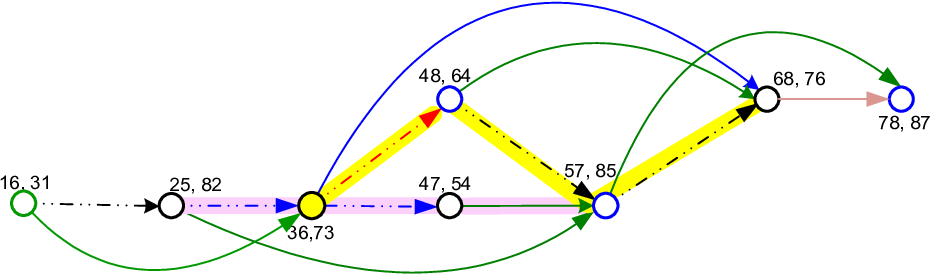
Refer to caption
Figure 9: A Subset of Cโ€‹Vโ€‹Mโ€‹Pโ€‹Sโ€‹eโ€‹tโ€‹(mโ€‹dโ€‹aโ€‹gโ€‹โŸจ(16,31)โŸฉ,mโ€‹dโ€‹aโ€‹gโ€‹โŸจ(57,85)โŸฉ)CV\hskip-2.0ptM\hskip-1.5ptP\hskip-0.5ptSet(mdag\langle(16,31)\rangle,mdag\langle(57,85)\rangle)

Product of two VMPs

Let qโˆˆCโ€‹Vโ€‹Mโ€‹Pโ€‹Sโ€‹eโ€‹tโ€‹(xi+1,xnโˆ’1)q\in CV\hskip-2.0ptM\hskip-1.5ptP\hskip-0.5ptSet(x_{i+1},x_{n-1}) and ฯ€โก(q)\pi(q) be the corresponding permutation in G(i)G^{(i)}, where xiโˆˆgโก(i)x_{i}\in g(i).
Then by xiโˆ™qx_{i}\centerdot q we imply the product ฯ€โก(q)โ€‹ฯˆโ€‹(xi)โˆˆG(iโˆ’1)\pi(q)\psi(x_{i})\in G^{(i-1)}, where xiโˆ™qโˆˆCโ€‹Vโ€‹Mโ€‹Pโ€‹Sโ€‹eโ€‹tโ€‹(xi,xnโˆ’1)x_{i}\centerdot q\in CV\hskip-2.0ptM\hskip-1.5ptP\hskip-0.5ptSet(x_{i},x_{n-1}).

Further, by induction, we can use the term product pโˆ™qp\centerdot q of two adjacent VMPs, (p,q)(p,q), to denote the multiplication of the associated permutations, noting that when p=mโ€‹dโ€‹aโ€‹gโ€‹(xi,xi+1,xi+2)p=mdag(x_{i},x_{i+1},x_{i+2}) it is same as xiโˆ™qx_{i}\centerdot q.

The product of two VMPSetย then can be defined as,

Vโ€‹Mโ€‹Pโ€‹Sโ€‹eโ€‹tโ€‹(mi,mt)โˆ™Vโ€‹Mโ€‹Pโ€‹Sโ€‹eโ€‹tโ€‹(mt,mj)โ€‹=defโ€‹{pโˆ™q|(p,q)โˆˆVโ€‹Mโ€‹Pโ€‹Sโ€‹eโ€‹tโ€‹(mi,mt)ร—Vโ€‹Mโ€‹Pโ€‹Sโ€‹eโ€‹tโ€‹(mt,mj)}\hskip-10.0ptV\hskip-2.0ptM\hskip-1.5ptP\hskip-0.5ptSet(m_{i},m_{t})\centerdot V\hskip-2.0ptM\hskip-1.5ptP\hskip-0.5ptSet(m_{t},m_{j})\overset{\text{def}}{=}\big\{p\centerdot q\,\big|\,(p,q)\in V\hskip-2.0ptM\hskip-1.5ptP\hskip-0.5ptSet(m_{i},m_{t})\times V\hskip-2.0ptM\hskip-1.5ptP\hskip-0.5ptSet(m_{t},m_{j})\big\} (4.2)

Note that again, all qโˆˆVโ€‹Mโ€‹Pโ€‹Sโ€‹eโ€‹tโ€‹(mt,mj)q\in V\hskip-2.0ptM\hskip-1.5ptP\hskip-0.5ptSet(m_{t},m_{j}) cannot be multiplied by all pโˆˆVโ€‹Mโ€‹Pโ€‹Sโ€‹eโ€‹tโ€‹(mi,mt)p\in V\hskip-2.0ptM\hskip-1.5ptP\hskip-0.5ptSet(m_{i},m_{t}).

CVMPSetย Properties

Let xix_{i} be any node in the iith node partition gโก(i)g(i) of the generating graph ฮ“โก(n)\Gamma(n), where 1โ‰คiโ‰คnโˆ’11\leq i\leq n-1. Let ฯˆโก(xi)\psi(x_{i}) and ฯˆโก(yi)\psi(y_{i}) be the two coset representatives in UiU_{i} realized by the nodes xix_{i} and yiy_{i} respectively, where UiU_{i} is the set of coset representatives for the subgroup G(i)<G(iโˆ’1)<SnG^{(i)}<G^{(i-1)}<S_{n}.

Property 4.2.

All CVMP sets, CVMPSet(mdag<xi>,mdag<xnโˆ’1>)CV\hskip-2.0ptM\hskip-1.5ptP\hskip-0.5ptSet(mdag\textless{}x_{i}\textgreater{},~mdag\textless{}x_{n-1}\textgreater{}), are mutually disjoint for each mdag pair (mdag<xi>,mdag<xnโˆ’1>)(mdag\textless{}x_{i}\textgreater{},~mdag\textless{}x_{n-1}\textgreater{}) and each i,1โ‰คiโ‰คnโˆ’2i,~1\leq i\leq n-2.

Proof. Note that each CVMP set, CVMPSet(mdag<xi>,mdag<xnโˆ’1>)CV\hskip-2.0ptM\hskip-1.5ptP\hskip-0.5ptSet(mdag\textless{}x_{i}\textgreater{},mdag\textless{}x_{n-1}\textgreater{}), is uniquely defined by its two mdags. Moreover, every xiโˆˆgโก(i)x_{i}\in g(i) as well as every RR-edge and every mdag at xix_{i} are unique. And therefore, if every CVMP, pโˆˆCVMPSet(mdag<xi>,mdag<xnโˆ’1>)p\in CV\hskip-2.0ptM\hskip-1.5ptP\hskip-0.5ptSet(mdag\textless{}x_{i}\textgreater{},mdag\textless{}x_{n-1}\textgreater{}), is unique, so are all xiโ‹…pโˆˆCโ€‹Vโ€‹Mโ€‹Pโ€‹Sโ€‹eโ€‹tโ€‹(xi,xnโˆ’1)x_{i}\cdot p\in CV\hskip-2.0ptM\hskip-1.5ptP\hskip-0.5ptSet(x_{i},x_{n-1}). That is, for each (xi,yi)โˆˆgโก(i)(x_{i},y_{i})\in g(i) and for each prโˆˆCVMPSet(mdag<xi+1>,mdag<xnโˆ’1>)p_{r}\in CV\hskip-2.0ptM\hskip-1.5ptP\hskip-0.5ptSet(mdag\textless{}x_{i+1}\textgreater{},mdag\textless{}x_{n-1}\textgreater{}),

xi\displaystyle\vskip-9.0ptx_{i} โ‰ yiโŸนxiโ‹…prโ‰ yiโ‹…pr,ย and\displaystyle\neq y_{i}\Longrightarrow x_{i}\cdot p_{r}\neq y_{i}\cdot p_{r},\text{ and}
p1\displaystyle p_{1} โ‰ p2โŸนxiโ‹…p1โ‰ xiโ‹…p2.\displaystyle\neq p_{2}\Longrightarrow x_{i}\cdot p_{1}\neq x_{i}\cdot p_{2}.\text{ \vskip-5.0pt}

And hence, by induction, the disjointness of CVMPSet(mdag<xi>,mdag<xnโˆ’1>)CV\hskip-2.0ptM\hskip-1.5ptP\hskip-0.5ptSet(mdag\textless{}x_{i}\textgreater{},mdag\textless{}x_{n-1}\textgreater{}) follows from the disjointness of the contained CVMPs.

โˆŽ

Property 4.3.

There are at the most Oโก(n5)O(n^{5}) CVMP sets, CVMPSet(mdag<xi>,mdag<xnโˆ’1>)CV\hskip-2.0ptM\hskip-1.5ptP\hskip-0.5ptSet(mdag\textless{}x_{i}\textgreater{},mdag\textless{}x_{n-1}\textgreater{}), between any node pair (xi,xnโˆ’1)(x_{i},x_{n-1}) in a generating graph ฮ“โก(n)\Gamma(n).

Proof. We simply note that there are Oโก(n2)O(n^{2}) nodes xiโˆˆgโก(i)x_{i}\in g(i) at any node partition ii in ฮ“โก(n),aโ€‹nโ€‹d\Gamma(n),andthere are Oโก(n3)O(n^{3}) mdags at each node. Moreover, there are only two nodes in the node partition nโˆ’1n-1.

โˆŽ

4.1.1 Partition of a Coset into CVMPSets

Lemma 4.4.

Each Coset G(i)โ€‹ฯˆkG^{(i)}\psi_{k} of a subgroup G(i)<G(iโˆ’1)G^{(i)}<G^{(i-1)} can be partitioned into a family of equivalence classes, viz., the CVMPSets, as follows:

G(i)โ€‹ฯˆk=โจ„xnโˆ’1,ฯˆโก(ai)=ฯˆkCโ€‹Vโ€‹Mโ€‹Pโ€‹Sโ€‹eโ€‹tโ€‹(mโ€‹dโ€‹aโ€‹gโ€‹โŸจaiโŸฉ,mโ€‹dโ€‹aโ€‹gโ€‹โŸจxnโˆ’1โŸฉ),G^{(i)}\psi_{k}=\biguplus_{\begin{subarray}{c}x_{n-1},\\ \psi(a_{i})=\psi_{k}\end{subarray}}\hskip-10.0ptCV\hskip-2.0ptM\hskip-1.5ptP\hskip-0.5ptSet\!(mdag\langle a_{i}\rangle,mdag\langle x_{n-1}\rangle),\vskip 0.0pt (4.3)

where ฯˆk=(i,k)โˆˆUi\psi_{k}=(i,k)\in U_{i}, aiโˆˆgโก(i),xnโˆ’1โˆˆgโก(nโˆ’1)a_{i}\in g(i),~x_{n-1}\in g(n-1), 1โ‰คi<nโˆ’11\leq i<n-1.

Proof. The proof follows essentially from Property 4.2 and an observation that the multiplication mโ€‹dโ€‹aโ€‹gโ€‹โŸจaiโŸฉโ‹…cโ€‹vโ€‹mโ€‹pmdag\langle a_{i}\rangle\cdot cvmp where cโ€‹vโ€‹mโ€‹pโˆˆCโ€‹Vโ€‹Mโ€‹Pโ€‹Sโ€‹eโ€‹tโ€‹(mโ€‹dโ€‹aโ€‹gโ€‹โŸจaOPENi+1)โŸฉ,mโ€‹dโ€‹aโ€‹gโ€‹โŸจxnโˆ’1โŸฉ)cvmp\in CV\hskip-2.0ptM\hskip-1.5ptP\hskip-0.5ptSet(mdag\langle a_{i+1)}\rangle,mdag\langle x_{n-1}\rangle), defines an equivalence relation over the coset G(i)โ€‹ฯˆkG^{(i)}\psi_{k}.

Clearly, each distinct cvmp in a CVMPSet(mdag<ai+1>,mdag<xnโˆ’1>)CV\hskip-2.0ptM\hskip-1.5ptP\hskip-0.5ptSet(mdag\textless{}a_{i+1}\textgreater{},mdag\textless{}x_{n-1}\textgreater{}) represents a unique permutation ฯ€โˆˆG(i)\pi\in G^{(i)}. By the definition of a CVMPSet we also know that it contains precisely those CVMPs from Cโ€‹Vโ€‹Mโ€‹Pโ€‹Sโ€‹eโ€‹tโ€‹(mโ€‹dโ€‹aโ€‹gโ€‹โŸจai+1โŸฉ,mโ€‹dโ€‹aโ€‹gโ€‹โŸจxnโˆ’1โŸฉ)CV\hskip-2.0ptM\hskip-1.5ptP\hskip-0.5ptSet(mdag\langle a_{i+1}\rangle,mdag\langle x_{n-1}\rangle) which can be multiplied by a common mdag at the node aia_{i}.
Since the set {ai|ฯˆโก(ai)=ฯˆk}\{a_{i}|\psi(a_{i})=\psi_{k}\} represents the coset representative ฯˆkโˆˆUi\psi_{k}\in U_{i}, each CVMP in Cโ€‹Vโ€‹Mโ€‹Pโ€‹Sโ€‹eโ€‹tโ€‹(mโ€‹dโ€‹aโ€‹gโ€‹โŸจaiโŸฉ,mโ€‹dโ€‹aโ€‹gโ€‹โŸจxnโˆ’1โŸฉ)CV\hskip-2.0ptM\hskip-1.5ptP\hskip-0.5ptSet(mdag\langle a_{i}\rangle,mdag\langle x_{n-1}\rangle) represents the product ฯ€โ€‹ฯˆโ€‹(ai)\pi\psi(a_{i}) in the coset G(i)โ€‹ฯˆโ€‹(ai)G^{(i)}\psi(a_{i}).
Therefore, a union of all these (disjoint) subsets satisfying ฯˆโก(ai)=ฯˆk\psi(a_{i})=\psi_{k} gives G(i)โ€‹ฯˆโ€‹(ai)G^{(i)}\psi(a_{i}).

โˆŽ

Note. For each node aiโˆˆgโก(i)a_{i}\in g(i) there are Oโก(n3)O(n^{3}) distinct mโ€‹dโ€‹aโ€‹g<ai>mdag\textless{}a_{i}\textgreater{} over which the above union operation in (4.3) is performed.

4.1.2 Coverage of the Symmetric Group ๐’๐ง\mathbf{S_{n}}

Property 4.5.

All the CVMPSets of length nโˆ’1n\!-\!1 in ฮ“โก(n)\Gamma(n) jointly contain n!n! unique CVMPs representing precisely the n!n! permutations in SnS_{n}. That is,

โจ„a1โˆˆgโก(1),xnโˆ’1โˆˆgโก(nโˆ’1)Cโ€‹Vโ€‹Mโ€‹Pโ€‹Sโ€‹eโ€‹tโ€‹(mโ€‹dโ€‹aโ€‹gโ€‹โŸจa1โŸฉ,mโ€‹dโ€‹aโ€‹gโ€‹โŸจxnโˆ’1โŸฉ)=Sn\biguplus_{\begin{subarray}{c}a_{1}\in g(1),\\ x_{n-1}\in g(n-1)\end{subarray}}\hskip-15.0ptCV\hskip-2.0ptM\hskip-1.5ptP\hskip-0.5ptSet(mdag\langle a_{1}\rangle,mdag\langle x_{n-1}\rangle)=S_{n} (4.4)

Proof. The proof follows from (4.3) of Lemma 4.4.
Note that gโก(1)g(1) is the set of all the edge pairs that collectively represent the generators (elements in the set of right coset representatives), U1U_{1}, and further all the associated CVMP sets are mutually disjoint (Property 4.2).
Therefore,

Sn=โจ„ฯˆkโˆˆU1G(1)โ€‹ฯˆk=โจ„a1โˆˆgโก(1),xnโˆ’1โˆˆgโก(nโˆ’1)Cโ€‹Vโ€‹Mโ€‹Pโ€‹Sโ€‹eโ€‹tโ€‹(mโ€‹dโ€‹aโ€‹gโ€‹โŸจa1โŸฉ,mโ€‹dโ€‹aโ€‹gโ€‹โŸจxnโˆ’1โŸฉ).\displaystyle\begin{split}S_{n}=\biguplus_{\psi_{k}\in U_{1}}G^{(1)}\psi_{k}&=\biguplus_{\begin{subarray}{c}a_{1}\in g(1),\\ x_{n-1}\in g(n-1)\end{subarray}}\hskip-15.0ptCV\hskip-2.0ptM\hskip-1.5ptP\hskip-0.5ptSet(mdag\langle a_{1}\rangle,mdag\langle x_{n-1}\rangle).\end{split}\vskip 0.0pt

โˆŽ

4.1.3 Counting Perfect Matchings in ๐Š๐ง,๐ง\mathbf{K_{n,n}}

To demonstrate the basic counting technique, we first present a counting algorithm that enumerates seemingly a trivial set, viz., the set of all n!n! perfect matchings in Kn,nK_{n,n} in polynomial time. We will then augment the same algorithm to allow the counting in any bipartite graph, while still maintaining the polynomial time bound. The following algorithm describes the high level steps which realize the group enumeration technique as captured by Property 4.4 and 4.5.

Algorithm 4.1 CountAllPerfectMatchings (Kn,nK_{n,n})
โ€‚Input: generating graph ฮ“โก(n)\Gamma(n);
โ€‚Output: count of Prefect Matchings in Kn,nK_{n,n};
ย 
Step (a): Inductively compute all CVMPSets
1: โ€‚for node partitions i=nโˆ’3i=n-3 to 11 do
2: โ€ƒโ€‚for all nodes aiโˆˆgโก(i)a_{i}\in g(i) do
3: โ€ƒโ€ƒโ€‚for all (ai+1,xnโˆ’1)โˆˆgโก(i+1)ร—gโก(nโˆ’1)(a_{i+1},x_{n-1})\in g(i+1)\times g(n-1) do
4: โ€ƒโ€ƒโ€ƒโ€‚compute all Cโ€‹Vโ€‹Mโ€‹Pโ€‹Sโ€‹eโ€‹tโ€‹(mโ€‹dโ€‹aโ€‹gโ€‹โŸจaiโŸฉ,mโ€‹dโ€‹aโ€‹gโ€‹โŸจxnโˆ’1โŸฉ)CV\hskip-2.0ptM\hskip-1.5ptP\hskip-0.5ptSet(mdag\langle a_{i}\rangle,mdag\langle x_{n-1}\rangle) ={mโ€‹dโ€‹aโ€‹gโ€‹โŸจaiโŸฉโ‹…Cโ€‹Vโ€‹Mโ€‹Pโ€‹Sโ€‹eโ€‹tโ€‹(mโ€‹dโ€‹aโ€‹gโ€‹โŸจai+1โŸฉ,mโ€‹dโ€‹aโ€‹gโ€‹โŸจxnโˆ’1โŸฉ)}=\{mdag\langle a_{i}\rangle\cdot CV\hskip-2.0ptM\hskip-1.5ptP\hskip-0.5ptSet(mdag\langle a_{i+1}\rangle,mdag\langle x_{n-1}\rangle)\};
5: โ€ƒโ€ƒโ€‚end for
6: โ€ƒโ€‚end for
7: โ€‚end for
Step (b): Sum the counts in each CVMPSet
tโ€‹hโ€‹eโ€‹Cโ€‹oโ€‹uโ€‹nโ€‹t=โˆ‘(a1,xnโˆ’1)Cโ€‹Vโ€‹Mโ€‹Pโ€‹Sโ€‹eโ€‹tโ€‹(mโ€‹dโ€‹aโ€‹gโ€‹โŸจa1โŸฉ,mโ€‹dโ€‹aโ€‹gโ€‹โŸจxnโˆ’1โŸฉ)โ‹…Cโ€‹oโ€‹uโ€‹nโ€‹t\displaystyle\hskip-180.67499ptthe~Count\,=\,\sum_{(a_{1},\,x_{n-1})}\hskip-10.0ptCV\hskip-2.0ptM\hskip-1.5ptP\hskip-0.5ptSet(mdag\langle a_{1}\rangle,mdag\langle x_{n-1}\rangle)\cdot Count

As we shall see that the most complex step in the above algorithm 4.1 is the step (4), incrementing a Cโ€‹Vโ€‹Mโ€‹Pโ€‹Sโ€‹eโ€‹tโ€‹(mโ€‹dโ€‹aโ€‹gโ€‹โŸจai+1โŸฉ,mโ€‹dโ€‹aโ€‹gโ€‹โŸจxnโˆ’1โŸฉ)CV\hskip-2.0ptM\hskip-1.5ptP\hskip-0.5ptSet(mdag\langle a_{i+1}\rangle,mdag\langle x_{n-1}\rangle) by an mโ€‹dโ€‹aโ€‹gโ€‹โŸจaiโŸฉmdag\langle a_{i}\rangle.

The Disjoint Subsets of CVMP Sets

Unlike the product ฯ€โ€‹ฯˆ\pi\psi in a coset G(1)โ€‹ฯˆG^{(1)}\psi of the group G(1)G^{(1)}, most xiโˆˆgโก(i)x_{i}\in g(i) cannot multiply all the CVMPs in any Cโ€‹Vโ€‹Mโ€‹Pโ€‹Sโ€‹eโ€‹tโ€‹(xi+1,xnโˆ’1)CV\hskip-2.0ptM\hskip-1.5ptP\hskip-0.5ptSet(x_{i+1},x_{n-1}), but only a subset thereof induced by xix_{i}. Therefore, we need to find the disjoint subsets of Cโ€‹Vโ€‹Mโ€‹Pโ€‹Sโ€‹eโ€‹tโ€‹(mi+1,mnโˆ’1)CV\hskip-2.0ptM\hskip-1.5ptP\hskip-0.5ptSet(m_{i+1},m_{n-1}) in which all CVMPs can be multiplied by a common xiโˆˆgโก(i)x_{i}\in g(i). The structure, pโ€‹rโ€‹oโ€‹dโ€‹Vโ€‹Mโ€‹Pโ€‹Sโ€‹eโ€‹tโ€‹(mi,mt,mnโˆ’1)prodV\hskip-2.0ptM\hskip-1.5ptP\hskip-0.5ptSet(m_{i},m_{t},m_{n-1}), defined below is one accomplishes this capability.

Let xrโˆˆgโก(r)x_{r}\in g(r) be node in the node partition ii of ฮ“โก(n)\Gamma(n) for 1โ‰คrโ‰คn1\leq r\leq n; let mr=mdag(<xr>)m_{r}=mdag(\textless{}x_{r}\textgreater{}) denote an mdag at the node xrx_{r}, and let Cโ€‹Vโ€‹Mโ€‹Pโ€‹Sโ€‹eโ€‹tโ€‹(mi,mnโˆ’1)CV\hskip-2.0ptM\hskip-1.5ptP\hskip-0.5ptSet(m_{i},\,m_{n-1}) be any subset of the coset G(i)โ€‹ฯˆkG^{(i)}\psi_{k} in (4.3).

We define pโ€‹rโ€‹oโ€‹dโ€‹Vโ€‹Mโ€‹Pโ€‹Sโ€‹eโ€‹tโ€‹(mi,mt,mnโˆ’1)prodV\hskip-2.0ptM\hskip-1.5ptP\hskip-0.5ptSet(m_{i},m_{t},m_{n-1}) as a family of disjoint subsets of Cโ€‹Vโ€‹Mโ€‹Pโ€‹Sโ€‹eโ€‹tโ€‹(mi,mnโˆ’1)CV\hskip-2.0ptM\hskip-1.5ptP\hskip-0.5ptSet(m_{i},m_{n-1}) as follows.

Definition 4.6.

Let mt=mโ€‹dโ€‹aโ€‹gโ€‹(xt,xt+1,yl)m_{t}=mdag(x_{t},x_{t+1},y_{l}), 1<iโ‰คtโ‰คnโˆ’11<i\leq t\leq n-1. Then

prodVMPSet(mi,mt,mnโˆ’1)=def{pโˆˆCVMPSet(mi,mnโˆ’1)โˆฃpย coversย mtย such thatย the nodeย xt+1ย inย mtย is incident byย R-edges,ย Rxt+1,ย with commonย Sโ€‹Eโ€‹(Rxj+1)}prodV\hskip-2.0ptM\hskip-1.5ptP\hskip-0.5ptSet(m_{i},\,m_{t},\,m_{n-1})\overset{\text{def}}{=}\{p\in CV\hskip-2.0ptM\hskip-1.5ptP\hskip-0.5ptSet(m_{i},\,m_{n-1})\mid\text{$p$ covers $m_{t}$ such that }\\ \text{the node $x_{t+1}$ in $m_{t}$ is incident by $R$-edges, $R_{x_{t+1}}$,}\text{ with common $S\hskip-2.0ptE(R_{x_{j+1}})$\lx@text@rbrace} (4.5)
Refer to caption
Figure 10: ๐ฉ๐ซ๐จ๐๐•๐Œ๐๐’๐ž๐ญโก(๐ฆ๐ข,๐ฆ๐ญ,๐ฆ๐งโˆ’๐Ÿ)\mathbf{prodV\hskip-2.0ptM\hskip-1.5ptP\hskip-0.5ptSet(m_{i},\,m_{t},\,m_{n-1})}: Disjoint Subsets of ๐‚๐•๐Œ๐๐’๐ž๐ญโก(๐ฆ๐ข,๐ฆ๐งโˆ’๐Ÿ)\mathbf{CV\hskip-2.0ptM\hskip-1.5ptP\hskip-0.5ptSet(m_{i},\,m_{n-1})}

Remark. In general a node xt+1x_{t+1} in mtm_{t} covered by pp can have 0 to 2 RR-edges incident upon it. Thus for each mtm_{t}, there are 4 possible disjoint subsets induced by the 2 incident RR-edges.

The following Property follows directly from the above definition.

Property 4.7.

For each fixed t,1โ‰คtโ‰คnโˆ’1t,~1\leq t\leq n-1, the associated disjoint subsets, pโ€‹rโ€‹oโ€‹dโ€‹Vโ€‹Mโ€‹Pโ€‹Sโ€‹eโ€‹tโ€‹(mi,mt,mnโˆ’1)prodV\hskip-2.0ptM\hskip-1.5ptP\hskip-0.5ptSet(m_{i},\,m_{t},\,m_{n-1}), are related to Cโ€‹Vโ€‹Mโ€‹Pโ€‹Sโ€‹eโ€‹tโ€‹(mi,mnโˆ’1)CV\hskip-2.0ptM\hskip-1.5ptP\hskip-0.5ptSet(m_{i},\,m_{n-1}) as follows:

Cโ€‹Vโ€‹Mโ€‹Pโ€‹Sโ€‹eโ€‹tโ€‹(mi,mnโˆ’1)=โจ„mtpโ€‹rโ€‹oโ€‹dโ€‹Vโ€‹Mโ€‹Pโ€‹Sโ€‹eโ€‹tโ€‹(mi,mt,mnโˆ’1)CV\hskip-2.0ptM\hskip-1.5ptP\hskip-0.5ptSet(m_{i},\,m_{n-1})~=~\biguplus_{m_{t}}\hskip-0.1ptprodV\hskip-2.0ptM\hskip-1.5ptP\hskip-0.5ptSet(m_{i},\,m_{t},\,m_{n-1}) (4.6)
Property 4.8.
pโ€‹rโ€‹oโ€‹dโ€‹Vโ€‹Mโ€‹Pโ€‹Sโ€‹eโ€‹tโ€‹(mi,mt,mj)=Vโ€‹Mโ€‹Pโ€‹Sโ€‹eโ€‹tโ€‹(mi,mt)โˆ™Vโ€‹Mโ€‹Pโ€‹Sโ€‹eโ€‹tโ€‹(mt,mj)prodV\hskip-2.0ptM\hskip-1.5ptP\hskip-0.5ptSet(m_{i},\,m_{t},\,m_{j})=V\hskip-2.0ptM\hskip-1.5ptP\hskip-0.5ptSet(m_{i},\,m_{t})\centerdot V\hskip-2.0ptM\hskip-1.5ptP\hskip-0.5ptSet(m_{t},\,m_{j}) (4.7)

Proof. Folllows from the definition of the product of two VMPs in (4.2).

โˆŽ

4.2 Perfect Matching Generators

In this section we develop generators for a subproblem of perfect matchings, the MinSet sequences. This subproblem is an equivalence class of the n!n! perfect matchings, represented as a sequence of a P-time enumerable structure called MinSets which is induced by the missing edges in each potential perfect matching.

We first define MinSets which are collections of VMPs induced by the โ€œmissing" edges, and which in turn are modeled as an attribute called Edge Requirements(ER) of a CVMP that would represent an existing perfect matching under certain conditions on the ER. These MinSets become generators for the MinSet Sequences, and hence for the perfect matchings.

4.2.1 Edge Requirements: the CVMP Qualifier

Edge Requirement is an algebraic formulation of the perfect matching behavior that every node in the graph is incident with exactly one edge, i.e., the matched edge. To define the edge requirement of a CVMP (VMP), pp, we will define two terms, viz. the edge requirement, Eโ€‹Rโ€‹(xi)ER(x_{i}), of a node, xix_{i} in pp, and surplus edge, Sโ€‹Eโ€‹(xtโ€‹xi)SE(x_{t}x_{i}), of an RR-edge xtโ€‹xix_{t}x_{i}.

Let p=x1x2โ‹ฏxnโˆ’1xnp=x_{1}x_{2}\cdots x_{n-1}x_{n} be CVMP in ฮ“โก(n)\Gamma(n) for a bipartite graph Bโ€‹GBG. The (initial) Edge Requirement, Eโ€‹Rโ€‹(xi)ER(x_{i}) of a node xiโˆˆgโก(i)x_{i}\in g(i) in pp is

Eโ€‹Rโ€‹(xi)โ€‹=defโ€‹{e|eโˆˆxiโ€‹ย andย โ€‹eโˆ‰Bโ€‹G}ER(x_{i})\overset{\text{def}}{=}\{e~|~e\in x_{i}~\text{ and }e\notin BG\} (4.8)

xix_{i} represents an initial assignment of the matched edges incident on the node pair (vi,wi)(v_{i},w_{i}).
We first consider the perfect matchings in Kn,nK_{n,n}. There are exactly two ways each node pair (vj,wj)โˆˆKn,n(v_{j},w_{j})\in K_{n,n} can be incident with 2 matched edges in a perfect matching in Kn,nK_{n,n}:

  1. 1.

    The node pair (vj,wj)(v_{j},w_{j}) is incident with an edge pair represented by xjโˆˆgโก(j)x_{j}\in g(j), and

  2. 2.

    one or both the edges in xjx_{j} incident on (vj,wj)(v_{j},w_{j}) are replaced by 2 alternate edges of a cycle formed between xiโˆˆgโก(i)x_{i}\in g(i) and xjx_{j} such that xiโ€‹Rโ€‹xjx_{i}Rx_{j}, where xix_{i} is in pp.

For each instance of an RR-edge xiโ€‹Rโ€‹xjx_{i}Rx_{j} in pp, the edge in the edge-pair xjx_{j} being replaced by the RR-cycle xiโ€‹Rโ€‹xjx_{i}Rx_{j} will be called a Surplus Edge, Sโ€‹Eโ€‹(xiโ€‹xj)SE(x_{i}x_{j}), and is defined as follows:

Sโ€‹Eโ€‹(xiโ€‹xj)โ€‹=defโ€‹ย the edgeย eโˆˆxjย covered by the associatedย R-cycle defined byย xiโ€‹Rโ€‹xj.ย \vskip-5.0ptSE(x_{i}x_{j})\overset{\text{def}}{=}\text{ the edge $e\in x_{j}$ covered by the associated $R$-cycle defined by $x_{i}Rx_{j}$. }\vskip 0.0pt (4.9)

When the given graph is not a complete bipartite graph, the edge requirement of a node xx in ฮ“โก(n)\Gamma(n) can be met by the surplus edge(s) as determined by the RR-edges incident on xx. For example, in Figure 11, for the CVMP p=(12,31)โ‹…(24,32)โ‹…(34,43)โ‹…(44,44)p=(12,31)\cdot(24,32)\cdot(34,43)\cdot(44,44), the initial Eโ€‹RER of various nodes on pp, i.e.,{44,34,32}\{44,34,32\}, is satisfied by the SE of the incident RR-edges.

Refer to caption
Figure 11: A Perfect Matching: satisfying the Edge Requirements

The Edge Requirement Eโ€‹Rโ€‹(p)ER(p) of a VMP, pp in ฮ“โก(n)\Gamma(n), is the collection of each of the nodesโ€™ Edge Requirement that is not satisfied by the SE of the RR-edge incident on that node. That is,

ER(p)=defโ‹ƒxiโˆˆpER(xi)โˆ’({SE(xjxk)|xj,xkโˆˆp}โ‹‚(โ‹ƒxiโˆˆpER(xi)))ER(p)\overset{\text{def}}{=}\bigcup_{x_{i}\in p}ER(x_{i})-\big(\{SE(x_{j}x_{k})~|~x_{j},x_{k}\in p\}\bigcap\big(\bigcup_{x_{i}\in p}ER(x_{i})~\big)~\big)\vskip-10.0pt (4.10)

(The intersection in the second term is needed simply to avoid any โ€œnegative edge requirementsโ€ resulting from any redundant edges incident on any of the nodes.)

As a VMP pp in ฮ“โก(n)\Gamma(n) grows, its edge requirements Eโ€‹Rโ€‹(p)ER(p) can change. We will show later (Lemma 4.10) that the edge requirements of a VMP, pp in ฮ“โก(n)\Gamma(n) is null iff pp leads to a perfect matching in Bโ€‹Gโ€ฒBG^{\prime}. Note that Eโ€‹Rโ€‹(p)ER(p) is specific to a given bipartite graph Bโ€‹Gโ€ฒBG^{\prime} since the ER of a node in pp depends on Bโ€‹Gโ€ฒBG^{\prime}, whereas SE of an RR-edge is fixed for all Bโ€‹Gโ€ฒBG^{\prime}.

The following corollary follows directly from Lemma A.13

Corollary 4.9.

Every Cโ€‹Vโ€‹Mโ€‹P,CV\hskip-2.0ptM\hskip-1.0ptP\!\!, p=x1x2โ‹ฏxnโˆ’1xnp=x_{1}x_{2}~\cdots~x_{n-1}x_{n} in ฮ“โก(n)\Gamma(n), represents a unique perfect matching Eโก(ฯ€)E(\pi) in Kn,nK_{n,n} given by

E(ฯ€)=โ‹ƒxiโˆˆpxiโˆ’{SE(xjxk)โˆฃxjRxk,(xj,xk)โˆˆp}.E(\pi)=\bigcup_{x_{i}\in p}{x_{i}}-\{SE(x_{j}x_{k})\mid x_{j}Rx_{k},\,(x_{j},x_{k})\in p\}. (4.11)

The Condition for a CVMP to be a Perfect Matching

Lemma 4.10.

Let p=x1x2โ‹ฏxnโˆ’1xnp=x_{1}x_{2}~\cdots~x_{n-1}x_{n} be a CVMP of length nโˆ’1n-1 for a bipartite graph Bโ€‹Gโ€ฒBG^{\prime}. Then Eโ€‹Rโ€‹(p)=โˆ…โŸบEโก(ฯ€)ER(p)=\emptyset\Longleftrightarrow E(\pi) is a perfect matching in Bโ€‹Gโ€ฒBG^{\prime} given by (4.11), where ฯ€\pi is given by (3.7).

Proof. The expression for Eโ€‹Rโ€‹(p)ER(p) in (4.10) can be re-written as:

Eโ€‹Rโ€‹(p)=\displaystyle ER(p)= (โ‹ƒxiโˆˆpER(xi))โ‹‚({e|eโˆˆxiโˆˆp}โˆ’{SE(xjxk)|xj,xkโˆˆp}))\displaystyle\big(\bigcup_{x_{i}\in p}ER(x_{i})\big)\bigcap\big(\{e~|~e\in x_{i}\in p\}-\{SE(x_{j}x_{k})~|~x_{j},x_{k}\in p\})~\big)
=\displaystyle= (โ‹ƒxiโˆˆpEโ€‹Rโ€‹(xi))โ€‹โ‹‚Eโก(ฯ€)\displaystyle\big(\bigcup_{x_{i}\in p}ER(x_{i})~\big)\bigcap E(\pi)

Therefore, Eโ€‹Rโ€‹(p)=โˆ…ER(p)=\emptyset iff either
โ€ƒโ€ƒโ€ƒโ€ƒโ€ƒโ€ƒโ€ƒโ€ƒโ€ƒโ€ƒโ€ƒโ€ƒโ€… (1) โˆ€xiโˆˆp,Eโ€‹Rโ€‹(xi)=โˆ…\forall x_{i}\in p,ER(x_{i})=\emptyset, or
โ€ƒโ€ƒโ€ƒโ€ƒโ€ƒโ€ƒโ€ƒโ€ƒโ€ƒโ€ƒโ€ƒโ€ƒโ€… (2) โˆ€eโˆˆEโก(ฯ€),eโˆ‰โˆชEโ€‹Rโ€‹(xi)\forall e\in E(\pi),~e\notin\cup ER(x_{i}), and hence eโˆˆBโ€‹Gโ€ฒe\in BG^{\prime}.

Thus both cases lead to Eโก(ฯ€)E(\pi) being realized by Bโ€‹Gโ€ฒBG^{\prime}.

โˆŽ

A Pattern of ER Satisfiability

Following the enumeration scheme in A.15, each step of constructing incrementally larger length CVMPSetย can reduce the Eโ€‹RER of its member CVMPs by at the most one edge. For example, each perfect matching in Cโ€‹Vโ€‹Mโ€‹Pโ€‹Sโ€‹eโ€‹tโ€‹(m1,mnโˆ’1)CV\hskip-2.0ptM\hskip-1.5ptP\hskip-0.5ptSet(m_{1},m_{n-1}) can allow at the most one missing edge in the perfect matchings in Bโ€‹G1BG_{1} as illustrated in Figure 12 below.

Refer to caption
Figure 12: Incremental Reduction of ER

The following Property is a consequence of Lemma A.15.

Property 4.11.

For every (x1,p2)โˆˆgโก(1)ร—Cโ€‹Vโ€‹Mโ€‹Pโ€‹Sโ€‹eโ€‹tโ€‹(m2,mnโˆ’1)(x_{1},p_{2})\in g(1)\times CV\hskip-2.0ptM\hskip-1.5ptP\hskip-0.5ptSet(m_{2},m_{n-1}), if x1โˆ™p2x_{1}\centerdot p_{2} is a perfect matching in Bโ€‹GBG, then |Eโ€‹Rโ€‹(p2)|โ‰ค1|ER(p_{2})|\leq 1.

Proof. The permutation group enumeration (Lemma A.15) requires that each p2โˆˆCโ€‹Vโ€‹Mโ€‹Pโ€‹Sโ€‹eโ€‹tโ€‹(m2,mnโˆ’1)p_{2}\in CV\hskip-2.0ptM\hskip-1.5ptP\hskip-0.5ptSet(m_{2},m_{n-1}) be multiplied by exactly one generating element x1โˆˆgโก(1)x_{1}\in g(1) in order to generate another member x1โˆ™p2x_{1}\centerdot p_{2} in Cโ€‹Vโ€‹Mโ€‹Pโ€‹Sโ€‹eโ€‹tโ€‹(m1,mnโˆ’1)CV\hskip-2.0ptM\hskip-1.5ptP\hskip-0.5ptSet(m_{1},m_{n-1}).
Therefore, Eโ€‹Rโ€‹(x1โˆ™p2)=โˆ…โŸน|Eโ€‹Rโ€‹(p2)|โ‰ค1ER(x_{1}\centerdot p_{2})=\emptyset\Longrightarrow|ER(p_{2})|\leq 1.

โˆŽ

4.2.2 MinSets: The VMPs of Common ER

Counting all the VMPs of a common ER for any given bipartite graph cannot be done in polynomial time because of the possibility of exponentially many ER sequences over a VMPSet. However, for certain small fixed patterns of the ERs, the VMPSet can be counted in polynomial time.

The above Property 4.11 drives the definition of an ER-constrained set, called MinSet, which has a common ER for all the contained VMPs. A Cโ€‹Vโ€‹Mโ€‹Pโ€‹Sโ€‹eโ€‹tโ€‹(m1,mnโˆ’1)CV\hskip-2.0ptM\hskip-1.5ptP\hskip-0.5ptSet(m_{1},m_{n-1}) can then be expressed as a polynomially bounded set of a sequence of P-time enumerable MinSets.

Let Eโ€‹Rpโ€‹(xj)ER^{p}(x_{j}) denote the ER of a node xjx_{j} covered by a VMP, pp.

Definition 4.12.

A Mโ€‹iโ€‹nโ€‹Sโ€‹eโ€‹tโ€‹(mi,mj)MinSet(m_{i},m_{j}), 1โ‰คi<jโ‰คnโˆ’11\leq i<j\leq n-1, is the largest subset of Vโ€‹Mโ€‹Pโ€‹Sโ€‹eโ€‹tโ€‹(mi,mj)V\hskip-2.0ptM\hskip-1.5ptP\hskip-0.5ptSet(m_{i},\,m_{j}), where each pโˆˆMโ€‹iโ€‹nโ€‹Sโ€‹eโ€‹tโ€‹(mi,mj)p\in MinSet(m_{i},\,m_{j}) has a common ER, Eโ€‹Rโ€‹(p)ER(p), such that

โˆ€(p,xk)โˆˆMโ€‹iโ€‹nโ€‹Sโ€‹eโ€‹tโ€‹(mi,mj)\forall(p,x_{k})\in MinSet(m_{i},\,m_{j}), the common ER, Eโ€‹Rpโ€‹(xk)=โˆ…ER^{p}(x_{k})=\emptyset except for the 3 common nodes, xi,xi+1x_{i},~~x_{i+1}, and xj+1x_{j+1}, in 3 distinguished node partitions (i,i+1i,~{i+1}, and j+1{j+1})
(Fig 13).

Refer to caption
Figure 13: An Abstract MinSet: ๐Œ๐ข๐ง๐’๐ž๐ญ(๐ฆ๐๐š๐ <๐ฑ๐ข>,๐ฆ๐๐š๐ <๐ฑ๐ฃ>)\mathbf{MinSet(mdag\textless{}x_{i}\textgreater{},mdag\textless{}x_{j}\textgreater{})}

Representation of a MinSet

A MinSet has a representation similar to that of a VMPSet except for the additional attributes for the common ER and the incident RR-edges. For notational convenience, the common ER at the 3rd node xj+1x_{j+1} is not being captured, although it can differ between any two MinSet(mdag<xi>,mdag<xj>){MinSet(mdag\textless{}x_{i}\textgreater{},mdag\textless{}x_{j}\textgreater{})}.

Eโ€‹dโ€‹gโ€‹eโ€‹sโ€‹Aโ€‹tโ€‹Nโ€‹oโ€‹dโ€‹eโ€‹(ย Node, {incident edges})EdgesAtNode~(\text{ {Node}, \lx@text@lbrace incident edges\lx@text@rbrace});
Nโ€‹oโ€‹dโ€‹eโ€‹Pโ€‹aโ€‹rโ€‹tโ€‹iโ€‹tโ€‹iโ€‹oโ€‹nโ€‹ย Array[ ]ย ofย โ€‹Eโ€‹dโ€‹gโ€‹eโ€‹sโ€‹Aโ€‹tโ€‹Nโ€‹oโ€‹dโ€‹eNodePartition\text{ {Array}[ ] \emph{of }}EdgesAtNode;

๐Œ๐ข๐ง๐’๐ž๐ญ(๐ฆ๐๐š๐ โŸจ๐š๐ขโŸฉ,๐ฆ๐๐š๐ โŸจ๐›๐ฃโŸฉ)=ย Structย {Mโ€‹dโ€‹aโ€‹gโ€‹Pโ€‹aโ€‹iโ€‹rโ€‹ย (mdag<ai>, ย mdag<bj>);Pโ€‹aโ€‹rโ€‹tโ€‹iโ€‹tโ€‹iโ€‹oโ€‹nโ€‹Lโ€‹iโ€‹sโ€‹tโ€‹Array[iโ‹…โ‹…(j+1)]ย ofโ€‹NodePartition;ย //ER at 3 distinguished node positionsCโ€‹oโ€‹mโ€‹mโ€‹oโ€‹nโ€‹Eโ€‹Rโ€‹Eโ€‹Rโ€‹(xi);Cโ€‹oโ€‹mโ€‹mโ€‹oโ€‹nโ€‹Eโ€‹Rโ€‹Eโ€‹Rโ€‹(xi+1);Cโ€‹oโ€‹mโ€‹mโ€‹oโ€‹nโ€‹Eโ€‹Rโ€‹Eโ€‹Rโ€‹(xj+1);Cโ€‹oโ€‹uโ€‹nโ€‹tโ€‹integer;// the count of all the contained VMPs}\vskip-8.0pt\begin{split}\mathbf{MinSet(mdag\langle a_{i}\rangle,~mdag\langle b_{j}\rangle)=}\textbf{ Struct }\{\\ &MdagPair\text{ (mdag\textless{}$a_{i}$\textgreater{}, ~mdag\textless{}$b_{j}$\textgreater{});}\\ &PartitionList~\text{{Array}[$i\,\cdot\cdot\,(j\!+\!1)$]\, \emph{{of}}}\,\text{NodePartition;}\\ &\text{ //ER at 3 distinguished node positions}\\ &CommonER~ER(x_{i});~~\\ &CommonER~ER(x_{i+1});~\\ &CommonER~ER(x_{j+1});~\\ &Count~\textbf{integer};\text{// the count of all the contained VMPs}\\ &\}\end{split}\vskip-18.0pt (4.12)
Definition 4.13.

A Mโ€‹iโ€‹nโ€‹Sโ€‹eโ€‹tโ€‹(mi,mt,mj)MinSet(m_{i},m_{t},m_{j}), 1โ‰คi<jโ‰คnโˆ’11\leq i<j\leq n-1, is a distinguished Mโ€‹iโ€‹nโ€‹Sโ€‹eโ€‹tโ€‹(mi,mj)MinSet(m_{i},m_{j}) such that
โ€ƒโ€ƒโ€‚โ€„(1) Mโ€‹iโ€‹nโ€‹Sโ€‹eโ€‹tโ€‹(mi,mt,mj)โІpโ€‹rโ€‹oโ€‹dโ€‹Vโ€‹Mโ€‹Pโ€‹Sโ€‹eโ€‹tโ€‹(mi,mt,mj)MinSet(m_{i},m_{t},m_{j})\subseteq prodV\hskip-2.0ptM\hskip-1.5ptP\hskip-0.5ptSet(m_{i},\,m_{t},\,m_{j}), and
โ€ƒโ€ƒโ€‚โ€„(2) Eโ€‹Rโ€‹(mt)=Eโ€‹Rโ€‹(xt+1)ER(m_{t})=ER(x_{t+1}), where mt=mโ€‹dโ€‹aโ€‹gโ€‹(xt,xt+1,xr)m_{t}=mdag(x_{t},x_{t+1},x_{r}).

Fact 4.14.

For Kn,nK_{n,n},

Cโ€‹Vโ€‹Mโ€‹Pโ€‹Sโ€‹eโ€‹tโ€‹(mi,mnโˆ’1)=Mโ€‹iโ€‹nโ€‹Sโ€‹eโ€‹tโ€‹(mi,mnโˆ’1).CV\hskip-2.0ptM\hskip-1.5ptP\hskip-0.5ptSet(m_{i},m_{n-1})=MinSet(m_{i},m_{n-1}).

Notation: The labeling of nodes and edges in ฮ“โก(n)\Gamma(n)

Assuming the nodes in Kn,nK_{n,n} are labeled from NN using decimal numbers, a node (iโ€‹v,wโ€‹i)โˆˆฮ“โก(n)(iv,wi)\in\Gamma(n) is then labeled as i.v,w.ii.v,w.i, while the RR-edges ((iโ€‹v,wโ€‹i),(wโ€‹v,tโ€‹w))((iv,wi),(wv,tw)) are labled by +w.v+w.v, where `โ€‹`โ‹…"``\cdot" is used as a delimiter to separate the node labels. When the node numbers are 0,1,2,โ‹ฏโ€‰90,1,2,\,\cdots\,9, we will ignore this delimiter `โ€‹`โ‹…"``\cdot".

4.2.3 Finding the MinSets of a CVMPSet

We begin with an example CVMPSet,โ€‰ showing how do the various MinSets compose a CVMPSet. We show how a MinSet is determined for the various values of ERs of x4x_{4} and x6x_{6} in the subset of a Cโ€‹Vโ€‹Mโ€‹Pโ€‹Sโ€‹eโ€‹tโ€‹(m1,m5)CV\hskip-2.0ptM\hskip-1.5ptP\hskip-0.5ptSet(m_{1},m_{5}) in a bipartite graph. We consider two cases: a) when Eโ€‹Rโ€‹(x6)={68}ER(x_{6})=\{68\}, and b) when Eโ€‹Rโ€‹(x4)={48},Eโ€‹Rโ€‹(x6)={68}ER(x_{4})=\{48\},ER(x_{6})=\{68\}.

Refer to caption
Figure 14: A CVMPSet Subset with 2 CVMPs

VMPSet Partition 1: Eโ€‹Rโ€‹(x6)={68}ER(x_{6})=\{68\}

Here the two MinSets differ in the common RR-edge incident at x6x_{6}.

Cโ€‹Vโ€‹Mโ€‹Pโ€‹Sโ€‹eโ€‹tโ€‹(m1,m5)=Mโ€‹iโ€‹nโ€‹Sโ€‹eโ€‹tโ€‹(m1,m5)+Mโ€‹iโ€‹nโ€‹Sโ€‹eโ€‹tโ€‹(m1,m5โ€ฒ)CV\hskip-2.0ptM\hskip-1.5ptP\hskip-0.5ptSet(m_{1},m_{5})=MinSet(m_{1},m_{5})+MinSet(m_{1},m^{\prime}_{5})

[Uncaptioned image]

VMPSet Partition 2: Eโ€‹Rโ€‹(x4)={48},Eโ€‹Rโ€‹(x6)={68}ER(x_{4})=\{48\},ER(x_{6})=\{68\}

Vโ€‹Mโ€‹Pโ€‹Sโ€‹eโ€‹tโ€‹(m1,m5)=Mโ€‹iโ€‹nโ€‹Sโ€‹eโ€‹tโ€‹(m1,m3)โˆ™Mโ€‹iโ€‹nโ€‹Sโ€‹eโ€‹tโ€‹(m3,m5)+Mโ€‹iโ€‹nโ€‹Sโ€‹eโ€‹tโ€‹(m1,m5)V\hskip-2.0ptM\hskip-1.5ptP\hskip-0.5ptSet(m_{1},m_{5})=\!MinSet(m_{1},m_{3})\centerdot MinSet(m_{3},m_{5})+MinSet(m_{1},m_{5})

[Uncaptioned image]
Lemma 4.15.

For each Vโ€‹Mโ€‹Pโ€‹Sโ€‹eโ€‹tโ€‹(mr,ms)V\hskip-2.0ptM\hskip-1.5ptP\hskip-0.5ptSet(m_{r},m_{s}) there are at the most 4 MinSets, Mโ€‹iโ€‹nโ€‹Sโ€‹eโ€‹tโ€‹(mr,ms)MinSet(m_{r},m_{s}).

Proof. By Definition 4.13, for a fixed (mr,ms)(m_{r},m_{s}), two MinSets in {Mโ€‹iโ€‹nโ€‹Sโ€‹eโ€‹tโ€‹(mr,ms)}\{MinSet(m_{r},m_{s})\} can differ only due to 3rd distinguished node because of the incident RR-edges can make its ER to be different. For any other node at positions {r+2,r+3,โ‹ฏs}\{r+2,r+3,\cdots~s\}, a non-null ER would imply MinSets of shorter length.
Moreover, the first two nodes do not have any RR-edges incident on them. Thus, the 3rd node is the only one left that can induce subsets of Vโ€‹Mโ€‹Pโ€‹Sโ€‹eโ€‹tโ€‹(mr,ms)V\hskip-2.0ptM\hskip-1.5ptP\hskip-0.5ptSet(m_{r},m_{s}) due to its two possible ERs resulting from the incident RR-edges.

Now the ER of this 3rd distinguished node, Eโ€‹Rโ€‹(xs+1)ER(x_{s+1}), can take at the most 4 values corresponding to the 4 possible subsets of the edge pair xs+1โˆˆgโก(s+1)x_{s+1}\in g(s+1) in msm_{s}. Therefore, for any fixed (mr,ms)(m_{r},m_{s}),

|{Mโ€‹iโ€‹nโ€‹Sโ€‹eโ€‹tโ€‹(mr,ms)}|โ‰ค4\big|\{MinSet(m_{r},m_{s})\}\big|~\leq~4\vskip-15.0pt

.

โˆŽ

Remark. Clearly, any Vโ€‹Mโ€‹Pโ€‹Sโ€‹eโ€‹tโ€‹(mr,ms)V\hskip-2.0ptM\hskip-1.5ptP\hskip-0.5ptSet(m_{r},m_{s}) of length more than 3 can have an empty MinSet, Mโ€‹iโ€‹nโ€‹Sโ€‹eโ€‹tโ€‹(mr,ms)MinSet(m_{r},m_{s}), because of the non null edge requirements.

Lemma 4.16.

The maximum number of Mโ€‹iโ€‹nโ€‹Sโ€‹eโ€‹tโ€‹(mi,mt,mnโˆ’1)MinSet(m_{i},m_{t},m_{n-1}), 1โ‰คiโ‰คtโ‰คnโˆ’11\leq i\leq t\leq n-1, for a given Cโ€‹Vโ€‹Mโ€‹Pโ€‹Sโ€‹eโ€‹tโ€‹(mi,mnโˆ’1)CV\hskip-2.0ptM\hskip-1.5ptP\hskip-0.5ptSet(m_{i},m_{n-1}) is bounded by Oโก(n6)O(n^{6}).

Proof. The bound follows from the bound on the maximum number of mdags covered by any Cโ€‹Vโ€‹Mโ€‹Pโ€‹Sโ€‹eโ€‹tโ€‹(mi,mnโˆ’1)CV\hskip-2.0ptM\hskip-1.5ptP\hskip-0.5ptSet(m_{i},m_{n-1}) in a given node partition, where there can be Oโก(n3)O(n^{3}) mdags, mโ€‹dโ€‹aโ€‹g<xi>mdag\textless{}x_{i}\textgreater{} at any node xix_{i}.

โˆŽ

4.2.4 The Structure of a CVMPSetย Partition

We will now show the exact composition of a CVMPSetย  in terms of its components, the MinSets.

The Covering MinSet- a subset of CVMPSet

Now we show how each Cโ€‹Vโ€‹Mโ€‹Pโ€‹Sโ€‹eโ€‹tโ€‹(mi,mnโˆ’1)CV\hskip-2.0ptM\hskip-1.5ptP\hskip-0.5ptSet(m_{i},m_{n-1}) can be partitioned into disjoint subsets which are equivalence classes represented by a sequence of MinSets. We first define this MinSet sequence and then show how does it cover a Cโ€‹Vโ€‹Mโ€‹Pโ€‹Sโ€‹eโ€‹tโ€‹(mi,mnโˆ’1)CV\hskip-2.0ptM\hskip-1.5ptP\hskip-0.5ptSet(m_{i},m_{n-1}).

Refer to caption
Figure 15: Sequences of 1-2 MinSets:

Cโ€‹Vโ€‹Mโ€‹Pโ€‹Sโ€‹eโ€‹tโ€‹(mi,mnโˆ’1)=โจ„Mโ€‹iโ€‹nโ€‹Sโ€‹eโ€‹tโ€‹(mi,mt)โˆ™Mโ€‹iโ€‹nโ€‹Sโ€‹eโ€‹tโ€‹(mt,mnโˆ’1)CV\hskip-2.0ptM\hskip-1.5ptP\hskip-0.5ptSet(m_{i},m_{n-1})=\biguplus MinSet(m_{i},m_{t})\centerdot MinSet(m_{t},m_{n-1})

Let โˆ\prod denote the product of two or more adjacent MinSets, similar to the product of VMPSets.

Definition 4.17.

A covering minset, Cโ€‹Mโ€‹Siโ€‹tโ€‹(r)CMS_{it}(r), represents a subset of Vโ€‹Mโ€‹Pโ€‹Sโ€‹eโ€‹tโ€‹(mi,mt)V\hskip-2.0ptM\hskip-1.5ptP\hskip-0.5ptSet(m_{i},m_{t}) by a sequence of rr MinSets for the given Vโ€‹Mโ€‹Pโ€‹Sโ€‹eโ€‹tโ€‹(mi,mt)V\hskip-2.0ptM\hskip-1.5ptP\hskip-0.5ptSet(m_{i},m_{t}).

That is,

Cโ€‹Mโ€‹Siโ€‹tโ€‹(r)โ€‹=defโ€‹{Mโ€‹iโ€‹nโ€‹Sโ€‹eโ€‹tโ€‹(mi,mj1),Mโ€‹iโ€‹nโ€‹Sโ€‹eโ€‹tโ€‹(mj1,mj2),โ‹ฏ,Mโ€‹iโ€‹nโ€‹Sโ€‹eโ€‹tโ€‹(mjrโˆ’1,mt)},CMS_{it}(r)\overset{\text{def}}{=}\{MinSet(m_{i},m_{j_{1}}),MinSet(m_{j_{1}},m_{j_{2}}),~\cdots,~MinSet(m_{j_{r-1}},m_{t})\},

such that

โˆijโˆˆIMโ€‹iโ€‹nโ€‹Sโ€‹eโ€‹tโ€‹(mij,mij+1)โІVโ€‹Mโ€‹Pโ€‹Sโ€‹eโ€‹tโ€‹(mi,mt),\prod_{i_{j}\in I}MinSet(m_{i_{j}},m_{i_{j+1}})~\subseteq V\hskip-2.0ptM\hskip-1.5ptP\hskip-0.5ptSet(m_{i},m_{t}),

where I={i,j1,j2,โ‹ฏ,jrโˆ’1}I=\{i,j_{1},j_{2},\cdots,~j_{r-1}\} is an index set representing the various node partitions induced by the Eโ€‹Rโ‰ โˆ…ER\neq\emptyset nodes in Vโ€‹Mโ€‹Pโ€‹Sโ€‹eโ€‹tโ€‹(mi,mt)V\hskip-2.0ptM\hskip-1.5ptP\hskip-0.5ptSet(m_{i},m_{t}) such that |I|=r|I|=r, 1โ‰คrโ‰คtโˆ’i1\leq r\leq t-i.

The following Lemma 4.18 precisely states the composition of a Cโ€‹Vโ€‹Mโ€‹Pโ€‹Sโ€‹eโ€‹tโ€‹(mi,mnโˆ’1)CV\hskip-2.0ptM\hskip-1.5ptP\hskip-0.5ptSet(m_{i},m_{n-1}) in terms of its MinSet sequences.

Lemma 4.18.

Let Cโ€‹Mโ€‹Siโ€‹nโ€‹(r)CMS_{in}(r) be a MinSet sequence of length rr representing a subset of Cโ€‹Vโ€‹Mโ€‹Pโ€‹Sโ€‹eโ€‹tโ€‹(mi,mnโˆ’1)CV\hskip-2.0ptM\hskip-1.5ptP\hskip-0.5ptSet(m_{i},m_{n-1}), where 1โ‰คrโ‰คnโˆ’21\leq r\leq n-2, 1โ‰คiโ‰คnโˆ’21\leq i\leq n-2.
Further, let I={i,r1,r2,โ‹ฏ,nโˆ’1}I=\{i,r_{1},r_{2},\cdots,~n-1\} be an index set representing the indices to various node partitions induced by the Eโ€‹Rโ‰ โˆ…ER\neq\emptyset nodes in Cโ€‹Mโ€‹Siโ€‹nโ€‹(r)CMS_{in}(r) such that |I|=1+r|I|=1+r. Then, for all i,1โ‰คiโ‰คnโˆ’2i,1\leq i\leq n-2,

Cโ€‹Vโ€‹Mโ€‹Pโ€‹Sโ€‹eโ€‹tโ€‹(mi,mnโˆ’1)=โจ„r=1nโˆ’2โˆCโ€‹Mโ€‹Siโ€‹nโ€‹(r),ijโˆˆIMโ€‹iโ€‹nโ€‹Sโ€‹eโ€‹tโ€‹(mij,mij+1)CV\hskip-2.0ptM\hskip-1.5ptP\hskip-0.5ptSet(m_{i},m_{n-1})=\biguplus_{\hskip-1.0ptr=1}^{n-2}\hskip 0.0pt\prod_{\hskip 3.0pt\begin{subarray}{c}C\hskip-1.0ptM\hskip-1.0ptS\,\hskip-2.0pt_{in}(r),\\ i_{j}\in I\end{subarray}}\hskip-15.0ptMinSet(m_{i_{j}},m_{i_{j+1}})\vskip-5.0pt (4.13)

(The proof is deferred until after the counting algorithm)

The Equivalence Class- MinSet Sequences

We define a new equivalence class induced by the following equivalence relation โ„œ\mathbb{\mathbf{\Re}} over the
set CVMPSet.

The Equivalence Relation โ„œ\mathbb{\mathbf{\Re}}

Definition 4.19.
โˆ€(pi,pj)โˆˆCโ€‹Vโ€‹Mโ€‹Pโ€‹Sโ€‹eโ€‹tโ€‹(mi,mnโˆ’1),piโ€‹โ„œโกpjโŸบ\displaystyle\vskip-20.0pt\forall(p_{i},p_{j})\in CV\hskip-2.0ptM\hskip-1.5ptP\hskip-0.5ptSet(m_{i},m_{n-1}),~p_{i}\mathbb{\mathbf{\Re}}p_{j}\Longleftrightarrow โˆƒย a prefixย Mโ€‹iโ€‹nโ€‹Sโ€‹eโ€‹tโ€‹(mi,mt)ย common to the\displaystyle~\exists\text{ a prefix $MinSet(m_{i},m_{t})$ common to the }
sequences in (4.13) containingย piย andย pj.\displaystyle\text{ sequences in \eqref{EQ:CMS-partition} containing $p_{i}$ and $p_{j}$}.
Claim 4.20.

The relation โ„œ\mathbb{\mathbf{\Re}} is an equivalence relation over the set CVMPSet((mi,mnโˆ’1)๐ถ๐ฟ๐‘‚๐‘†๐ธ((m_{i},m_{n-1}).

Proof. Follows from Property 4.21.

โˆŽ

Property 4.21.

Every MinSet sequence Cโ€‹Mโ€‹Siโ€‹nโ€‹(r)CMS_{in}(r) in Cโ€‹Vโ€‹Mโ€‹Pโ€‹Sโ€‹eโ€‹tโ€‹(mi,mnโˆ’1)CV\hskip-2.0ptM\hskip-1.5ptP\hskip-0.5ptSet(m_{i},m_{n-1}) is unique.

Proof. Note that each mdag in the mdag sequence {mij,mij+1,โ‹ฏ,mr}\{m_{i_{j}},m_{i_{j+1}},\cdots,m_{r}\} induced by the nodes with Eโ€‹Rโ‰ โˆ…ER\neq\emptyset is unique because of the uniqueness of the missing edges in the bipartite graph.
Now one can view each MinSet sequence, Cโ€‹Mโ€‹Siโ€‹nโ€‹(r)CMS_{in}(r), as words composed out of unique mdags with Eโ€‹Rโ‰ โˆ…ER\neq\emptyset, and without repetitions.
Thus, two MinSet sequences are identical iff the two sequences of the โ€œdelimiting" mdags are identical. Hence each sequence of unique mdags gives rise to a unique sequence in Cโ€‹Mโ€‹Siโ€‹nโ€‹(r)CMS_{in}(r).

โˆŽ

Property 4.22.

There are Oโก(n6)O(n^{6}) prefix MinSets, Mโ€‹iโ€‹nโ€‹Sโ€‹eโ€‹tโ€‹(mi,mt)MinSet(m_{i},m_{t}), for any Cโ€‹Vโ€‹Mโ€‹Pโ€‹Sโ€‹eโ€‹tโ€‹(mi,mnโˆ’1)CV\hskip-2.0ptM\hskip-1.5ptP\hskip-0.5ptSet(m_{i},m_{n-1}), covering all the exponentially many MinSet sequences in (4.13), where 1โ‰คi<tโ‰คnโˆ’11\leq i<t\leq n-1, .

Proof. Note that for each fixed mdag mi,i<tโ‰คnโˆ’1m_{i},~i<t\leq n-1, |{(mi,mt)โˆฃi<tโ‰คnโˆ’1}|=Oโก(n6)|\{(m_{i},m_{t})\mid i<t\leq n-1\}|=O(n^{6}),
and |{Mโ€‹iโ€‹nโ€‹Sโ€‹eโ€‹tโ€‹(mi,mt)}|=cโ€‹|{Vโ€‹Mโ€‹Pโ€‹Sโ€‹eโ€‹tโ€‹(mi,mt)}|,cโ‰ค4|\{MinSet(m_{i},m_{t})\}|=c|\{V\hskip-2.0ptM\hskip-1.5ptP\hskip-0.5ptSet(m_{i},m_{t})\}|,~c\leq 4 (Lemma 4.15).

โˆŽ

Partitions Induced by the MinSet Prefixes

The following Lemma is another version of (4.13) representing a CVMPSetย  partition induced by the prefix MinSets.
Let Pโ€‹Fโ€‹Iโ€‹Xโ€‹(l)PFIX(l) denote a class of MinSets, Mโ€‹iโ€‹nโ€‹Sโ€‹eโ€‹tโ€‹(m1,ml)MinSet(m_{1},m_{l}), containing VMPs of length ll. Also, we define all MinSet sequences of zero length , Cโ€‹Mโ€‹Sโ€‹(0)CMS(0), to be an identity, II, such that

Pโ€‹Fโ€‹Iโ€‹Xโ€‹(l)โˆ™โˆCโ€‹Mโ€‹Sโ€‹(0)Mโ€‹iโ€‹nโ€‹Sโ€‹eโ€‹tโ€‹(mij,mij+1)=Pโ€‹Fโ€‹Iโ€‹Xโ€‹(l).PFIX(l)\centerdot\hskip-10.0pt\prod_{\hskip 3.0ptCMS(0)}\hskip-10.0ptMinSet(m_{i_{j}},m_{i_{j+1}})=PFIX(l).
Lemma 4.23.

Each Cโ€‹Vโ€‹Mโ€‹Pโ€‹Sโ€‹eโ€‹tโ€‹(m1,mnโˆ’1)CV\hskip-2.0ptM\hskip-1.5ptP\hskip-0.5ptSet(m_{1},m_{n-1}) for a bipartite graph can be partitioned into Oโก(n6)O(n^{6}) equivalence classes induced by the Oโก(n6)O(n^{6}) prefix MinSets, Pโ€‹Fโ€‹Iโ€‹Xโ€‹(l)PFIX(l), 2โ‰คlโ‰คnโˆ’12\leq l\leq n-1 in (4.13), such that:

Cโ€‹Vโ€‹Mโ€‹Pโ€‹Sโ€‹eโ€‹tโ€‹(m1,mnโˆ’1)=โจ„l=2nโˆ’1(โจ„r=1nโˆ’lโˆ’1Pโ€‹Fโ€‹Iโ€‹Xโ€‹(l)โˆ™โˆCโ€‹Mโ€‹Siโ€‹nโ€‹(r),l=ijโˆˆIsrโˆ’1Mโ€‹iโ€‹nโ€‹Sโ€‹eโ€‹tโ€‹(mij,mij+1)),CV\hskip-2.0ptM\hskip-1.5ptP\hskip-0.5ptSet(m_{1},m_{n-1})=\biguplus_{l=2}^{n-1}\Bigl(\biguplus_{\hskip-1.0ptr=1}^{n-l-1}\hskip 0.0ptPFIX(l)\centerdot\hskip-7.0pt\prod_{\hskip 3.0pt\begin{subarray}{c}C\hskip-1.0ptM\hskip-1.0ptS\,\hskip-2.0pt_{in}(r),\\ {l=i_{j}\in I}\end{subarray}}^{s_{r-1}}\hskip-15.0ptMinSet(m_{i_{j}},m_{i_{j+1}})\Bigr),\vskip-5.0pt (4.14)

where ll, 2โ‰คlโ‰คnโˆ’12\leq l\leq n-1, is the first index in any index set, I={1,s1=l,s2,โ‹ฏ,srโˆ’1,nโˆ’1}I=\{1,s_{1}\!=\!l,s_{2},\cdots,s_{r-1},n-1\}, representing all the node partitions induced by the Eโ€‹Rโ‰ โˆ…ER\neq\emptyset nodes in Cโ€‹Mโ€‹Siโ€‹nโ€‹(r)CMS_{in}(r).

Proof. The proof follows from Lemma 4.18, Property 4.21 and Property 4.22.

โˆŽ

The following figures ([Fig 16 and Fig 17]) depict the partition implied by (4.14), i.e., how Oโก(n6)O(n^{6}) prefix MinSets induce polynomially many (Oโก(n6)O(n^{6})) equivalence classes containing exponentially many Cโ€‹Mโ€‹Siโ€‹nโ€‹(r)CMS_{in}(r) sequences in Cโ€‹Vโ€‹Mโ€‹Pโ€‹Sโ€‹eโ€‹tโ€‹(mi,mnโˆ’1)CV\hskip-2.0ptM\hskip-1.5ptP\hskip-0.5ptSet(m_{i},m_{n-1}).

Refer to caption
Figure 16: CVMP Set Partitions by Cโ€‹Mโ€‹Sโ€‹(r)CMS(r) Sequences
Refer to caption
Figure 17: Partition of a CVMPSet Induced by the MinSet Prefixes

A Generating Set for the MinSet Sequences

Before we can describe the counting algorithm, we need one more generating set to consolidate the generation of all the MinSets shared by the various CVMPSets through their CMS partitions. To accomplish this we define a generating set, called Gโ€‹Mโ€‹SG\hskip-1.0ptM\hskip-1.0ptS\,, for generating the Covering MinSets which constitute a partition of CVMPSet.

Definition 4.24.

A generating set for MinSet sequences, Gโ€‹Mโ€‹Sโ€‹(i,n),1โ‰คiโ‰คnโˆ’2G\hskip-1.0ptM\hskip-1.0ptS\,(i,n),~1\leq i\leq n-2, for a bipartite graph on 2โ€‹n2n nodes is a set of MinSets defined as

GMS(i,n)=def{MinSet(mr,ms)|(r,s)โˆˆ[iโ‹…โ‹…nโˆ’2]ร—[i+1โ‹…โ‹…nโˆ’1],r<s},G\hskip-1.0ptM\hskip-1.0ptS\,(i,n)\overset{\text{def}}{=}\big\{MinSet(m_{r},m_{s})\,\big|\,(r,s)\in[i\!\,\cdot\cdot~n\!-\!2]\times[i+1\,\cdot\cdot~n\!-\!1],~r<s\big\},

where {(mr,ms)}\{(m_{r},m_{s})\} covers gโก(r)ร—gโก(s)g(r)\times g(s).

Note that Gโ€‹Mโ€‹Sโ€‹(i,n)G\hskip-1.0ptM\hskip-1.0ptS\,(i,n) contains all the Oโก(n11)O(n^{11}) MinSet prefixes for exponentially many sequences, Cโ€‹Mโ€‹Siโ€‹nโ€‹(r)CMS_{in}(r), for all Cโ€‹Vโ€‹Mโ€‹Pโ€‹Sโ€‹eโ€‹tโ€‹(mi,mnโˆ’1)CV\hskip-2.0ptM\hskip-1.5ptP\hskip-0.5ptSet(m_{i},m_{n-1}) in ฮ“โก(n)\Gamma(n).

The following two properties follow from the definitions of GMSโ€‰and CMS.

Property 4.25.
Gโ€‹Mโ€‹Sโ€‹(1,n)\displaystyle G\hskip-1.0ptM\hskip-1.0ptS\,(1,n)~ โЇโ‹ƒr,(m1,mnโˆ’1)Cโ€‹Mโ€‹S1โ€‹nโ€‹(r)\displaystyle\supseteq\hskip-10.0pt\bigcup_{r,(m_{1},m_{n-1})}\hskip-15.0ptCMS_{1n}(r) (4.15)
Property 4.26.

An upper bound on the size of Gโ€‹Mโ€‹Sโ€‹(1,n)G\hskip-1.0ptM\hskip-1.0ptS\,(1,n) is Oโก(n12)O(n^{12}).

Proof. Note that Gโ€‹Mโ€‹Sโ€‹(1,n)G\hskip-1.0ptM\hskip-1.0ptS\,(1,n) is precisely the set of all the Mโ€‹iโ€‹nโ€‹Sโ€‹eโ€‹tโ€‹(mr,ms)MinSet(m_{r},m_{s}) which connect the Oโก(n12)O(n^{12}) pair of mdags, {(mr,ms)}\{(m_{r},m_{s})\}, by all the VMPs in {Vโ€‹Mโ€‹Pโ€‹Sโ€‹eโ€‹tโ€‹(mr,ms)}\{V\hskip-2.0ptM\hskip-1.5ptP\hskip-0.5ptSet(m_{r},m_{s})\} in ฮ“โก(n)\Gamma(n), where (r,s)โˆˆ[1โ‹…โ‹…nโˆ’2]ร—[r+1โ‹…โ‹…nโˆ’1](r,s)\in[1~\cdot\cdot~n-2]\times[r+1~\cdot\cdot~n-1].
Thus, this bound is same as the bound on the number of edges in a graph with Oโก(n6)O(n^{6}) nodes.
Therefore, by Lemma 4.15,

|Gโ€‹Mโ€‹Sโ€‹(1,n)|โ‰ค4โ€‹|{Vโ€‹Mโ€‹Pโ€‹Sโ€‹eโ€‹tโ€‹(mr,ms)}|โ‰คOโก(n12).\big|G\hskip-1.0ptM\hskip-1.0ptS\,(1,n)\big|\leq 4\big|\{V\hskip-2.0ptM\hskip-1.5ptP\hskip-0.5ptSet(m_{r},m_{s})\}\big|\leq O(n^{12}).\vskip-10.0pt

โˆŽ

5 A Polynomial Time Enumeration Algorithm

Based on the concepts of MinSet sequences developed in the previous Section, we have the following enumeration Algorithm 5.1 which counts all the perfect matchings in a given bipartite graph Bโ€‹GBG on 2โ€‹n2n nodes, nโ‰ฅ3n\geq 3.

Algorithm 5.1 countPerfectMatchings(Bโ€‹G)(BG)
โ€‚Input: a bipartite graph Bโ€‹GBG on 2โ€‹n2n nodes, nโ‰ฅ3n\geq 3;
โ€‚Output: count of the perfect matchings in Bโ€‹GBG;
ย 
Step 0: Initialize- Compute the Initial Generating Set of all the MinSet Sequences


1: โ€‚i=nโˆ’3i=n-3; //ย  ii is the current node partition;
2: โ€‚Compute the generating set EM={gโก(r)โˆฃโ€‰1โ‰คrโ‰คn}E_{M}=\{g(r)\,\mid\,1\leq r\leq n\};
3: โ€‚Compute the generating set Gโ€‹Mโ€‹Sโ€‹(i+1,n)={Mโ€‹iโ€‹nโ€‹Sโ€‹eโ€‹tโ€‹(mnโˆ’2,mnโˆ’1)}G\hskip-1.0ptM\hskip-1.0ptS\,(i+1,n)=\{MinSet(m_{n-2},m_{n-1})\}; //ย the set of all the MinSet Sequences; each Cโ€‹Vโ€‹Mโ€‹Pโ€‹Sโ€‹eโ€‹tโ€‹(mnโˆ’2,mnโˆ’1)CV\hskip-2.0ptM\hskip-1.5ptP\hskip-0.5ptSet(m_{n-2},m_{n-1}) is a Mโ€‹iโ€‹nโ€‹Sโ€‹eโ€‹tโˆˆGโ€‹Mโ€‹Sโ€‹(nโˆ’2,n)MinSet\in G\hskip-1.0ptM\hskip-1.0ptS\,(n\!-\!2,n), with a total count of 6 CVMPs.
ย 
Step 1: Count


โ€ƒโ€ƒโ€‚if (i=0)(i=0) then /โ€‹/ Gโ€‹Mโ€‹Sโ€‹(1,n)G\hskip-1.0ptM\hskip-1.0ptS\,(1,n) may contain the set {Mโ€‹iโ€‹nโ€‹Sโ€‹eโ€‹tโ€‹(m1,mnโˆ’1)}\{MinSet(m_{1},\,m_{n-1})\}

perfect matchingย countย =โˆ‘Eโ€‹R=โˆ…,(m1,mnโˆ’1)Mโ€‹iโ€‹nโ€‹Sโ€‹eโ€‹tโ€‹(m1,mnโˆ’1)โˆ™Cโ€‹oโ€‹uโ€‹nโ€‹t;\vskip-5.0pt\hskip-21.68121pt\text{perfect matching \emph{count} }=\hskip-10.0pt\sum_{\begin{subarray}{c}ER=\emptyset,\\ (m_{1},\,m_{n-1})\end{subarray}}\hskip-15.0ptMinSet(m_{1},\,m_{n-1})\centerdot Count;\ \\ \vskip-1.0pt\vskip-15.0pt

return;
โ€ƒโ€ƒโ€ƒโ€ƒโ€‚โ€„

Step 2: Increment & Join the MinSet Sequences


โ€ƒโ€ƒโ€ƒโ€ƒโ€ƒโ€ƒโ€ƒโ€ƒโ€ƒโ€ƒโ€ƒโ€ƒโ€Šโ€ƒโ€ƒโ€‚iโ€‹nโ€‹cโ€‹rโ€‹eโ€‹mโ€‹eโ€‹nโ€‹tโ€‹Mโ€‹Sโ€‹Sโ€‹(Gโ€‹Mโ€‹Sโ€‹(i+1,n))incrementMSS(G\hskip-1.0ptM\hskip-1.0ptS\,(i\!+\!1,n)); /โ€‹/ assuming nโ‰ฅ3n\geq 3
โ€ƒโ€ƒโ€ƒโ€ƒโ€‚โ€„(Follows the structures in Figure 17)
decrement ii;

repeat Steps 1-2;

End.

5.1 The Polynomial Time Bound

Claim 5.1.

The time complexity of Algorithm 5.1 is Oโก(n45โ€‹logโกn)O(n^{45}\log n).

Proof. Although a tight upper bound would require more details of the algorithm, a fairly loose upper bound should be easy to establish as follows. Let Tโก(oโ€‹pโ€‹s)T(ops) denote the time complexity of the operation oโ€‹pโ€‹sops.

We note that Step 2 calls Algorithm 5.2, iโ€‹nโ€‹cโ€‹rโ€‹eโ€‹mโ€‹eโ€‹nโ€‹tโ€‹Mโ€‹Sโ€‹Sโ€‹()incrementMSS(), having a time complexity Oโก(n44โ€‹logโกn)O(n^{44}\log n), and dominates:

Tโก(Sโ€‹tโ€‹eโ€‹pโ€‹2:โ€‹Iโ€‹nโ€‹cโ€‹rโ€‹eโ€‹mโ€‹eโ€‹nโ€‹t)=Oโก(n44โ€‹logโกn)T(Step~2:\emph{Increment})=O(n^{44}\log n)
Tโก(Sโ€‹tโ€‹eโ€‹pโ€‹1:โ€‹Cโ€‹oโ€‹uโ€‹nโ€‹t)=Oโก(n8)T(Step~1:\emph{Count})=O(n^{8}).

Steps 1-2 are iterated Oโก(n)O(n) times, and thus the time complexity of the counting algorithm
is Oโก(n45โ€‹logโกn)O(n^{45}\log n).

โˆŽ

5.2 Correctness of the Count

Lemma 5.2.

All the perfect matchings in a bipartite graph Bโ€‹GBG on 2โ€‹n2n nodes can be correctly enumerated by 5.1 in polynomial sequential time Oโก(n45โ€‹logโกn)O(n^{45}\log n).

Proof. The correctness of the count follows from the Lemmas 4.18 and 5.4 which prove the following two assertions:

  1. 1.

    All Mโ€‹iโ€‹nโ€‹Sโ€‹eโ€‹tโ€‹(m1,mnโˆ’1)MinSet(m_{1},\,m_{n-1}) with Eโ€‹R=โˆ…ER=\emptyset are contained in Gโ€‹Mโ€‹Sโ€‹(1,n)G\hskip-1.0ptM\hskip-1.0ptS\,(1,n).

  2. 2.

    The perfect matching count is:

    โˆ‘Eโ€‹R=โˆ…,(m1,mnโˆ’1)Mโ€‹iโ€‹nโ€‹Sโ€‹eโ€‹tโ€‹(m1,mnโˆ’1)โˆ™Cโ€‹oโ€‹uโ€‹nโ€‹t\sum_{\begin{subarray}{c}ER=\emptyset,\\ (m_{1},m_{n-1})\end{subarray}}\hskip-10.0ptMinSet(m_{1},m_{n-1})\centerdot Count

โˆŽ

Proof. (of Lemma 4.18)
The proof is by induction on the length rr of the MinSet sequence, Cโ€‹Mโ€‹Siโ€‹nโ€‹(r)CMS_{in}(r). We will consider VMPSets as a general representation of CVMPSets.
Let mj=mโ€‹dโ€‹aโ€‹gโ€‹(xj,xj+1,xd)m_{j}=mdag(x_{j},x_{j+1},x_{d}), where xjโˆˆgโก(j),xj+1โˆˆgโก(j+1)x_{j}\in g(j),x_{j+1}\in g(j+1), and xdโˆˆgโก(d)x_{d}\in g(d).

Case: r=1r=1
The length of a Mโ€‹iโ€‹nโ€‹Sโ€‹eโ€‹tMinSet sequence for a Vโ€‹Mโ€‹Pโ€‹Sโ€‹eโ€‹tโ€‹(mr,ms)V\hskip-2.0ptM\hskip-1.5ptP\hskip-0.5ptSet(m_{r},m_{s}) is one when all the VMPs in the MinSet are of the same length as those in Vโ€‹Mโ€‹Pโ€‹Sโ€‹eโ€‹tโ€‹(mr,ms)V\hskip-2.0ptM\hskip-1.5ptP\hskip-0.5ptSet(m_{r},m_{s}). This can happen when the Eโ€‹Rโ‰ โˆ…ER\neq\emptyset only at the 3 allowed nodes, viz., at xix_{i} or at xi+1x_{i+1} in mim_{i} and xj+1x_{j+1} in mjm_{j}. And then, we have 2 sub cases, that is,
either

Vโ€‹Mโ€‹Pโ€‹Sโ€‹eโ€‹tโ€‹(mi,mj)=Mโ€‹iโ€‹nโ€‹Sโ€‹eโ€‹tโ€‹(mi,mj),ย whenย Eโ€‹Rโ‰ โˆ…ย atย xiย or atย xi+1,V\hskip-2.0ptM\hskip-1.5ptP\hskip-0.5ptSet(m_{i},m_{j})=MinSet(m_{i},m_{j}),\text{ when $ER\neq\emptyset$ at $x_{i}$ or at $x_{i+1}$,} (5.1a)
or
Vโ€‹Mโ€‹Pโ€‹Sโ€‹eโ€‹tโ€‹(mi,mj)=โจ„mjMโ€‹iโ€‹nโ€‹Sโ€‹eโ€‹tโ€‹(mi,mj)=โจ„mjpโ€‹rโ€‹oโ€‹dโ€‹Vโ€‹Mโ€‹Pโ€‹Sโ€‹eโ€‹tโ€‹(mi,mj,mj),V\hskip-2.0ptM\hskip-1.5ptP\hskip-0.5ptSet(m_{i},m_{j})=\biguplus_{m_{j}}MinSet(m_{i},m_{j})=\biguplus_{m_{j}}~prodV\hskip-2.0ptM\hskip-1.5ptP\hskip-0.5ptSet(m_{i},\,m_{j},\,m_{j}),\vskip-5.0pt (5.1b)
when Eโ€‹Rโ€‹(xj+1)โ‰ โˆ…ER(x_{j+1})\neq\emptyset for some pโˆˆVโ€‹Mโ€‹Pโ€‹Sโ€‹eโ€‹tโ€‹(mi,mj)p\in V\hskip-2.0ptM\hskip-1.5ptP\hskip-0.5ptSet(m_{i},m_{j}) at the last node xj+1x_{j+1} in mjm_{j}.

Case: rโ‰ค2r\leq 2

Let Cโ€‹Mโ€‹Siโ€‹jโ€‹(r)={Mโ€‹iโ€‹nโ€‹Sโ€‹eโ€‹tโ€‹(mi,mt),Mโ€‹iโ€‹nโ€‹Sโ€‹eโ€‹tโ€‹(mt,mj)}C\hskip-1.0ptM\hskip-1.0ptS\,_{ij}(r)=\{MinSet(m_{i},m_{t}),MinSet(m_{t},m_{j})\}, where the two MinSets have a common mtm_{t} with Eโ€‹Rโ€‹(mt)โ‰ โˆ…ER(m_{t})\neq\emptyset, i<t<ji<t<j. Then, the first MinSet could be a subset of Vโ€‹Mโ€‹Pโ€‹Sโ€‹eโ€‹tโ€‹(mi,mt)V\hskip-2.0ptM\hskip-1.5ptP\hskip-0.5ptSet(m_{i},\,m_{t}), governed by (5.1b), whereas the second MinSet is the corresponding Vโ€‹Mโ€‹Pโ€‹Sโ€‹eโ€‹tโ€‹(mt,mj)V\hskip-2.0ptM\hskip-1.5ptP\hskip-0.5ptSet(m_{t},m_{j}) by (5.1a).
Therefore, for each such sequence we can apply the result of r=1r=1 to each MinSet and Property 4.7, (4.7) to obtain:

Mโ€‹iโ€‹nโ€‹Sโ€‹eโ€‹tโ€‹(mi,mt)โˆ™Mโ€‹iโ€‹nโ€‹Sโ€‹eโ€‹tโ€‹(mt,mj)\displaystyle MinSet(m_{i},m_{t})\centerdot MinSet(m_{t},m_{j}) โІVโ€‹Mโ€‹Pโ€‹Sโ€‹eโ€‹tโ€‹(mi,mt)โˆ™Vโ€‹Mโ€‹Pโ€‹Sโ€‹eโ€‹tโ€‹(mt,mj)\displaystyle\subseteq V\hskip-2.0ptM\hskip-1.5ptP\hskip-0.5ptSet(m_{i},\,m_{t})\centerdot V\hskip-2.0ptM\hskip-1.5ptP\hskip-0.5ptSet(m_{t},\,m_{j})
=pโ€‹rโ€‹oโ€‹dโ€‹Vโ€‹Mโ€‹Pโ€‹Sโ€‹eโ€‹tโ€‹(mi,mt,mj)\displaystyle=prodV\hskip-2.0ptM\hskip-1.5ptP\hskip-0.5ptSet(m_{i},\,m_{t},\,m_{j})\vskip-5.0pt

Further we note that each mtm_{t} in each sequence of 2 MinSets must be disjoint with each other, irrespective of the node partition tt to which mtm_{t} belongs. Or else, we will have r>2r>2 because of the additional Eโ€‹Rโ‰ โˆ…ER\neq\emptyset nodes common to the same MinSet.
Therefore,

โจ„mtMโ€‹iโ€‹nโ€‹Sโ€‹eโ€‹tโ€‹(mi,mt)โˆ™Mโ€‹iโ€‹nโ€‹Sโ€‹eโ€‹tโ€‹(mt,mj)\displaystyle\biguplus_{m_{t}}MinSet(m_{i},m_{t})\centerdot MinSet(m_{t},m_{j}) =โจ„tโจ„mtpโ€‹rโ€‹oโ€‹dโ€‹Vโ€‹Mโ€‹Pโ€‹Sโ€‹eโ€‹tโ€‹(mi,mt,mj)\displaystyle=\biguplus_{t}\biguplus_{m_{t}}prodV\hskip-2.0ptM\hskip-1.5ptP\hskip-0.5ptSet(m_{i},\,m_{t},\,m_{j})
=Vโ€‹Mโ€‹Pโ€‹Sโ€‹eโ€‹tโ€‹(mi,mj).\displaystyle=V\hskip-2.0ptM\hskip-1.5ptP\hskip-0.5ptSet(m_{i},m_{j}).\vskip-10.0pt

Induction: Sequence size l=r+1l=r+1

If the induction hypothesis is true for all sequence sizes, lโ‰คrl\leq r, then each sequence of length r+1r+1 can be partitioned into 2 subsequences, Mโ€‹iโ€‹nโ€‹Sโ€‹eโ€‹tโ€‹(mi,mt)MinSet(m_{i},m_{t}) and Mโ€‹iโ€‹nโ€‹Sโ€‹eโ€‹tโ€‹(mt,mnโˆ’1)MinSet(m_{t},m_{n-1}), each of length less than or equal to rr.
Therefore, again applying the above cases for rโ‰ค2r\leq 2 we have

Cโ€‹Vโ€‹Mโ€‹Pโ€‹Sโ€‹eโ€‹tโ€‹(mi,mnโˆ’1)=โจ„mtMโ€‹iโ€‹nโ€‹Sโ€‹eโ€‹tโ€‹(mi,mt)โˆ™Mโ€‹iโ€‹nโ€‹Sโ€‹eโ€‹tโ€‹(mt,mnโˆ’1).\vskip-10.0ptCV\hskip-2.0ptM\hskip-1.5ptP\hskip-0.5ptSet(m_{i},m_{n-1})=\biguplus_{m_{t}}MinSet(m_{i},m_{t})\centerdot MinSet(m_{t},m_{n-1}).

โˆŽ

5.3 Examples- Incrementing and Joining the Adjacent MinSets

The following series of figures illustrate the Step 2: โ€œIncrement all the MinSet Sequences" of Algorithm 5.1. Figure 18 shows a bipartite graph with 3 perfect matchings and the associated CVMPs that will generate the perfect matchings. Figure 19 shows a very simple Increment & Join operation on the MinSets.

Refer to caption
Figure 18: A Bipartite Graph and its CVMPs

Figure 19(a) shows two MinSets each having a common Eโ€‹R={8.10}ER=\{8.10\} because of the missing edge (8,10)(8,10) in the bipartite graph.
Figure 19(b) shows an increment of the MinSet1 by x2=(2.10,8.2)x_{2}=(2.10,8.2). This increment creates a jump RR-edge between x2x_{2} and x8x_{8}, and thus satisfying the Eโ€‹R={8.10}ER=\{8.10\} of x8x_{8}, and joining the two MinSets to produce p=Mโ€‹iโ€‹nโ€‹Sโ€‹eโ€‹tโ€‹1โ‹…Mโ€‹iโ€‹nโ€‹Sโ€‹eโ€‹tโ€‹2p=MinSet1\cdot MinSet2, which contains 3 CVMPs. Note that Eโ€‹Rโ€‹(p)=โˆ…ER(p)=\emptyset.
Figure 19(c) shows a further increment of the CVMPs in pp by x1=(1.4,6.1)x_{1}=(1.4,6.1). This gives a set of 3 CVMPs with null ER to produce 3 perfect matchings.

Note: The edge (4,6)(4,6) in the bipartite graph Bโ€‹GBG is not needed for the resulting 3 perfect matchings but its presence simplifies the Step 2 of the algorithm.

Refer to caption
Figure 19: A Simple Increment & Join of 2 MinSets

5.4 The Basic Behavior of Incrementing a MinSet Sequence

The incrementing process can become more intricate if there are other MinSets, Mโ€‹iโ€‹nโ€‹Sโ€‹eโ€‹tโ€‹(mt,ms)MinSet(m_{t},m_{s}), adjacent to Mโ€‹iโ€‹nโ€‹Sโ€‹eโ€‹tโ€‹(mi+1,mt)MinSet(m_{i+1},m_{t}), which may also have to be joined with the prefix MinSet. A simplified view of this process is illustrated in the following Figures 20(a-c). These Figures show how a sequence of three adjacent MinSets is incremented and joined by the multiplying mdags at node partitions, i=2i=2 and i=1i=1.

Figure 20(a) shows a sequence of three MinSets, Mโ€‹S1MS_{1}, Mโ€‹S2MS_{2} and Mโ€‹S3MS_{3}.
Figure 20(b) shows that x2=(2.9,8.2)x_{2}=(2.9,8.2) increments the prefix MinSet, Mโ€‹S1MS_{1} but with no join operation.
Figure 20(c) shows that x1=(1.6,5.1)x_{1}=(1.6,5.1) increments the prefix MinSet, Mโ€‹S1MS_{1} and joins all three MinSets in the sequence.

Refer to caption
Figure 20: Incrementing & Joining the Adjacent MinSets

5.5 Incrementing the MinSet Sequences in ๐†๐Œ๐’\mathbf{G\hskip-1.0ptM\hskip-1.0ptS\,}

The above counting algorithm 5.1 calls the following algorithm 5.2, iโ€‹nโ€‹cโ€‹rโ€‹eโ€‹mโ€‹eโ€‹nโ€‹tโ€‹Mโ€‹Sโ€‹Sโ€‹()incrementM\!SS(), to increment all the MinSet Sequences in Gโ€‹Mโ€‹Sโ€‹(i,n)G\hskip-1.0ptM\hskip-1.0ptS\,(i,n). This algorithm uses two basic operations on MinSet, viz., increment a prefix MinSet, and join two or more adjacent MinSets into one, described by the associated algorithms in the next subsection.

Algorithm 5.2 iโ€‹nโ€‹cโ€‹rโ€‹eโ€‹mโ€‹eโ€‹nโ€‹tโ€‹Mโ€‹Sโ€‹Sโ€‹(Gโ€‹Mโ€‹Sโ€‹(i+1,n))incrementM\!S\!S(G\hskip-1.0ptM\hskip-1.0ptS\,(i+1,n))
โ€‚Input: Gโ€‹Mโ€‹Sโ€‹(i+1,n)G\hskip-1.0ptM\hskip-1.0ptS\,(i+1,n);// contains all sequences Cโ€‹Mโ€‹Si+1,nโ€‹(r),1โ‰คrโ‰คnโˆ’2CMS_{i+1,n}(r),1\leq r\leq n-2
โ€‚Output: Gโ€‹Mโ€‹Sโ€‹(i,n)G\hskip-1.0ptM\hskip-1.0ptS\,(i,n);
ย 
Step (a): Increment all Prefix MinSets, Mโ€‹iโ€‹nโ€‹Sโ€‹eโ€‹tโ€‹(mi+1,ms)โˆˆโ‹ƒCโ€‹Mโ€‹Si+1,nโ€‹(r)MinSet(m_{i+1},m_{s})\in\bigcup CMS_{i+1,n}(r)
1: โ€‚for all xiโˆˆgโก(i)x_{i}\in g(i) do
2: โ€ƒโ€‚for all sโˆˆ[i+2โ‹…โ‹…nโˆ’1],xiRxt+1,s>t+1s\in[i\!+\!2~\cdot\cdot~n\!-\!1],~x_{i}Rx_{t+1},s>t+1 do
3: โ€ƒโ€ƒโ€‚for all Mโ€‹iโ€‹nโ€‹Sโ€‹eโ€‹tโ€‹(mi+1,ms)โˆˆโ‹ƒCโ€‹Mโ€‹Si+1,nโ€‹(r)MinSet(m_{i+1},m_{s})\in\bigcup CMS_{i+1,n}(r) do //ย Oโก(n6)O(n^{6}) MinSets covers all Cโ€‹Mโ€‹Siโ€‹nโ€‹(r)CMS_{in}(r)
4: โ€ƒโ€ƒโ€ƒโ€‚add incrMinSet(mdag<xi>,MinSet(mi+1,ms))incrMinSet(mdag\textless{}x_{i}\textgreater{},MinSet(m_{i+1},m_{s})) to Gโ€‹Mโ€‹Sโ€‹(i,n)G\hskip-1.0ptM\hskip-1.0ptS\,(i,n);
5: โ€ƒโ€ƒโ€‚end for
6: โ€ƒโ€‚end for
7: โ€‚end for
Step (b): Join all the Sub Sequences Selected by Mโ€‹iโ€‹nโ€‹Sโ€‹eโ€‹tโ€‹(mi,mt)MinSet(m_{i},m_{t});


mi=mโ€‹dโ€‹aโ€‹g<xi>,m_{i}=mdag\textless{}x_{i}\textgreater{}, mt=mโ€‹dโ€‹aโ€‹g<xt>,xiโ€‹Rโ€‹xt+1m_{t}=mdag\textless{}x_{t}\textgreater{},~x_{i}Rx_{t+1}.

1: โ€‚for all xiโˆˆgโก(i)x_{i}\in g(i) do
2: โ€ƒโ€‚for all Mโ€‹iโ€‹nโ€‹Sโ€‹eโ€‹tโ€‹(mi,mt)โˆˆGโ€‹Mโ€‹Sโ€‹(i,n)MinSet(m_{i},m_{t})\in G\hskip-1.0ptM\hskip-1.0ptS\,(i,n) do
3: โ€ƒโ€ƒโ€‚uโ€‹pโ€‹dโ€‹aโ€‹tโ€‹eโ€‹Sโ€‹eโ€‹qโ€‹uโ€‹eโ€‹nโ€‹cโ€‹eโ€‹(Mโ€‹iโ€‹nโ€‹Sโ€‹eโ€‹tโ€‹(mi,mt),Gโ€‹Mโ€‹Sโ€‹(i,n))updateSequence(MinSet(m_{i},m_{t}),G\hskip-1.0ptM\hskip-1.0ptS\,(i,n));
4: โ€ƒโ€‚end for
5: โ€‚end for
6: โ€‚return Gโ€‹Mโ€‹Sโ€‹(i,n)G\hskip-1.0ptM\hskip-1.0ptS\,(i,n);

5.5.1 The Time Complexity

Claim 5.3.

The time complexity of Algorithm 5.2 is Oโก(n44โ€‹logโกn)O(n^{44}\log n).

Proof. It should be easy to see that the time in Step(b) dominates.

The For loop at line b(1) is iterated Oโก(n2)O(n^{2}) times, and the For loop at line b(2) is iterated Oโก(n6)O(n^{6}) times determined by the cardinality of {(mi,mt)}\{(m_{i},m_{t})\} for a given xix_{i}.
The time complexity at line b(3) of uโ€‹pโ€‹dโ€‹aโ€‹tโ€‹eโ€‹Sโ€‹eโ€‹qโ€‹uโ€‹eโ€‹nโ€‹cโ€‹eโ€‹()updateSequence() is Oโก(n36โ€‹logโกn)O(n^{36}\log n) (Claim 5.7, Algorithm 5.5).

Therefore, the time complexity of the algorithm as determined by the Step(b) is

Tโก(Sโ€‹tโ€‹eโ€‹pโ€‹(b))=Oโก(n8โˆ—n36โ€‹logโ€‹n)=Oโก(n44โ€‹logโ€‹n)T(Step(b))=O(n^{8}*n^{36}\log n)=O(n^{44}\log n)

.

โˆŽ

5.5.2 Correctness of Algorithm 5.2: incrementMSS()

Lemma 5.4.

For each xiโˆˆgโก(i),iโ‰ฅ1x_{i}\in g(i),i\geq 1 the Algorithm 5.2 increments Gโ€‹Mโ€‹Sโ€‹(i,n)G\hskip-1.0ptM\hskip-1.0ptS\,(i,n) to Gโ€‹Mโ€‹Sโ€‹(iโˆ’1,n)G\hskip-1.0ptM\hskip-1.0ptS\,(i-1,n) to satisfy (4.13) of Lemma 4.18.

Proof.

The correctness follows from the fact that each increment operation by xiโˆˆgโก(i)x_{i}\in g(i) applies either to a prefix or a subset of that prefix to each sequence of MinSets in Gโ€‹Mโ€‹Sโ€‹(i,n)G\hskip-1.0ptM\hskip-1.0ptS\,(i,n). Moreover, all the Oโก(n6)O(n^{6}) prefixes are incremented by the elements xiโˆˆgโก(i)x_{i}\in g(i).

Let pโ€‹s=Mโ€‹iโ€‹nโ€‹Sโ€‹eโ€‹tโ€‹(mi+1,mt)ps=MinSet(m_{i+1},m_{t}) be a prefix to a sequence in Gโ€‹Mโ€‹Sโ€‹(i,n),i+1<tโ‰คnโˆ’2G\hskip-1.0ptM\hskip-1.0ptS\,(i,n),i+1<t\leq n-2, and it is incremented by a unique xiโˆˆgโก(i)x_{i}\in g(i) in Step(a:4). Then, either xiโ‹…pโ€‹sx_{i}\cdot ps is in a MinSet in Gโ€‹Mโ€‹Sโ€‹(iโˆ’1,n)G\hskip-1.0ptM\hskip-1.0ptS\,(i-1,n), or it exists as a new sequence of MinSets in Gโ€‹Mโ€‹Sโ€‹(iโˆ’1,n)G\hskip-1.0ptM\hskip-1.0ptS\,(i-1,n), with a new prefix MinSet for the original MinSet sequence.

Further, when increments by xix_{i} leads to selecting a subset of a MinSet sequence, such a subset of that sequence will also be a valid subset in Vโ€‹Mโ€‹Pโ€‹Sโ€‹eโ€‹tโ€‹(mi,mnโˆ’1)V\hskip-2.0ptM\hskip-1.5ptP\hskip-0.5ptSet(m_{i},m_{n-1}). Hence (4.13) of Lemma 4.18 is always satisfied.

โˆŽ

5.6 Algorithm: Increment a MinSet

Increment of a MinSet, Mโ€‹iโ€‹nโ€‹Sโ€‹eโ€‹tโ€‹(mi+1,ms)MinSet(m_{i+1},m_{s}) by an adjacent mdag, mโ€‹dโ€‹aโ€‹g<xi>mdag\textless{}x_{i}\textgreater{} would involve same kind of operations as in the case of Vโ€‹Mโ€‹Pโ€‹Sโ€‹eโ€‹tโ€‹(mi+1,ms)V\hskip-2.0ptM\hskip-1.5ptP\hskip-0.5ptSet(m_{i+1},m_{s}). Unless the RR-edge from xix_{i} is incident at the two distinguished nodes xi+1x_{i+1} or at xi+2x_{i+2}, the multiplication would cover only a subset of VMPs in Mโ€‹iโ€‹nโ€‹Sโ€‹eโ€‹tโ€‹(mi+1,ms)MinSet(m_{i+1},m_{s}). This subset is determined by the node partition tt in which the node xtx_{t} in Mโ€‹iโ€‹nโ€‹Sโ€‹eโ€‹tโ€‹(mi+1,ms)MinSet(m_{i+1},m_{s}) lies while xiโ€‹Rโ€‹xtx_{i}Rx_{t} holds true.

Refer to caption
Figure 21: Special Case: Incrementing a MinSet at a Common Node xi+1x_{i+1}
Refer to caption
Figure 22: Two Successive Increments at xi+2x_{i+2} and xi+1x_{i+1}

The Step 0 in the algorithm 5.3 covers special cases, where the multiplying mdag multiplies all the VMPs in the MinSet using a common node (Figure 22). The Steps 1-2 show a general case (Figure 22) where the mdag can multiply only a subset of the VMPs from the original MinSet. This involves effectively re-constructing the whole MinSet by the revised list of the multiplying mdags in each node partition.

Algorithm 5.3 iโ€‹nโ€‹cโ€‹rโ€‹Mโ€‹iโ€‹nโ€‹Sโ€‹eโ€‹tโ€‹(mโ€‹dโ€‹aโ€‹gโ€‹โŸจxiโŸฉ,Mโ€‹iโ€‹nโ€‹Sโ€‹eโ€‹tโ€‹(mi+1,ms))incrMinSet(mdag\langle x_{i}\rangle,MinSet(m_{i+1},m_{s}))
โ€‚Input: mi=mdag(xi,xi+1,xt+1),mi+1=mdag(xi+1,xi+2,xt+r),rโ‰ฅ1;MinSet(mi+1,ms)m_{i}=mdag(x_{i},x_{i+1},x_{t+1}),~m_{i+1}=mdag(x_{i+1},x_{i+2},x_{t+r}),r\geq 1;~MinSet(m_{i+1},m_{s})
โ€‚Output: Mโ€‹iโ€‹nโ€‹Sโ€‹eโ€‹tโ€‹(mi,ms)MinSet(m_{i},m_{s}) or {Mโ€‹iโ€‹nโ€‹Sโ€‹eโ€‹tโ€‹(mi,mi+1),Mโ€‹iโ€‹nโ€‹Sโ€‹eโ€‹tโ€‹(mi+1,ms)}\{MinSet(m_{i},m_{i+1}),\,MinSet(m_{i+1},m_{s})\} ย 
Step 0: Initialization and Special Cases
1: โ€‚let xiโ€‹Rโ€‹xt+1x_{i}Rx_{t+1}; given mi+1=mโ€‹dโ€‹aโ€‹gโ€‹(xi+1,xi+2,xt+1)m_{i+1}=mdag(x_{i+1},x_{i+2},x_{t+1});
2: โ€‚if Eโ€‹Rโ€‹(xi+2)โ‰ โˆ…ER(x_{i+2})\neq\emptyset then
3: โ€ƒโ€‚return {Mโ€‹iโ€‹nโ€‹Sโ€‹eโ€‹tโ€‹(mi,mi+1),Mโ€‹iโ€‹nโ€‹Sโ€‹eโ€‹tโ€‹(mi+1,ms)}\{MinSet(m_{i},m_{i+1}),~MinSet(m_{i+1},m_{s})\};
4: โ€‚end if
5: โ€‚if (xiโ€‹Rโ€‹xi+1x_{i}Rx_{i+1} OR xiโ€‹Rโ€‹xi+2x_{i}Rx_{i+2}) then
6: โ€ƒโ€‚return Mโ€‹iโ€‹nโ€‹Sโ€‹eโ€‹tโ€‹(mi,ms)=miโ‹…Mโ€‹iโ€‹nโ€‹Sโ€‹eโ€‹tโ€‹(mi+1,ms)MinSet(m_{i},m_{s})=m_{i}\cdot MinSet(m_{i+1},m_{s});
7: โ€‚end if
ย 
Step 1: Determine the candidate mdags in each node partition of Mโ€‹iโ€‹nโ€‹Sโ€‹eโ€‹tโ€‹(mi+1,ms)MinSet(m_{i+1},m_{s});

assumption: i<tโ‰คsi<t\leq s;

1: โ€‚for all nodePartitionjโˆˆ[i+1โ‹…โ‹…sโˆ’1]nodePartition~j\in[i+1\,\cdot\cdot~s-1] do
2: โ€ƒโ€‚mโ€‹dโ€‹aโ€‹gโ€‹Lโ€‹iโ€‹sโ€‹tโ€‹[j]={mโ€‹dโ€‹aโ€‹gโ€‹โŸจxjโŸฉ}mdagList[j]=\{mdag\langle x_{j}\rangle\};
3: โ€‚end for
4: โ€‚remove each mโ€‹dโ€‹aโ€‹gโ€‹(xt,xt+1,xr)mdag(x_{t},x_{t+1},x_{r}) from mโ€‹dโ€‹aโ€‹gโ€‹Lโ€‹iโ€‹sโ€‹tโ€‹[t]mdagList[t] where xiโ€‹R/xt+1x_{i}{R\hskip-7.0pt\mathbf{/}}\hskip 2.0ptx_{t+1};
ย 
Step 2: Rebuild the whole MinSet with the updated mdags


(sequentially Increment the vmpSets by the mdag List)

1: โ€‚vโ€‹mโ€‹pโ€‹Sโ€‹eโ€‹tโ€‹Lโ€‹iโ€‹sโ€‹t={mโ€‹dโ€‹aโ€‹gโ€‹โŸจxsโˆ’1โŸฉโ‹…ms}vmpSetList=\{mdag\langle x_{s-1}\rangle\cdot m_{s}\};
2: โ€‚for all nโ€‹oโ€‹dโ€‹eโ€‹Pโ€‹aโ€‹rโ€‹tโ€‹iโ€‹tโ€‹iโ€‹oโ€‹nโ€‹j=sโˆ’2โ€‹dโ€‹oโ€‹wโ€‹nโ€‹tโ€‹oโ€‹inodePartition~j=s-2~downto~i do
3: โ€ƒโ€‚for all mโ€‹dโ€‹aโ€‹gโˆˆmโ€‹dโ€‹aโ€‹gโ€‹Lโ€‹iโ€‹sโ€‹tโ€‹[j]mdag\in mdagList[j] do
4: โ€ƒโ€ƒโ€‚nโ€‹eโ€‹wโ€‹Lโ€‹iโ€‹sโ€‹t=โˆ…newList=\emptyset;
5: โ€ƒโ€ƒโ€‚for all vโ€‹mโ€‹pโ€‹Sโ€‹eโ€‹tโˆˆvโ€‹mโ€‹pโ€‹Sโ€‹eโ€‹tโ€‹Lโ€‹iโ€‹sโ€‹tvmpSet\in vmpSetList and adjacent to mโ€‹dโ€‹aโ€‹gmdag do
6: โ€ƒโ€ƒโ€ƒโ€‚update: add mโ€‹dโ€‹aโ€‹gโˆ™vโ€‹mโ€‹pโ€‹Sโ€‹eโ€‹tmdag\centerdot vmpSet to nโ€‹eโ€‹wโ€‹Lโ€‹iโ€‹sโ€‹tnewList;
7: โ€ƒโ€ƒโ€‚end for
8: โ€ƒโ€ƒโ€‚vโ€‹mโ€‹pโ€‹Sโ€‹eโ€‹tโ€‹Lโ€‹iโ€‹sโ€‹tโŸธnโ€‹eโ€‹wโ€‹Lโ€‹iโ€‹sโ€‹tvmpSetList\Longleftarrow newList;
9: โ€ƒโ€‚end for
10: โ€ƒโ€‚if (|mโ€‹dโ€‹aโ€‹gโ€‹Lโ€‹iโ€‹sโ€‹tโ€‹[j]|=1|mdagList[j]|=1) then
11: โ€ƒโ€ƒโ€‚vโ€‹mโ€‹pโ€‹Sโ€‹eโ€‹tโ€‹Lโ€‹iโ€‹sโ€‹tโŸธmโ€‹eโ€‹rโ€‹gโ€‹eโ€‹Mโ€‹iโ€‹nโ€‹Sโ€‹eโ€‹tโ€‹(vโ€‹mโ€‹pโ€‹Sโ€‹eโ€‹tโ€‹Lโ€‹iโ€‹sโ€‹t)vmpSetList\Longleftarrow mergeMinSet(vmpSetList);
12: โ€ƒโ€‚end if
13: โ€‚end for
14: โ€‚output vโ€‹mโ€‹pโ€‹Sโ€‹eโ€‹tโ€‹Lโ€‹iโ€‹sโ€‹t=Mโ€‹iโ€‹nโ€‹Sโ€‹eโ€‹tโ€‹(mi,ms)vmpSetList=MinSet(m_{i},m_{s}); //
End.
Lemma 5.5.

The time complexity of Algorithm 5.3, iโ€‹nโ€‹cโ€‹rโ€‹Mโ€‹iโ€‹nโ€‹sโ€‹eโ€‹tโ€‹()incrMinset(), is Oโก(n12โ€‹logโกn)O(n^{12}\log n).

Proof. The dominant time comes from Step 2. Each of the FOR loops at lines 3 and 5 are iterated Oโก(n5)O(n^{5}) times and Oโก(n3)O(n^{3}) times, determined by the bound Oโก(n5)O(n^{5}) on the cardinality of the mdags in any node partition in Mโ€‹iโ€‹nโ€‹Sโ€‹eโ€‹tโ€‹(mi+1,ms)MinSet(m_{i+1},m_{s}).
The merge operation at line Step (2:11) takes at the most Oโก(n11โ€‹logโกn)O(n^{11}\log n) steps, and it dominates in Step 2.
The FOR loop at line Step(2:2) can be iterated Oโก(n)O(n) times.
Therefore, the time complexity of the above algorithm is Oโก(nโˆ—n11โ€‹logโกn)=Oโก(n12โ€‹logโกn)O(n*n^{11}\log n)=O(n^{12}\log n).

โˆŽ

5.6.1 Joining two Adjacent MinSets

The following algorithm 5.4 is essentially an iterative increment of the second MinSet, Mโ€‹iโ€‹nโ€‹Sโ€‹eโ€‹tโ€‹(mt,ms)MinSet(m_{t},m_{s}), by the available adjacent mdags in the successive partitions of the first MinSet, Mโ€‹iโ€‹nโ€‹Sโ€‹eโ€‹tโ€‹(mi,mt)MinSet(m_{i},m_{t}).
At each iteration, a new set of VMP sets is created and which could also be merged into one VMP set.

Refer to caption
Figure 23: Joining two Adjacent MinSets
Algorithm 5.4 jโ€‹oโ€‹iโ€‹nโ€‹Mโ€‹iโ€‹nโ€‹Sโ€‹eโ€‹tโ€‹(Mโ€‹iโ€‹nโ€‹Sโ€‹eโ€‹tโ€‹(mi,mt),Mโ€‹iโ€‹nโ€‹Sโ€‹eโ€‹tโ€‹(mt,ms))joinMinSet(MinSet(m_{i},m_{t}),MinSet(m_{t},m_{s}))
โ€‚Input: Mโ€‹iโ€‹nโ€‹Sโ€‹eโ€‹tโ€‹(mi,mt),Mโ€‹iโ€‹nโ€‹Sโ€‹eโ€‹tโ€‹(mt,ms)MinSet(m_{i},m_{t}),MinSet(m_{t},m_{s});
โ€‚Output: Mโ€‹iโ€‹nโ€‹Sโ€‹eโ€‹tโ€‹(mi,mt,ms)MinSet(m_{i},m_{t},m_{s});

Compute the Product Mโ€‹iโ€‹nโ€‹Sโ€‹eโ€‹tโ€‹(mi,mt)โˆ™Mโ€‹iโ€‹nโ€‹Sโ€‹eโ€‹tโ€‹(mt,ms)MinSet(m_{i},m_{t})\centerdot MinSet(m_{t},m_{s})
ย 

1: โ€‚for all nodePartitionjโˆˆ[iโ‹…โ‹…t]nodePartition~j\in[i\,\cdot\cdot~t] do
2: โ€ƒโ€‚pโ€‹aโ€‹rโ€‹tโ€‹iโ€‹tโ€‹iโ€‹oโ€‹nโ€‹[j]={xj|xjโˆˆMโ€‹iโ€‹nโ€‹Sโ€‹eโ€‹tโ€‹(mi,mt)}partition[j]=\{x_{j}|x_{j}\in MinSet(m_{i},m_{t})\};
3: โ€‚end for
4: โ€‚vโ€‹mโ€‹pโ€‹Sโ€‹eโ€‹tโ€‹Lโ€‹iโ€‹sโ€‹t={Mโ€‹iโ€‹nโ€‹Sโ€‹eโ€‹tโ€‹(mt,ms)}vmpSetList=\{MinSet(m_{t},m_{s})\};
5: โ€‚for all nโ€‹oโ€‹dโ€‹eโ€‹Pโ€‹aโ€‹rโ€‹tโ€‹iโ€‹tโ€‹iโ€‹oโ€‹nโ€‹j=tโˆ’1โ€‹dโ€‹oโ€‹wโ€‹nโ€‹tโ€‹oโ€‹inodePartition~j=t-1~downto~i do
6: โ€ƒโ€‚for all mโ€‹dโ€‹aโ€‹gโ€‹โŸจxjโŸฉmdag\langle x_{j}\rangle in pโ€‹aโ€‹rโ€‹tโ€‹iโ€‹tโ€‹iโ€‹oโ€‹nโ€‹[j]partition[j] do
7: โ€ƒโ€ƒโ€‚nโ€‹eโ€‹wโ€‹Lโ€‹iโ€‹sโ€‹t=โˆ…newList=\emptyset;
8: โ€ƒโ€ƒโ€‚for all vโ€‹mโ€‹pโ€‹Sโ€‹eโ€‹tโˆˆvโ€‹mโ€‹pโ€‹Sโ€‹eโ€‹tโ€‹Lโ€‹iโ€‹sโ€‹tvmpSet\in vmpSetList and adjacent to mโ€‹dโ€‹aโ€‹gโ€‹โŸจxjโŸฉmdag\langle x_{j}\rangle do
9: โ€ƒโ€ƒโ€ƒโ€‚add iโ€‹nโ€‹cโ€‹rโ€‹Mโ€‹iโ€‹nโ€‹Sโ€‹eโ€‹tโ€‹(mโ€‹dโ€‹aโ€‹gโ€‹โŸจxjโŸฉ,vโ€‹mโ€‹pโ€‹Sโ€‹eโ€‹t)incrMinSet(mdag\langle x_{j}\rangle,vmpSet) to nโ€‹eโ€‹wโ€‹Lโ€‹iโ€‹sโ€‹tnewList;
10: โ€ƒโ€ƒโ€‚end for
11: โ€ƒโ€‚end for
12: โ€ƒโ€‚vโ€‹mโ€‹pโ€‹Sโ€‹eโ€‹tโ€‹Lโ€‹iโ€‹sโ€‹tโŸธnโ€‹eโ€‹wโ€‹Lโ€‹iโ€‹sโ€‹tvmpSetList\Longleftarrow newList;
13: โ€ƒโ€‚if (|pโ€‹aโ€‹rโ€‹tโ€‹iโ€‹tโ€‹iโ€‹oโ€‹nโ€‹[j]|=1|partition[j]|=1) then
14: โ€ƒโ€ƒโ€‚mโ€‹eโ€‹rโ€‹gโ€‹eโ€‹Mโ€‹iโ€‹nโ€‹Sโ€‹eโ€‹tโ€‹(vโ€‹mโ€‹pโ€‹Sโ€‹eโ€‹tโ€‹Lโ€‹iโ€‹sโ€‹t)mergeMinSet(vmpSetList);
15: โ€ƒโ€‚end if
16: โ€‚end for
17: โ€‚output vโ€‹mโ€‹pโ€‹Sโ€‹eโ€‹tโ€‹Lโ€‹iโ€‹sโ€‹tvmpSetList;
Lemma 5.6.

The time complexity of jโ€‹oโ€‹iโ€‹nโ€‹Mโ€‹iโ€‹nโ€‹Sโ€‹eโ€‹tโ€‹()joinMinSet() by Algorithm 5.4 is Oโก(n21โ€‹logโกn)O(n^{21}\log n).

Proof.
In the above Algorithm 5.4,
the FOR loop on line 5 is iterated Oโก(n)O(n) times,
the FOR loop on line 6 is iterated Oโก(n5)O(n^{5}) times, determined by the cardinality of {mdag<xj>}\{mdag\textless{}x_{j}\textgreater{}\},
the FOR loop on line 8 is iterated Oโก(n3)O(n^{3}) times, determined by the subset of vโ€‹mโ€‹pโ€‹Sโ€‹eโ€‹tโ€‹Lโ€‹iโ€‹sโ€‹tvmpSetList adjacent to each mdag, and
the time complexity of iโ€‹nโ€‹cโ€‹rโ€‹Mโ€‹iโ€‹nโ€‹Sโ€‹eโ€‹tโ€‹()incrMinSet() at line 9 is Oโก(n12โ€‹logโกn)O(n^{12}\log n).

The merge operation at line 11 can be done in time Oโก(n11โ€‹logโกn)O(n^{11}\log n).
Clearly the time between the lines 6-11 dominates and which is: Oโก(n5โˆ—n3โˆ—n12โ€‹logโกn)=Oโก(n20โ€‹logโกn)O(n^{5}*n^{3}*n^{12}\log n)=O(n^{20}\log n).

Therefore, the total time over Oโก(n)O(n) iterations between the lines 2-13 is Oโก(n21โ€‹logโกn)O(n^{21}\log n).

โˆŽ

5.6.2 Updating the MinSet Prefixes

Joining two MinSets by an RR-edge can become overly intricate when the RR-edge from the incrementing node xiโˆˆgโก(i)x_{i}\in g(i) at step (a) of the algorithm iโ€‹nโ€‹cโ€‹rโ€‹eโ€‹mโ€‹eโ€‹nโ€‹tโ€‹Mโ€‹Sโ€‹()incrementMS() is incident at MinSets that are not adjacent to xix_{i}. The algorithm iโ€‹nโ€‹cโ€‹rโ€‹eโ€‹mโ€‹eโ€‹nโ€‹tโ€‹Mโ€‹Sโ€‹()incrementMS() defers that "join" until an incrementing node xix_{i} which will join the MinSets adjacent to it is found.

The following Figure 24 extends the previous Figure 20 (Incrementing & Joining Adjacent MinSets) to capture the basic behavior of this algorithm. It shows a chain of joining operations in a MinSet sequence induced by the RR-edges stemming from the prefix MinSet, Mโ€‹iโ€‹nโ€‹Sโ€‹eโ€‹tโ€‹(mi,mt)MinSet(m_{i},m_{t}).

Refer to caption
Figure 24: Joining a Chain of MinSet Sequences by the Incrementing mdags
Algorithm 5.5 uโ€‹pโ€‹dโ€‹aโ€‹tโ€‹eโ€‹Sโ€‹eโ€‹qโ€‹uโ€‹eโ€‹nโ€‹cโ€‹eโ€‹(Mโ€‹iโ€‹nโ€‹Sโ€‹eโ€‹tโ€‹(mi,mt),Gโ€‹Mโ€‹Sโ€‹(i,n))updateSequence(MinSet(m_{i},m_{t}),G\hskip-1.0ptM\hskip-1.0ptS\,(i,n))
โ€‚Input: the prefix Mโ€‹iโ€‹nโ€‹Sโ€‹eโ€‹tโ€‹(mi,mt),Gโ€‹Mโ€‹Sโ€‹(i,n)MinSet(m_{i},m_{t}),G\hskip-1.0ptM\hskip-1.0ptS\,(i,n);
โ€‚Output: updated Gโ€‹Mโ€‹Sโ€‹(i,n)G\hskip-1.0ptM\hskip-1.0ptS\,(i,n) with incremented MinSet prefixes in each sequence;
ย 
Step (a): Find all the free jump edges in each partition in the Prefix Mโ€‹iโ€‹nโ€‹Sโ€‹eโ€‹tโ€‹(mi,mt)MinSet(m_{i},m_{t})
1: โ€‚freeRList:={(xj,xk)โˆˆMinSet(mi,mt)|kโ‰ฅt;xjRxk}freeRList:=\{(x_{j},x_{k})\in MinSet(m_{i},m_{t})\,|\,k\geq t;~x_{j}Rx_{k}\}; //ย  |fโ€‹rโ€‹eโ€‹eโ€‹Rโ€‹Lโ€‹iโ€‹sโ€‹t|=Oโก(n4)|freeRList|=O(n^{4});
2: โ€‚sort fโ€‹rโ€‹eโ€‹eโ€‹Rโ€‹Lโ€‹iโ€‹sโ€‹tfreeRList in ascending kk;
Step (b): Join the Sub-Sequences induced by the RR-edges in fโ€‹rโ€‹eโ€‹eโ€‹Rโ€‹Lโ€‹iโ€‹sโ€‹tfreeRList
1: โ€‚mโ€‹tโ€‹Sโ€‹eโ€‹t:={mt};pโ€‹rโ€‹eโ€‹fโ€‹iโ€‹xโ€‹Sโ€‹eโ€‹t:={Mโ€‹iโ€‹nโ€‹Sโ€‹eโ€‹tโ€‹(mi,mt)}mtSet:=\{m_{t}\};~prefixSet:=\{MinSet(m_{i},m_{t})\};
2: โ€‚while fโ€‹rโ€‹eโ€‹eโ€‹Rโ€‹Lโ€‹iโ€‹sโ€‹tโ‰ โˆ…freeRList\neq\emptyset do
3: โ€ƒโ€‚get next free jump edge (xj,xk)โˆˆfโ€‹rโ€‹eโ€‹eโ€‹Rโ€‹Lโ€‹iโ€‹sโ€‹t(x_{j},x_{k})\in freeRList;
4: โ€ƒโ€‚while mโ€‹tโ€‹Sโ€‹eโ€‹tโ‰ โˆ…mtSet\neq\emptyset do
5: โ€ƒโ€ƒโ€‚remove next mโ€‹tmt from mโ€‹tโ€‹Sโ€‹eโ€‹tmtSet;
6: โ€ƒโ€ƒโ€‚find next pโ€‹rโ€‹eโ€‹fโ€‹iโ€‹x=Mโ€‹iโ€‹nโ€‹Sโ€‹eโ€‹tโ€‹(mi,mt)โˆˆpโ€‹rโ€‹eโ€‹fโ€‹iโ€‹xโ€‹Sโ€‹eโ€‹tprefix=MinSet(m_{i},m_{t})\in prefixSet;
7: โ€ƒโ€ƒโ€‚if (mโ€‹dโ€‹aโ€‹g<xk>=mโ€‹tmdag\textless{}x_{k}\textgreater{}=mt) then
8: โ€ƒโ€ƒโ€ƒโ€‚for all mโ€‹iโ€‹nโ€‹sโ€‹eโ€‹t=Mโ€‹iโ€‹nโ€‹Sโ€‹eโ€‹tโ€‹(mโ€‹t,mu)โˆˆVโ€‹Mโ€‹Pโ€‹Sโ€‹eโ€‹tโ€‹(mโ€‹t,mnโˆ’1)minset=MinSet(mt,m_{u})\in V\hskip-2.0ptM\hskip-1.5ptP\hskip-0.5ptSet(mt,m_{n-1}), where mu=mโ€‹dโ€‹aโ€‹g<xu>m_{u}=mdag\textless{}x_{u}\textgreater{} do
9: โ€ƒโ€ƒโ€ƒโ€ƒโ€‚pโ€‹rโ€‹eโ€‹fโ€‹iโ€‹x:=jโ€‹oโ€‹iโ€‹nโ€‹Mโ€‹iโ€‹nโ€‹Sโ€‹eโ€‹tโ€‹(pโ€‹rโ€‹eโ€‹fโ€‹iโ€‹x,Mโ€‹iโ€‹nโ€‹Sโ€‹eโ€‹tโ€‹(mโ€‹t,mu))prefix:=joinMinSet(prefix,MinSet(mt,m_{u}));
10: โ€ƒโ€ƒโ€ƒโ€ƒโ€‚add mโ€‹t:=mumt:=m_{u} to mโ€‹tโ€‹Sโ€‹eโ€‹tmtSet;
11: โ€ƒโ€ƒโ€ƒโ€ƒโ€‚add pโ€‹rโ€‹eโ€‹fโ€‹iโ€‹x=Mโ€‹iโ€‹nโ€‹Sโ€‹eโ€‹tโ€‹(mi,mt)prefix=MinSet(m_{i},m_{t}) to pโ€‹rโ€‹eโ€‹fโ€‹iโ€‹xโ€‹Sโ€‹eโ€‹tprefixSet;
12: โ€ƒโ€ƒโ€ƒโ€ƒโ€‚recompute fโ€‹rโ€‹eโ€‹eโ€‹Rโ€‹Lโ€‹iโ€‹sโ€‹tfreeRList using Step(a);
13: โ€ƒโ€ƒโ€ƒโ€‚end for
14: โ€ƒโ€ƒโ€‚end if
15: โ€ƒโ€‚end while
16: โ€‚end while
17: โ€‚replace all prefix MinSets in Gโ€‹Mโ€‹Sโ€‹(i,n)G\hskip-1.0ptM\hskip-1.0ptS\,(i,n) with pโ€‹rโ€‹eโ€‹fโ€‹iโ€‹xโ€‹Sโ€‹eโ€‹tprefixSet;
Claim 5.7.

The time complexity of uโ€‹pโ€‹dโ€‹aโ€‹tโ€‹eโ€‹Sโ€‹eโ€‹qโ€‹uโ€‹eโ€‹nโ€‹cโ€‹eโ€‹()updateSequence() in Algorithm 5.5 is Oโก(n36โ€‹logโกn)O(n^{36}\log n).

Proof. It should be easy to see that the time in Step(b) dominates.
The loop at line b(2) is iterated Oโก(n4)O(n^{4}) times.
The While loop at lines b(4) is iterated Oโก(n5)O(n^{5}) times.
The For loop at line b(8) is iterated Oโก(n6)O(n^{6}) times, determined by the number of mdags to be searched for Eโ€‹Rโ‰ โˆ…ER\neq\emptyset.
The time complexity at line b(9) of jโ€‹oโ€‹iโ€‹nโ€‹Mโ€‹iโ€‹nโ€‹Sโ€‹eโ€‹tโ€‹()joinMinSet() is Oโก(n21โ€‹logโกn)O(n^{21}\log n) and dominates all other operations even outside the For loops.
Therefore, the time complexity of uโ€‹pโ€‹dโ€‹aโ€‹tโ€‹eโ€‹Sโ€‹eโ€‹qโ€‹uโ€‹eโ€‹nโ€‹cโ€‹eโ€‹()updateSequence() is,
Tโก(Sโ€‹tโ€‹eโ€‹pโ€‹(b))=Oโก(n4โˆ—n5โˆ—n6โˆ—n21โ€‹logโ€‹n)=Oโก(n36โ€‹logโ€‹n)T(Step(b))=O(n^{4}*n^{5}*n^{6}*n^{21}\log n)=O(n^{36}\log n).

โˆŽ

5.6.3 The Merge Operation

The following are high level algorithms for the merge operation used in the above algorithms, 5.2 and 5.4.

Merging two MinSets

This is called by mโ€‹eโ€‹rโ€‹gโ€‹eโ€‹Mโ€‹iโ€‹nโ€‹Sโ€‹eโ€‹tโ€‹sโ€‹()mergeMinSets() to merge all the MinSets in a given list.

Algorithm 5.6 mโ€‹eโ€‹rโ€‹gโ€‹eโ€‹2โ€‹Mโ€‹iโ€‹nโ€‹Sโ€‹eโ€‹tโ€‹sโ€‹(mโ€‹iโ€‹nโ€‹Sโ€‹eโ€‹tโ€‹1,mโ€‹iโ€‹nโ€‹Sโ€‹eโ€‹tโ€‹2)merge2MinSets(minSet1,minSet2)
โ€‚Input: mโ€‹iโ€‹nโ€‹Sโ€‹eโ€‹tโ€‹1=Mโ€‹iโ€‹nโ€‹Sโ€‹eโ€‹tโ€‹(mr,ms)minSet1=MinSet(m_{r},m_{s}), mโ€‹iโ€‹nโ€‹Sโ€‹eโ€‹tโ€‹2=Mโ€‹iโ€‹nโ€‹Sโ€‹eโ€‹tโ€‹(mr,ms)minSet2=MinSet(m_{r},m_{s});
โ€‚Output: Mโ€‹iโ€‹nโ€‹Sโ€‹eโ€‹tโ€‹(mr,ms)MinSet(m_{r},m_{s}); ย 

1: โ€‚union & merge each node partition pair for the MinSets, mโ€‹iโ€‹nโ€‹Sโ€‹eโ€‹tโ€‹1minSet1and mโ€‹iโ€‹nโ€‹Sโ€‹eโ€‹tโ€‹2minSet2;
2: โ€‚add the counts if the MinSets can be merged:
Mโ€‹iโ€‹nโ€‹Sโ€‹eโ€‹tโ€‹(mr,ms).Cโ€‹oโ€‹uโ€‹nโ€‹t:=mโ€‹iโ€‹nโ€‹Sโ€‹eโ€‹tโ€‹1.Cโ€‹oโ€‹uโ€‹nโ€‹t+mโ€‹iโ€‹nโ€‹Sโ€‹eโ€‹tโ€‹2.Cโ€‹oโ€‹uโ€‹nโ€‹t;\vskip-10.0ptMinSet(m_{r},m_{s}).Count:=minSet1.Count+minSet2.Count;\vskip-10.0pt
3: โ€‚ return Mโ€‹iโ€‹nโ€‹Sโ€‹eโ€‹tโ€‹(mr,ms)MinSet(m_{r},m_{s});
Claim 5.8.

The time complexity of mโ€‹eโ€‹rโ€‹gโ€‹eโ€‹2โ€‹Mโ€‹iโ€‹nโ€‹Sโ€‹eโ€‹tโ€‹sโ€‹()merge2MinSets() in Algorithm 5.6 is Oโก(n6โ€‹logโกn)O(n^{6}\log n).

Proof. This merge operation is essentially a union operation of the Oโก(n5)O(n^{5}) distinct mdags in each node partition. Assuming that all the node partitions have been pre-sorted, the search for any mdag in a partition with Oโก(n5)O(n^{5}) mdags can be done in Oโก(logโกn)O(\log n) time. Thus the union operation in each node partition requires Oโก(n5โ€‹logโกn)O(n^{5}\log n) time.
Clearly, the add operation at line 2 is not dominating, taking only Oโก(n3)O(n^{3}) time.

โˆŽ

5.6.4 Merge all MinSets

The following algorithm mergers all the MinSets, Mโ€‹iโ€‹nโ€‹Sโ€‹eโ€‹tโ€‹(mi,mj)MinSet(m_{i},m_{j}), given in a list of MinSets.

Algorithm 5.7 mโ€‹eโ€‹rโ€‹gโ€‹eโ€‹Mโ€‹iโ€‹nโ€‹Sโ€‹eโ€‹tโ€‹sโ€‹(Mโ€‹iโ€‹nโ€‹Sโ€‹eโ€‹tโ€‹Lโ€‹iโ€‹sโ€‹t)mergeMinSets(MinSetList)
โ€‚Input: A list of Mโ€‹iโ€‹nโ€‹Sโ€‹eโ€‹tโ€‹(mr,ms)MinSet(m_{r},m_{s}) in Mโ€‹iโ€‹nโ€‹Sโ€‹eโ€‹tโ€‹Lโ€‹iโ€‹sโ€‹tMinSetList;
โ€‚Output: {Mโ€‹iโ€‹nโ€‹Sโ€‹eโ€‹tโ€‹(mr,ms)}\{MinSet(m_{r},m_{s})\}; ย 

1: โ€‚mergeSet := MinSetList[1]; l := length(MinSetList);
2: โ€‚for j := 2 to l do
3: โ€ƒโ€‚mโ€‹eโ€‹rโ€‹gโ€‹eโ€‹Sโ€‹eโ€‹t:=mโ€‹eโ€‹rโ€‹gโ€‹eโ€‹2โ€‹Mโ€‹iโ€‹nโ€‹Sโ€‹eโ€‹tโ€‹(mโ€‹eโ€‹rโ€‹gโ€‹eโ€‹Sโ€‹eโ€‹t,Mโ€‹iโ€‹nโ€‹Sโ€‹eโ€‹tโ€‹Lโ€‹iโ€‹sโ€‹tโ€‹[j]);mergeSet:=merge2MinSet(mergeSet,MinSetList[j]);
4: โ€‚end for
5: โ€‚return mโ€‹eโ€‹rโ€‹gโ€‹eโ€‹Sโ€‹eโ€‹tmergeSet:
Claim 5.9.

The time complexity of Algorithm 5.7 is Oโก(mโ€‹n6โ€‹logโกn)O(mn^{6}\log n), where mm is the size of Mโ€‹iโ€‹nโ€‹Sโ€‹eโ€‹tโ€‹Lโ€‹iโ€‹sโ€‹tMinSetList.

6 Conclusions

6.1 Collapse of the Polynomial Hierarchy

We can re-state Lemma 5.2 as the following Theorem in terms of the class ๐…๐\mathbf{FP} which is defined as the class of functions f:{0,1}โˆ—โ†’โ„•f:\{0,1\}^{*}\rightarrow\mathbb{N} computable in polynomial time on a deterministic model of computation such as a deterministic Turing machine or a RAM.

Theorem 6.1.

The counting problem for perfect matching is in ๐…๐\mathbf{FP}, and therefore, #โ€‹๐=๐…๐\mathbf{\#P}=\mathbf{FP} and ๐๐=๐\mathbf{NP}=\mathbf{P}.

Based on the fact that every #โ€‹P\#P-complete problem is also Nโ€‹PNP-hard, it follows that ๐๐โІ๐#โ€‹๐\mathbf{NP\subseteq P^{\#P}}. And therefore, the above Theorem implies that polynomial hierarchy ๐๐‡\mathbf{PH} collapses into ๐\mathbf{P}. Needless to say that the main Theorem of Toda ย [Tod89], which states that the class #โ€‹๐\mathbf{\#P} contains Pโ€‹HPH, is a re-confirmation of ๐๐‡\mathbf{PH} collapsing into ๐\mathbf{P}.

6.2 A Characterization of P-time Enumeration

The forgoing enumeration technique gives rise to the following conjecture on a characterization of the polynomial time enumeration:

A sufficient condition for the existence of a P-time algorithm for any enumeration problem is the existence of a partition hierarchy of the exponentially decreasing solution spaces, where each partition is polynomially bounded and the disjoint subsets in each partition are P-time enumerable for each nโ‰ฅ1n\geq 1, n being a problem size parameter.

Although we may have an existential proof for a sufficient condition for the P-time enumeration, a more fundamental question is if this condition is also necessary.

An attempt to prove that necessary condition was made in an unpublished paper [Asl92]. The basic logic behind the proof was that any deterministic search must cover the entire solution space of the search problem, and hence must also be able to count all the solutions in essentially the same time bound. This logic lead to the enumeration model conjectured in this paper.

A simultaneous polynomial bound on the depth as well as on the width (partition size) of the partition hierarchy creates a non-trivial relationship between the partitions at any two consecutive levels. This is simply because an exponentially large set can never be reduced to a constant size in polynomially many steps by the subset operations.

This is an area of algorithm design which has not received much attention so far. Some thoughts along this line have been covered in Appendix A.9.

References

  • [Asl92] Javaid Aslam, An Information Theoretic Model of Parallel Search: Counting is NC-reducible to Search (Unpublished work, Computer Science Dept., SUNY Buffalo, NY), 1992.
  • [But91] Gregory Butler, Fundamental Algorithms for Permutation Groups, Lecture Notes in Computer Science, vol. 559, Springer-Verlag, 1991.
  • [Edm65] Jack Edmonds, Paths, Trees, and Flowers, Canadian Journal of Mathematics 17 (1965), 449โ€“467.
  • [Ege31] E.ย Egervรกry, On Combinatorial Properties of Matrices (in Hungarian), Math. Lapok 38, 1931, pp.ย 16โ€“28.
  • [GJ79] M.ย Garey and D.ย S. Johnson, Computers and Intractability: A Guide to the Theory of NP-Completeness, W. H. Freeman & Co., SanFrancisco, CA, 1979.
  • [Hof82] C.ย M. Hoffmann, Group-theoretic Algorithms and Graph Isomorphism, Lecture Notes in Computer Science, vol. 136, ch.ย II, Springer-Verlag, Berlin, 1982.
  • [Jer94] Mark Jerrum, The Computational Complexity of Counting, Proceedings of the International Congress of Mathematicians, Birkhauser Verlag, 1994, pp.ย 1407โ€“1416.
  • [Kuh55] H.ย W. Kuhn, The Hungarian Method for the Assignment Problem, Naval Research Logistics Quarterly 2, 1955, pp.ย 83โ€“97.
  • [Tod89] S.ย Toda, On the Computational Power of ๐๐\mathbf{PP} and โจ๐\bigoplus\mathbf{P}, Proc. 30th IEEE Symp. on Foundations of Computer Science, 1989, pp.ย 514โ€“519.
  • [Val79a] L.ย G. Valiant, The Complexity of Computing the Permanent, Theoretical Computer Science 8 (1979), 189โ€“201.
  • [Val79b] ย โ€‰, The Complexity of Enumeration and Reliability Problems, SIAM J. Computing 8(3) (1979), 410โ€“โ€“421.

Appendix A

A.1 Permutation Multiplication- Proof of Theorem 3.1

Proof.

Let ฯˆ=(j,k)\psi=(j,k) be a transposition in SnS_{n}. Note that ฯˆ\psi need not be realized by Bโ€‹Gโ€ฒBG^{\prime}, however, we will show that there are two unique edges in Bโ€‹Gโ€ฒBG^{\prime} that represent ฯˆ\psi, and depend on Eโก(ฯ€)E(\pi) whenever ฯ€โ€‹ฯˆ\pi\psi is realized by Bโ€‹Gโ€ฒBG^{\prime}.

Let i,tโˆˆฮฉi,t\in\Omega be the two points mapped by ฯ€\pi such that iฯ€=ji^{\pi}=j, and tฯ€=kt^{\pi}=k. Thus Eโก(ฯ€)E(\pi) covers the edges viโ€‹wjv_{i}w_{j} and vtโ€‹wkv_{t}w_{k} in Bโ€‹Gโ€ฒBG^{\prime}.

ฯ€โ€‹ฯˆโˆˆMโก(Bโ€‹Gโ€ฒ)โŸน\pi\psi\in M(BG^{\prime})~\implies~ a cycle of length 4

If the product ฯ€โ€‹ฯˆ\pi\psi is realized by Bโ€‹Gโ€ฒBG^{\prime}, then we must have:

iฯ€โ€‹ฯˆ=jฯˆ=k,ย and\displaystyle i^{\pi\psi}=j^{\psi}=k,~~\text{ and }
tฯ€โ€‹ฯˆ=kฯˆ=j.\displaystyle t^{\pi\psi}=k^{\psi}=j.

That is, the existence of the edges in Eโก(ฯ€โ€‹ฯˆ)E(\pi\psi) dictates that Bโ€‹Gโ€ฒBG^{\prime} contain the edges viโ€‹wjv_{i}w_{j} and viโ€‹wkv_{i}w_{k} at the vertex viโˆˆVv_{i}\in V, and vtโ€‹wjv_{t}w_{j} and vtโ€‹wkv_{t}w_{k} at the vertex vtโˆˆVv_{t}\in V. And hence, Bโ€‹Gโ€ฒBG^{\prime} has a cycle viโ€‹wjโ€‹vtโ€‹wkv_{i}w_{j}v_{t}w_{k} of length 4.

A cycle of length 4 โŸนฯ€โ€‹ฯˆโˆˆMโก(Bโ€‹Gโ€ฒ)\implies\pi\psi\in M(BG^{\prime})

Let C=viโ€‹wjโ€‹vtโ€‹wkC=v_{i}w_{j}v_{t}w_{k} be a cycle of length 4 in Bโ€‹Gโ€ฒBG^{\prime} where ฯ€\pi is such that iฯ€=ji^{\pi}=j and tฯ€=kt^{\pi}=k, and thus ฯ€\pi covers viโ€‹wjv_{i}w_{j} and vtโ€‹wkv_{t}w_{k}.
The new permutation ฯ€1=ฯ€โ€‹ฯˆ\pi_{1}=\pi\psi can be realized by swapping the alternate edges of CC such that ฯ€1\pi_{1} differs from ฯ€\pi only in two positions, viz., iฯ€1=ki^{\pi_{1}}=k and tฯ€1=jt^{\pi_{1}}=j, corresponding to the edges viโ€‹wkv_{i}w_{k} and vtโ€‹wjv_{t}w_{j}.
Now we show how ฯˆ\psi is encoded by the two alternate edges of CC.

Since ฯˆ=ฯ€โˆ’1โ€‹ฯ€1\psi=\pi^{-1}\pi_{1}, we have

jฯˆ=jฯ€โˆ’1โ€‹ฯ€1=iฯ€1=k,ย and\displaystyle j^{\psi}=j^{\pi^{-1}\pi_{1}}=i^{\pi_{1}}=k,~~\text{ and}~~
kฯˆ=kฯ€โˆ’1โ€‹ฯ€1=tฯ€1=j.\displaystyle k^{\psi}=k^{\pi^{-1}\pi_{1}}=t^{\pi_{1}}=j.

Therefore, ฯˆ=(j,k)\psi=(j,k) is represented by the alternate edges, viโ€‹wkv_{i}w_{k} and vtโ€‹wjv_{t}w_{j} in CC which effectively realizes ฯ€โ€‹ฯˆ\pi\psi. Clearly, the edges in CC representing ฯˆ\psi depend on ฯ€\pi by the mapping tฯ€=kt^{\pi}=k.

โˆŽ

The following Corollary of Theorem 3.1 generalizes the multiplier ฯˆ\psi to any permutation cycle not necessarily a transposition.

Corollary A.1.

Let ฯ€โˆˆSn\pi\in S_{n} is realized by a bipartite graph Bโ€‹Gโ€ฒBG^{\prime} on 2โ€‹n2n nodes. If ฯˆโˆˆSn\psi\in S_{n} is a permutation cycle of length rโ‰คnr\leq n, then ฯ€โ€‹ฯˆ\pi\psi is realized by a bipartite graph Bโ€‹Gโ€ฒBG^{\prime} iff there exists a graph cycle of length 2โ€‹r2r in Bโ€‹Gโ€ฒBG^{\prime} such that the alternate edges in the cycle are covered by ฯ€\pi and ฯ€โ€‹ฯˆ\pi\psi.

Proof. The result can be easily proved by an inductive application of the above Theorem.

โˆŽ

A.2 Proof of Corollary 3.2

Proof. Recall that Bโ€‹GiBG_{i} is a subgraph of the complete bipartite graph Bโ€‹G=Kn,nBG=K_{n,n} induced by the subgroup G(i)G^{(i)}. That is, โˆ€jโˆˆ{1,2,โ‹ฏ,i}\forall j\in\{1,2,\cdots,i\}, and for each Eโก(ฯ€)E(\pi) in Bโ€‹GiBG_{i}, jฯ€=jj^{\pi}=j. Following Theorem 3.1 we can identify the cycle responsible for realizing the multiplication ฯ€โ€‹ฯˆ\pi\psi, and see how ฯˆ\psi depends on ฯ€โˆˆG(i)\pi\in G^{(i)}.

ฯ€\pi and ฯ€โ€‹ฯˆ\pi\psi is realized by Bโ€‹Giโˆ’1BG_{i-1} โŸบiฯ€โ€‹ฯˆ=iฯˆ=kโ€‹ย andย โ€‹tฯ€โ€‹ฯˆ=kฯˆ=i\displaystyle\Longleftrightarrow i^{\pi\psi}=i^{\psi}=k\text{ and }t^{\pi\psi}=k^{\psi}=i
โŸบย edgesย viโ€‹wk,ย vtโ€‹wiโˆˆBโ€‹Giโˆ’1,ย whereย Bโ€‹G0=Bโ€‹G.\displaystyle\Longleftrightarrow\text{ edges $v_{i}w_{k}$, $v_{t}w_{i}\in BG_{i-1}$},\text{ where $BG_{0}=BG$}.
Refer to caption
Figure 25: Multiplication by a Coset Representative ฯˆ=(๐Ÿ,๐Ÿ‘)\mathbf{\psi=(1,3)}

Clearly, the point kk is fixed by ฯˆ\psi for a given ii, and tt is then fixed by ฯ€\pi. Therefore, each (ฯˆ,ฯ€)(\psi,\pi) pair uniquely defines the edge pair aiโ€‹(ฯˆ,ฯ€)=(viโ€‹wk,vtโ€‹wi)a_{i}(\psi,\pi)=(v_{i}w_{k},v_{t}w_{i}). Also, it is easy to see that the only edge pair that can form a cycle of length four with the edge pair (viโ€‹wi,vtโ€‹wk)(v_{i}w_{i},v_{t}w_{k}) is (viโ€‹wk,vtโ€‹wi)(v_{i}w_{k},v_{t}w_{i}), giving the cycle (viโ€‹wkโ€‹vtโ€‹wi)(v_{i}w_{k}v_{t}w_{i}).

โˆŽ

Remark A.2.

One should note the analogy of forming the product ฯ€โ€‹ฯˆ\pi\psi with the augmenting path concept in constructing a perfect matching ย [Kuh55, Ege31]. The cycle (vi,wk,vt,wi)(v_{i},w_{k},v_{t},w_{i}) [Figure 25], which is used to multiply ฯ€\pi and ฯˆ\psi, always contains the augmenting path (vi,wk,vt,wi)(v_{i},w_{k},v_{t},w_{i}) corresponding to the matched edge vtโ€‹wkv_{t}w_{k} in Eโก(ฯ€)E(\pi).

A.3 Permutation Multiplication Defined by an RR-Cycle

The following Lemma shows how does an RR-cycle compose a sequence of coset representatives. It is an extension of Corollary 3.2.

Lemma A.3.

Let Caโ€‹bC_{ab} be an RR-cycle, defining aโ€‹Rโ€‹baRb, in a bipartite graph Kn,nK_{n,n}, where aโˆˆgโก(i)a\in g(i) and bโˆˆgโก(j),1โ‰คi<jโ‰คnb\in g(j),~1\leq i<j\leq n, and xirโˆˆgโก(ir)x_{i_{r}}\in g(i_{r}), 1โ‰คrโ‰คjโˆ’i1\leq r\leq j-i, are all the edge pairs covered by Caโ€‹bC_{ab} such that i=i1<i2โ‹ฏ<irโˆ’1<ir<ir+1=ji=i_{1}<i_{2}\cdots<i_{r-1}<i_{r}<i_{r+1}=j. Also let ฯ€โก(b)โˆˆG(jโˆ’1)\pi(b)\in G^{(j-1)} be a permutation realized by the bipartite graph Bโ€‹Gjโˆ’1BG_{j-1}. Then Caโ€‹bC_{ab} represents a composition of the coset representatives leading to the permutation ฯ€a\pi_{a} given by

ฯ€a=ฯˆ(xir)ฯˆ(xirโˆ’1)โ‹ฏฯˆ(xi2)ฯˆ(xi1),ย whereย ฯˆ(xir)=ฯˆirโˆˆUir,\pi_{a}=\psi(x_{i_{r}})\psi(x_{i_{r-1}})~\cdots~\psi(x_{i_{2}})\psi(x_{i_{1}}),\text{ where }\psi(x_{i_{r}})=\psi_{i_{r}}\in U_{i_{r}}, (A.1)

such that ฯ€โก(b)โ€‹ฯ€aโˆˆG(iโˆ’1)\pi(b)\pi_{a}\in G^{(i-1)} covers aa and other alternate edges in Caโ€‹bC_{ab}.

Proof. The proof is by induction on rr, using the arguments in the proof of Corollary 3.2.

โˆŽ

The following Lemma provides a group theoretic semantics for the relation RR. It correlates the permutation multiplication in UKn,nK_{n,n} and the relation RR in ฮ“โก(n)\Gamma(n) .

Lemma A.4.

Let aโˆˆgโก(i),bโˆˆgโก(j)a\in g(i),~b\in g(j) be the edge pairs at the nodes ii and jj respectively in Bโ€‹G=Kn,nBG=K_{n,n}, such that G(j)<G(i),1โ‰คi<jโ‰คnG^{(j)}<G^{(i)},~1\leq i<j\leq n. Let aโ€‹Rโ€‹baRb be realized by the transitivity over the intermediate nodes such that โˆ€k,j>kโ‰ฅi,โˆƒxkโˆˆgโก(k),xk+1โˆˆgโก(k+1)\forall k,~j>k\geq i,~\exists x_{k}\in g(k),~x_{k+1}\in g(k+1) and xkโ€‹Rโ€‹xk+1x_{k}Rx_{k+1}. Then aRb represents a permutation

ฯ€a=ฯˆ(xjโˆ’1)ฯˆ(xjโˆ’2)โ‹ฏฯˆ(xiโˆ’1)ฯˆ(xi)\pi_{a}=\psi(x_{j-1})\psi(x_{j-2})~\cdots~\psi(x_{i-1})\psi(x_{i}) (A.2)

where ฯˆโก(xr)=ฯˆrโˆˆUr,iโ‰คrโ‰คjโˆ’1\psi(x_{r})=\psi_{r}\in U_{r},~i\leq r\leq j-1, such that the product ฯ€โก(b)โ€‹ฯ€a\pi(b)\pi_{a} is realized by Bโ€‹Giโˆ’1BG_{i-1} and that it covers aa, bb and other alternate edges of the RR-cycle(s) defined by aโ€‹Rโ€‹baRb.

Proof. The proof is essentially by induction on the number of RR-cycles in the transitive chain aโ€‹Rโ€‹baRb. When there is exactly one RR-cycle defined by aโ€‹Rโ€‹baRb, the result follows directly from the above Lemma A.3.

Whenever there are one or more ID nodes between ii and jj, we have two or more disjoint RR-cycles such that each cycle represents a permutation given by Lemma A.3.

โˆŽ

A.4 More Properties of the Generating Graph

We now present few basic properties and attributes of the generating graph.

The RR-in (out)degree of a node xโˆˆฮ“x\in\Gamma is defined as the number of RR-edges incident (going out) on (from) xx. The SS- in (out) degree of a node xโˆˆฮ“x\in\Gamma is defined analogously.

Property A.5.

In every generating graph ฮ“โก(n)\Gamma(n), โˆ€i<n\forall i<n and โˆ€xiโˆˆgโก(i),โˆƒjโ‰คn\forall x_{i}\in g(i),~\exists~j\leq n and xjโˆˆgโก(j)x_{j}\in g(j) such that xiโ€‹Rโ€‹xjx_{i}Rx_{j}. Similarly, the reverse result is also trueโ€“ for all xjโˆˆgโก(j)x_{j}\in g(j) and โˆ€i<j\forall i<j there exists xiโˆˆgโก(i),x_{i}\in g(i),, such that xiโ€‹Rโ€‹xjx_{i}Rx_{j}.

Proof. The result is due to the completeness of the bipartite graph.
For all xi=(viโ€‹wk,vjโ€‹wi)โˆˆgโก(i)x_{i}=(v_{i}w_{k},v_{j}w_{i})\in g(i), 1โ‰คi<j,kโ‰คn1\leq i<j,k\leq n, there exist edges, vjโ€‹wkv_{j}w_{k} and viโ€‹wiv_{i}w_{i} in Bโ€‹GBG, such that they form an RR-cycle of length 4 with xix_{i} covering the edge vjโ€‹wkv_{j}w_{k}. Therefore, we will always have either xiโ€‹Rโ€‹xjx_{i}Rx_{j} or xiโ€‹Rโ€‹xkx_{i}Rx_{k}.

โˆŽ

Property A.6.

In every generating graph ฮ“โก(n)\Gamma(n), โˆ€(i,j),1โ‰คi<jโ‰คn,\forall(i,j),~1\leq i<j\leq n, โˆƒxiโˆˆgโก(i)\exists~x_{i}\in g(i) and xjโˆˆgโก(j)x_{j}\in g(j), such that xiโ€‹Rโ€‹xjx_{i}Rx_{j}

Proof. Simply note that the edges needed for forming a cycle of length four with xix_{i} and one of the edges in xjx_{j} are always available in Kn,nK_{n,n}.

โˆŽ

Property A.7.

Let ii and j>ij>i be any two node partitions in ฮ“โก(n)\Gamma(n). Then โˆ€xiโˆˆgโก(i)\forall x_{i}\in g(i), xiRxjโŸนโˆ„yjโˆˆg(j)x_{i}Rx_{j}\implies\nexists y_{j}\in g(j) such that xix_{i} and yjy_{j} are disjoint, and xiโ€‹Rโ€‹xjx_{i}Rx_{j} is false. Similarly xix_{i} and yjy_{j} being disjoint, and xiโ€‹Rโ€‹xjx_{i}Rx_{j} being false implies โˆ„yjโˆˆg(j)\nexists y_{j}\in g(j) such that xiโ€‹Rโ€‹yjx_{i}Ry_{j}.

Proof. One should note that the condition for two edge pairs in Kn,nK_{n,n} being related by RR is mutually exclusive to the condition for the corresponding nodes in ฮ“โก(n)\Gamma(n) being disjoint. In one case, when xiโ€‹Rโ€‹yjx_{i}Ry_{j} is true, the node pairs at jj overlap with the vertex of one of the edges in the edge pair xix_{i} in Bโ€‹GBG, and in the other case, xiโ€‹Rโ€‹xjx_{i}Rx_{j} being false, jj must be disjoint with the vertices at the node pairs covered by xix_{i}.

โˆŽ

The following Property is essentially a complement of Property A.7.

Property A.8.

For all (i,j),1โ‰คi<j<n,(i,j),~1\leq i<j<n, and โˆ€xiโˆˆgโก(i)\forall x_{i}\in g(i), if โˆƒxkโˆˆgโก(k),nโ‰ฅk>j\exists x_{k}\in g(k),n\geq k>j, such that xiโ€‹Rโ€‹xkx_{i}Rx_{k}, then โˆƒxjโˆˆgโก(j)\exists x_{j}\in g(j) such that xix_{i} and xjx_{j} are disjoint.

Proof. An instance of this property can best be understood by looking at the layout of the edge pairs, xi,xjx_{i},x_{j} and xkx_{k} in Kn,nK_{n,n}. The relation xiโ€‹Rโ€‹xkx_{i}Rx_{k} directly implies that the edge pairs in all the partitions in {t|i<t<k}\{t~|~i<t<k\} have at least one edge pair xtx_{t} available such that a perfect matching can be formed. This must be true since we have a complete bipartite graph. And hence xtx_{t} must be disjoint to xix_{i} (although not necessarily to xkx_{k}).

โˆŽ

Property A.9.

All the RR-edges coming from a given node in ฮ“โก(n)\Gamma(n) go to the same node partition. Thus either all RR-edges coming from a node are direct edges, or all are jump edges.

A.5 Permutation Represented by an RR-Path

The following is a direct Corollary of Theorem A.4, noting that the product ฯ€โก(b)โ€‹ฯ€a\pi(b)\pi_{a} is realized by Bโ€‹Giโˆ’1BG_{i-1}. It provides a group theoretic semantics to an RR-path in ฮ“โก(n)\Gamma(n).

Corollary A.10.

Let p=xixi+1โ‹ฏxjโˆ’1xjp=x_{i}x_{i+1}~\cdots~x_{j-1}x_{j}, 1โ‰คi<jโ‰คn1\leq i<j\leq n, be an RR-path in ฮ“โก(n)\Gamma(n) defined by xiโ€‹Rโ€‹xjx_{i}Rx_{j}, where xiโˆˆgโก(i)x_{i}\in g(i), and let ฯˆโก(xk)\psi(x_{k}) be the transposition defined by the edge-pair xkx_{k}. Then pp defines a permutation cycle ฯ€p\pi_{p} given by the product of the transpositions

ฯ€p=ฯˆ(xj)ฯˆ(xjโˆ’1)โ‹ฏฯˆ(xi+1)ฯˆ(xi),\pi_{p}=\psi(x_{j})\psi(x_{j-1})~\cdots~\psi(x_{i+1})\psi(x_{i}), (A.3)

such that ฯ€p\pi_{p} covers xix_{i}, xjx_{j} and other alternate edges of the RR-cycle(s) defined by xiโ€‹Rโ€‹xjx_{i}Rx_{j}.

The above Corollary A.10 effectively describes how larger permutation cycles are composed by the RR-paths which eventually lead to a perfect matching whenever that RR-path covers all the nn node partitions in ฮ“โก(n)\Gamma(n).

A.6 More VMP Properties

Property A.11.

A VMP, p=xixi+1โ‹ฏxtโˆ’1xjp=x_{i}x_{i+1}~\cdots~x_{t-1}x_{j} in ฮ“โก(n)\Gamma(n), is a complete VMP if it satisfies any one of the following conditions:

  1. 1.

    pp is an RR-path with no jump edges.

  2. 2.

    The path p=xiโ€‹pโ€ฒp=x_{i}p^{\prime} obtained by incrementing a CVMP, pโ€ฒ=xi+1xi+2โ‹ฏxjp^{\prime}=x_{i+1}x_{i+2}~\cdots~x_{j}, using a valid mdag, mโ€‹dโ€‹aโ€‹gโ€‹(xi,xi+1,xt)mdag(x_{i},~x_{i+1},~x_{t}), xtโˆˆpโ€ฒx_{t}\in p^{\prime}, or by an RR-edge xiโ€‹xi+1x_{i}x_{i+1}.

  3. 3.

    p=p1โ€‹p2p=p_{1}p_{2}, where p1p_{1} and p2p_{2} are CVMPs.

Proof. The proof of the above three properties is as follows.

  1. 1.

    pp is an RR-path: Obvious.

  2. 2.

    p=xiโ€‹pโ€ฒp=x_{i}p^{\prime} is a CVMP:
    Clearly, the new path pp is a VMP by virtue of the valid mdag, mโ€‹dโ€‹aโ€‹gโ€‹(xi,xi+1,xt)mdag(x_{i},~x_{i+1},~x_{t}), and this mdag is covered by pp.

  3. 3.

    p=p1โ€‹p2p=p_{1}p_{2}:
    Simply note that the concatenation behavior of two or more CVMPs is exactly same as that of the RR-edgesโ€“ except that in CVMPs there may be two RR-edges meeting at the starting node of p2p_{2}.

โˆŽ

A.7 The Permutation Represented by a CVMP

The following Lemma provides a group theoretic semantics of a CVMP, showing how a CVMP represents a product of coset representatives that would multiply any element of the associated subgroup. Further, it shows how that product is represented by a set of matched edges.

Let Eโ€ฒโ€‹(ฯ€)E^{\prime}(\pi) represent a subset of the matched edges in Eโก(ฯ€)E(\pi).

Lemma A.12.

Every Cโ€‹Vโ€‹Mโ€‹PCVMP, p=xixi+1โ‹ฏxjโˆ’1xjp=x_{i}x_{i+1}~\cdots~x_{j-1}x_{j} in ฮ“โก(n)\Gamma(n), represents a permutation ฯ€โˆˆG(iโˆ’1)\pi\in G^{(i-1)}, and a matching Eโ€ฒโ€‹(ฯ€)โІEโก(ฯ€)E^{\prime}(\pi)\subseteq E(\pi) (on the nodes i,i+1,โ‹ฏ,ji,i+1,~\cdots,~j in Kn,nK_{n,n}) given by

ฯ€=ฯˆ(xj)ฯˆ(xjโˆ’1)โ‹ฏฯˆ(xiโˆ’1)ฯˆ(xi)\pi=\psi(x_{j})\psi(x_{j-1})~\cdots~\psi(x_{i-1})\psi(x_{i}) (A.4)

where 1โ‰คi<jโ‰คn1\leq i<j\leq n, and xiโˆˆgโก(i)x_{i}\in g(i).

Note. It is implicit that whenever j<nj<n, โˆƒxk\exists x_{k} such that xjโ€‹Rโ€‹xkx_{j}Rx_{k}, where j<kโ‰คn~j<k\leq n. Therefore, by Theorem A.4, ฯ€\pi would multiply all the permutations ฯ€โ€ฒโ€‹(xk)โˆˆMโก(Bโ€‹Gkโˆ’1)\pi^{\prime}(x_{k})\in M(BG_{k-1}), to give rise to ฯ€โ€ฒโ€‹(xk)โ€‹ฯ€โˆˆMโก(Bโ€‹Giโˆ’1)\pi^{\prime}(x_{k})\pi\in M(BG_{i-1}).

Proof. The proof is by induction on the length, l=|p|l=|p| of the CVMP, pp. For notational convenience we can assume each edge pair xix_{i} to be a set of two edges.

Basis
For l=1l=1 the CVMP is an RR-edge, xiโ€‹xi+1x_{i}x_{i+1}, which represents the permutation, ฯ€=ฯˆโก(xi+1)โ€‹ฯˆโ€‹(xi)\pi=\psi(x_{i+1})\psi(x_{i}) (Corollary A.10).
For l=2l=2 the CVMP is either an RR-path of length 2, or an mdag, mโ€‹dโ€‹aโ€‹gโ€‹(xi,xi+1,xi+2)mdag(x_{i},x_{i+1},x_{i+2}), which represents ฯ€=ฯˆโก(xi+2)โ€‹ฯˆโ€‹(xi+1)โ€‹ฯˆโ€‹(xi)\pi=\psi(x_{i+2})\psi(x_{i+1})\psi(x_{i}).

Induction
Let (A.4) be true for all pp, 2โ‰ค|p|โ‰คl<nโˆ’12\leq|p|\leq l<n-1, that is, we have a CVMP, pp, of length jโˆ’ij-i that realizes the permutation ฯ€\pi and a matching Eโ€ฒโ€‹(ฯ€)E^{\prime}(\pi). Let the new CVMP of length jโˆ’i+1j-i+1 be xiโˆ’1โ€‹px_{i-1}p, xiโˆ’1โˆˆgโก(iโˆ’1)x_{i-1}\in g(i-1), and let xtโˆˆpx_{t}\in p be such that xiโˆ’1โ€‹Rโ€‹xtx_{i-1}Rx_{t}. It will suffice to show that the new CVMP realizes the permutation ฯ€โ€‹ฯˆโ€‹(xiโˆ’1)โˆˆG(iโˆ’2)\pi\psi(x_{i-1})\in G^{(i-2)}.

Note: We assume that xiโˆ’1x_{i-1} is not an ID node, i.e., xiโˆ’1โ‰ iโ€‹diโˆ’1x_{i-1}\neq id_{i-1}, otherwise the result would be trivially true.

Since the new CVMP pโ€ฒp^{\prime} of length l+1l+1 is derived from Property A.11(2), there is an mdag, mโ€‹dโ€‹aโ€‹gโ€‹(xiโˆ’1,xi,xt)mdag(x_{i-1},x_{i},x_{t}), or an RR-edge xiโˆ’1โ€‹xix_{i-1}x_{i}, such that ฯˆโก(xiโˆ’1)=(iโˆ’1,k)\psi(x_{i-1})=(i-1,k), and kฯ€=tk^{\pi}=t . Therefore, by Corollary 3.2, the cycle defined by xiโˆ’1โ€‹Rโ€‹xtx_{i-1}Rx_{t} realizes the product ฯ€โ€‹ฯˆโ€‹(xiโˆ’1)โˆˆG(iโˆ’2)\pi\psi(x_{i-1})\in G^{(i-2)}.

โˆŽ

The Matching Represented by a CVMP

Lemma A.13.

Every Cโ€‹Vโ€‹Mโ€‹Pโ€‹(mi,mj)CVMP(m_{i},m_{j}), p=xixi+1โ‹ฏxjโˆ’1xjp=x_{i}x_{i+1}~\cdots~x_{j-1}x_{j} in ฮ“โก(n)\Gamma(n), represents a matching Eโ€ฒโ€‹(ฯ€)โІEโก(ฯ€)E^{\prime}(\pi)\subseteq E(\pi) (on the nodes i,i+1,โ‹ฏ,ji,i+1,~\cdots,~j in Kn,nK_{n,n}) given by

Eโ€ฒ(ฯ€)={e|eโˆˆxiโˆˆp}โˆ’{SE(xsxt)|xs,xtโˆˆp},E^{\prime}(\pi)=\{e~|~e\in x_{i}\in p\}-\{SE(x_{s}x_{t})|x_{s},x_{t}\in p\}, (A.5)

where ฯ€โˆˆG(iโˆ’1)<Sn\pi\in G^{(i-1)}<S_{n}, 1โ‰คi<jโ‰คn1\leq i<j\leq n, and xiโˆˆgโก(i)x_{i}\in g(i).

Note. It is implicit that whenever j<nj<n, โˆƒxk\exists x_{k} such that xjโ€‹Rโ€‹xkx_{j}Rx_{k}, where j<kโ‰คn~j<k\leq n. Therefore, by Theorem A.4, ฯ€\pi would multiply all the permutations ฯ€โ€ฒโ€‹(xk)โˆˆMโก(Bโ€‹Gkโˆ’1)\pi^{\prime}(x_{k})\in M(BG_{k-1}), to give rise to ฯ€โ€ฒโ€‹(xk)โ€‹ฯ€โˆˆMโก(Bโ€‹Giโˆ’1)\pi^{\prime}(x_{k})\pi\in M(BG_{i-1}).

Proof. The proof is by induction on the length, l=|p|l=|p| of the CVMP, pp. For notational convenience we can assume each edge pair xix_{i} to be a set of two edges.

Basis
For l=1l=1 the CVMP is an RR-edge, xiโ€‹xi+1x_{i}x_{i+1}, which represents the permutation, ฯ€=ฯˆโก(xi+1)โ€‹ฯˆโ€‹(xi)\pi=\psi(x_{i+1})\psi(x_{i}), and a matching Eโ€ฒโ€‹(ฯ€)=xiโˆชxi+1โˆ’{Sโ€‹Eโ€‹(xiโ€‹xi+1)}E^{\prime}(\pi)=x_{i}\cup x_{i+1}-\{SE(x_{i}x_{i+1})\}. For l=2l=2 the CVMP is either an RR-path of length 2, or an mdag, mโ€‹dโ€‹aโ€‹gโ€‹(xi,xi+1,xi+2)mdag(x_{i},x_{i+1},x_{i+2}), which represents ฯ€=ฯˆโก(xi+2)โ€‹ฯˆโ€‹(xi+1)โ€‹ฯˆโ€‹(xi)\pi=\psi(x_{i+2})\psi(x_{i+1})\psi(x_{i}). The matched edges can be deduced from the Sโ€‹Eโ€‹(e)SE(e) of associated RR-edge ee. That is, we have
either

Eโ€ฒโ€‹(ฯ€)=x1โˆชx2โˆชx3โˆ’{Sโ€‹Eโ€‹(x1โ€‹x2),Sโ€‹Eโ€‹(x2โ€‹x3)},E^{\prime}(\pi)=x_{1}\cup x_{2}\cup x_{3}-\{SE(x_{1}x_{2}),SE(x_{2}x_{3})\},

or

Eโ€ฒโ€‹(ฯ€)=x1โˆชx2โˆชx3โˆ’{Sโ€‹Eโ€‹(x1โ€‹x3),Sโ€‹Eโ€‹(x2โ€‹x3)}.E^{\prime}(\pi)=x_{1}\cup x_{2}\cup x_{3}-\{SE(x_{1}x_{3}),SE(x_{2}x_{3})\}.

Induction
Let (A.5) be true for all pp, 2โ‰ค|p|โ‰คl<nโˆ’12\leq|p|\leq l<n-1, that is, we have a CVMP, pp, of length jโˆ’ij-i that realizes the matching Eโ€ฒโ€‹(ฯ€)E^{\prime}(\pi). Let the new CVMP of length jโˆ’i+1j-i+1 be xiโˆ’1โ€‹px_{i-1}p, xiโˆ’1โˆˆgโก(iโˆ’1)x_{i-1}\in g(i-1), and let xtโˆˆpx_{t}\in p be such that xiโˆ’1โ€‹Rโ€‹xtx_{i-1}Rx_{t}. It will suffice to show that the new CVMP realizes the permutation ฯ€โ€‹ฯˆโ€‹(xiโˆ’1)โˆˆG(iโˆ’2)\pi\psi(x_{i-1})\in G^{(i-2)}, and the new matching Eโ€ฒโ€‹(ฯ€โ€‹ฯˆโ€‹(xiโˆ’1))=Eโ€ฒโ€‹(ฯ€)โˆชxiโˆ’1โˆ’{Sโ€‹Eโ€‹(xiโˆ’1โ€‹xt)}E^{\prime}(\pi\psi(x_{i-1}))=E^{\prime}(\pi)\cup x_{i-1}-\{SE(x_{i-1}x_{t})\}.

Note: We assume that xiโˆ’1x_{i-1} is not an ID node, i.e., xiโˆ’1โ‰ iโ€‹diโˆ’1x_{i-1}\neq id_{i-1}, otherwise the result would be trivially true.

Since the new CVMP pโ€ฒp^{\prime} of length l+1l+1 is derived from Property A.11(2), there is an mdag, mโ€‹dโ€‹aโ€‹gโ€‹(xiโˆ’1,xi,xt)mdag(x_{i-1},x_{i},x_{t}), or an RR-edge xiโˆ’1โ€‹xix_{i-1}x_{i}, such that ฯˆโก(xiโˆ’1)=(iโˆ’1,k)\psi(x_{i-1})=(i-1,k), and kฯ€=tk^{\pi}=t . Therefore, by Corollary 3.2, the cycle defined by xiโˆ’1โ€‹Rโ€‹xtx_{i-1}Rx_{t} realizes the product ฯ€โ€‹ฯˆโ€‹(xiโˆ’1)โˆˆG(iโˆ’2)\pi\psi(x_{i-1})\in G^{(i-2)}.

The addition of the new node xiโˆ’1x_{i-1} to pp adds the corresponding edge pair xiโˆ’1x_{i-1} in the bipartite graph to the matched edges. Moreover, the new RR-edge xiโˆ’1โ€‹xtx_{i-1}x_{t} in pโ€ฒp^{\prime} will remove the edge Sโ€‹Eโ€‹(xiโˆ’1โ€‹xt)SE(x_{i-1}x_{t}) from the set Eโ€ฒโ€‹(ฯ€)โˆชxiโˆ’1E^{\prime}(\pi)\cup x_{i-1}. Therefore,

Eโ€ฒ(ฯ€ฯˆ(xiโˆ’1))={e|eโˆˆxiโˆˆpโ€ฒ}โˆ’{SE(xjxk)|xj,xkโˆˆpโ€ฒ}.E^{\prime}(\pi\psi(x_{i-1}))=\{e~|~e\in x_{i}\in p^{\prime}\}-\{SE(x_{j}x_{k})|x_{j},x_{k}\in p^{\prime}\}.

โˆŽ

A.8 A Partitioning Scheme for CVMP Sets

Claim A.14.

For each (ฯ€,ฯˆ)โˆˆG(i)ร—Ui(\pi,\psi)\in G^{(i)}\times U_{i}, there exists a unique pair (p,xi)โˆˆpโ€‹rโ€‹oโ€‹dโ€‹Vโ€‹Mโ€‹Pโ€‹Sโ€‹eโ€‹tโ€‹(mi+1,mt,mnโˆ’1)ร—gโก(i)(p,x_{i})\in prodV\hskip-2.0ptM\hskip-1.5ptP\hskip-0.5ptSet(m_{i+1},m_{t},m_{n-1})\times g(i), where xiโ€‹Rโ€‹xt+1x_{i}Rx_{t+1}, and xt+1โˆˆmtx_{t+1}\in m_{t}, such that
the product ฯ€โ€‹ฯˆ\pi\psi is uniquely realized by xiโ‹…pโˆˆxiโ‹…pโ€‹rโ€‹oโ€‹dโ€‹Vโ€‹Mโ€‹Pโ€‹Sโ€‹eโ€‹tโ€‹(mi+1,mt,mnโˆ’1)x_{i}\cdot p\in x_{i}\cdot prodV\hskip-2.0ptM\hskip-1.5ptP\hskip-0.5ptSet(m_{i+1},m_{t},m_{n-1}).

Proof. The result follows from the existence of a unique RR-edge incident from xix_{i} to pp whenever the associated permutation product ฯ€โ€‹ฯˆ\pi\psi is realized by xi.px_{i}.p. [Corollary 3.2].

Note that there exists a mapping

f:G(i)ร—Uiโ†’pโ€‹rโ€‹oโ€‹dโ€‹Vโ€‹Mโ€‹Pโ€‹Sโ€‹eโ€‹tโ€‹(mi+1,mt,mnโˆ’1)ร—gโก(i)f:G^{(i)}\times U_{i}\rightarrow prodV\hskip-2.0ptM\hskip-1.5ptP\hskip-0.5ptSet(m_{i+1},m_{t},m_{n-1})\times g(i), such that
โ€ƒโ€ƒโ€‚โ€„โˆ€(ฯ€,ฯˆ)โˆˆG(i)ร—Ui\forall(\pi,\psi)\in G^{(i)}\times U_{i}, the product xiโ‹…pโˆˆxiโ‹…pโ€‹rโ€‹oโ€‹dโ€‹Vโ€‹Mโ€‹Pโ€‹Sโ€‹eโ€‹tโ€‹(mi+1,mt,mnโˆ’1)x_{i}\cdot p\in x_{i}\cdot prodV\hskip-2.0ptM\hskip-1.5ptP\hskip-0.5ptSet(m_{i+1},m_{t},m_{n-1}) is realized by a unique RR-edge such that xiโ€‹Rโ€‹xt+1x_{i}Rx_{t+1}, where xt+1โˆˆmtx_{t+1}\in m_{t}, ฯˆโก(xi)=ฯˆ\psi(x_{i})=\psi and ฯ€โก(p)=ฯ€\pi(p)=\pi.

โˆŽ

Let xiโˆ™pโ€‹rโ€‹oโ€‹dโ€‹Vโ€‹Mโ€‹Pโ€‹Sโ€‹eโ€‹tโ€‹(mi+1,mt,mnโˆ’1)x_{i}\centerdot prodV\hskip-2.0ptM\hskip-1.5ptP\hskip-0.5ptSet(m_{i+1},m_{t},m_{n-1}) denote all the allowed multiplication of the CVMPs in pโ€‹rโ€‹oโ€‹dโ€‹Vโ€‹Mโ€‹Pโ€‹Sโ€‹eโ€‹tโ€‹(mi+1,mt,mnโˆ’1)prodV\hskip-2.0ptM\hskip-1.5ptP\hskip-0.5ptSet(m_{i+1},m_{t},m_{n-1}) by xiโˆˆgโก(i)x_{i}\in g(i), with the resulting CVMPs of length nโˆ’in\!-i between the nodes xix_{i} and xnx_{n}. Also let mi=mโ€‹dโ€‹aโ€‹g<xi>m_{i}=mdag\textless{}x_{i}\textgreater{}.

Lemma A.15.

Given all the partitions, {pโ€‹rโ€‹oโ€‹dโ€‹Vโ€‹Mโ€‹Pโ€‹Sโ€‹eโ€‹tโ€‹(mi+1,mt,mnโˆ’1)}\{prodV\hskip-2.0ptM\hskip-1.5ptP\hskip-0.5ptSet(m_{i+1},m_{t},m_{n-1})\}, where iโ‰คtโ‰คnโˆ’1i\!\leq\!t\!\leq\!n\!-\!1, of {Cโ€‹Vโ€‹Mโ€‹Pโ€‹Sโ€‹eโ€‹tโ€‹(mi+1,mnโˆ’1)}\{CV\hskip-2.0ptM\hskip-1.5ptP\hskip-0.5ptSet(m_{i+1},m_{n-1})\,\}, the next larger CVMP sets, can be computed as follows:

CVMPSet(mi,mnโˆ’1)=โจ„mt{(xiโˆ™prodVMPSet(mi+1,mt,mnโˆ’1))|(xiRxt+1ย andย xiSxi+1)ย orย xiRxi+1,xiโˆˆg(i),iโ‰คtโ‰คnโˆ’1}CV\hskip-2.0ptM\hskip-1.5ptP\hskip-0.5ptSet(m_{i},\,m_{n-1})=\biguplus_{m_{t}}\Big\{\hskip-3.0pt(x_{i}\centerdot prodV\hskip-2.0ptM\hskip-1.5ptP\hskip-0.5ptSet(m_{i+1},m_{t},m_{n-1}))\,\big|\\ \vskip-5.0pt\,(x_{i}Rx_{t+1}\text{ {and} }x_{i}Sx_{i+1})\text{\emph{ {or} }}x_{i}Rx_{i+1},\,x_{i}\in g(i)\,,i\!\leq\!t\!\leq\!n\!-\!1\Big\}\vskip-19.0pt (A.6)

where (mi,mnโˆ’1)(m_{i},m_{n-1}) covers gโก(i)ร—gโก(nโˆ’1)g(i)\!\times\!g(n-1), and (mi+1,mt,mnโˆ’1)(m_{i+1},m_{t},m_{n-1}) covers gโก(i+1)ร—gโก(t)ร—gโก(nโˆ’1)g(i+1)\!\times\!g(t)\times\!g(n-1).

Proof.
Follows from Lemma 3.5 and Claim A.14.

โˆŽ

Lemma A.16.

All the Cโ€‹Vโ€‹Mโ€‹Pโ€‹Sโ€‹eโ€‹tโ€‹(mi,mnโˆ’1)CV\hskip-2.0ptM\hskip-1.5ptP\hskip-0.5ptSet(m_{i},m_{n-1}), 1โ‰คiโ‰คnโˆ’11\leq i\leq n-1, in (A.6), can be constructed from the subsets, pโ€‹rโ€‹oโ€‹dโ€‹Vโ€‹Mโ€‹Pโ€‹Sโ€‹eโ€‹tโ€‹(mi+1,mt,mnโˆ’1)prodVMPSet(m_{i+1},m_{t},m_{n-1}), in polynomial time where each Cโ€‹Vโ€‹Mโ€‹Pโ€‹Sโ€‹eโ€‹tโ€‹(mi,mnโˆ’1)CV\hskip-2.0ptM\hskip-1.5ptP\hskip-0.5ptSet(m_{i},m_{n-1}) uses only Oโก(n6)O(n^{6}) pโ€‹rโ€‹oโ€‹dโ€‹Vโ€‹Mโ€‹Pโ€‹Sโ€‹eโ€‹tโ€‹(mi+1,mt,mnโˆ’1)prodVMPSet(m_{i+1},m_{t},m_{n-1}).

Proof. The proof on the size of these disjoint sets follows from (4.6), noting that โˆฃ{pโ€‹rโ€‹oโ€‹dโ€‹Vโ€‹Mโ€‹Pโ€‹Sโ€‹eโ€‹tโ€‹(mi+1,mt,mnโˆ’1)}โˆฃ=Oโก(n6)\mid\{prodVMPSet(m_{i+1},m_{t},m_{n-1})\}\mid=O(n^{6}) for each pair (mi+1,mnโˆ’1)(m_{i+1},m_{n-1}).
The bound on the time follows from the polynomial bound on the "increment CVMPSet()".

โˆŽ

A.9 A Characterization of Polynomial Time Enumeration

Refer to caption
Figure 26: Partitions of the Solution Space of a Search Problem

A Sufficient Condition for P-time Enumeration.

Conjecture 1. An enumeration problem ฯ‡\mathbf{\chi} is in ๐…๐\mathbf{FP} if there exists a hierarchy of the partitions of the solution space of ฯ‡\mathbf{\chi} such that

  1. 1.

    Each partition at level ii in the hierarchy is a polynomially bounded partition of the solution space of a subproblem represented by with mutually disjoint subsets.

  2. 2.

    All the disjoint subsets at each level can be represented by a unique set of attributesโ€“ that is, the partitioning is not recursive but represented by the generators of polynomial size.

  3. 3.

    The solution space at each level in the hierarchy decreases by a factor c,c>1c,~c>1.

A Necessary Condition for P-time Enumeration.

While the conditions listed under Conjecture 1 could be somewhat over restrictive, they must still hold true, in a perhaps more abstract form, in order to allow a P-time enumeration.

Example: Directed ๐ฌโˆ’๐ญ\mathbf{s-t} Paths in an nn-partite graph

Following is an example of an enumeration problem which meets the above characterization.

Consider an nn-partite directed acyclic graph [Fig 27 ], G=(V,E)G=(V,E),
where V=Vโ€‹sโˆชV1โˆชV2โˆชโ‹ฏโˆชVnโˆชVโ€‹tV=Vs\cup V_{1}\cup V_{2}\cdots\,\cup V_{n}\cup Vt, and E=โจ„EiE=\biguplus E_{i}, where EiโІViร—Vi+1E_{i}\subseteq V_{i}\times V_{i+1}.

Further, let xiโˆˆVi={(i,1),(i,2),(i,3),โ‹ฏ(i,r)โˆฃrโ‰คnOโก(1)}x_{i}\in V_{i}=\{(i,1),(i,2),(i,3),\cdots\,(i,r)\mid\,r\leq n^{O(1)}\}.

Refer to caption
Figure 27: An nn-partite Graph

Let sโˆˆVโ€‹ss\in Vs, and tโˆˆVโ€‹tt\in Vt.

Let Pโก(xi)P(x_{i}) define the set of all paths between the node pair (xi,t)(x_{i},t) in GG, i.e.,

P(xi)=def{xixi+1โ‹ฏxnโˆฃxrโˆˆVr}.P(x_{i})\overset{\text{def}}{=}\{x_{i}x_{i+1}\,\cdots\,x_{n}\mid x_{r}\in V_{r}\}.

Since each path pโˆˆPโก(xi)p\in P(x_{i}) covers exactly one distinct node at each level ii, Pโก(xi)P(x_{i}) can be written as:

โˆฃPโก(xi)โˆฃ=โˆ‘(xi,xi+1)โˆˆEiโˆฃPโก(xi+1)โˆฃ.\mid P(x_{i})\mid~=~\sum_{(x_{i},x_{i+1})\in E_{i}}\hskip-15.0pt\mid P(x_{i+1})\mid\vskip-7.22743pt.

Note that all Pโก(xi)P(x_{i}) are disjoint at any level ii, and hence, Pโก(xi)P(x_{i}) is an equivalence class.

The polynomial bound of Oโก(|V|3)O(|V|^{3}), for enumerating Pโก(s)P(s) can certainly be achieved by a transitive closure of the nn-partite graph, assuming the each edge (xi,xi+1)โˆˆEi(x_{i},x_{i+1})\in E_{i} can be found in Oโก(1)O(1) time. In fact, an optimal bound of Oโก(|E|)O(|E|) can be determined by

Tโก(Pโก(xi))=Oโก(|Ei|)+Tโก(Pโก(xi+1)).T(P(x_{i}))=O(|E_{i}|)+T(P(x_{i+1})).

Conjecture 2. The solution space of every enumeration problem of size nn is a subset of a universe which is a group isomorphic to a symmetric group of degree nOโก(1)n^{O(1)}. This solution space is an equivalence class determined by the problem instance.

A.10 The Equivalence Classes in the Partition Hierarchy for Perfect Matchings

Extending the original partitioning hierarchy means we have additional equivalence classes implied by the disjoint partitions at each partition level. These additional classes are described below.

The Class CVMPSet

Consider the following relation โ‰ก\equiv over the set, {Cโ€‹Vโ€‹Mโ€‹Pโ€‹Sโ€‹eโ€‹tโ€‹(m1,mnโˆ’1)}\{CV\hskip-2.0ptM\hskip-1.5ptP\hskip-0.5ptSet(m_{1},m_{n-1})\}:

For each p,qโˆˆ{Cโ€‹Vโ€‹Mโ€‹Pโ€‹Sโ€‹eโ€‹tโ€‹(m1,mnโˆ’1)}p,q\in\{CV\hskip-2.0ptM\hskip-1.5ptP\hskip-0.5ptSet(m_{1},m_{n-1})\},
โ€ƒโ€ƒโ€†pโ‰กqโŸบโˆƒm1=mโ€‹dโ€‹aโ€‹g<x1>p\equiv q\,\Longleftrightarrow\,\exists\,m_{1}=mdag\textless{}x_{1}\textgreater{} and (pโ€ฒ,qโ€ฒ)โˆˆ{Cโ€‹Vโ€‹Mโ€‹Pโ€‹Sโ€‹eโ€‹tโ€‹(m2,mnโˆ’1)}(p^{\prime},q^{\prime})\in\{CV\hskip-2.0ptM\hskip-1.5ptP\hskip-0.5ptSet(m_{2},m_{n-1})\},
such that
โ€ƒโ€ƒโ€†m1โ‹…pโ€ฒ=pm_{1}\cdot p^{\prime}=p and m1โ‹…qโ€ฒ=qm_{1}\cdot q^{\prime}=q.

Then the relation โ‰ก\equiv is an equivalence relation giving Cโ€‹Vโ€‹Mโ€‹Pโ€‹Sโ€‹eโ€‹tโ€‹(m1,mnโˆ’1)CV\hskip-2.0ptM\hskip-1.5ptP\hskip-0.5ptSet(m_{1},m_{n-1}) as an equivalence class.

Other equivalence classes are:

  • โ€ข

    pโ€‹rโ€‹oโ€‹dโ€‹Vโ€‹Mโ€‹Pโ€‹Sโ€‹eโ€‹tโ€‹(mi,mt,mnโˆ’1)prodVMPSet(m_{i},m_{t},m_{n-1}) induced by the mdag pair (mi,mt)(m_{i},m_{t}).

  • โ€ข

    the subset of MinSet sequences, Cโ€‹Mโ€‹Siโ€‹nโ€‹(r)CMS_{in}(r) in Cโ€‹Vโ€‹Mโ€‹Pโ€‹Sโ€‹eโ€‹tโ€‹(mi,mnโˆ’1)CV\hskip-2.0ptM\hskip-1.5ptP\hskip-0.5ptSet(m_{i},m_{n-1}), induced by the MinSet, Mโ€‹iโ€‹nโ€‹Sโ€‹eโ€‹tโ€‹(mi,mt)MinSet(m_{i},m_{t}) such that Eโ€‹Rโ€‹(xt+1)โ‰ โˆ…ER(x_{t+1})\neq\emptyset, where xt+1โˆˆmtx_{t+1}\in m_{t}.