Multiplicative scale uncertainties in the unified approach for constructing confidence intervals
Abstract
We have investigated how uncertainties in the estimation of the detection efficiency affect the 90% confidence intervals in the unified approach for constructing confidence intervals. The study has been conducted for experiments where the number of detected events is large and can be described by a Gaussian probability density function. We also assume the detection efficiency has a Gaussian probability density and study the range of the relative uncertainties between 0 and 30%. We find that the confidence intervals provide proper coverage over a wide signal range and increase smoothly and continuously from the intervals that ignore scale uncertainties with a quadratic dependence on .
Keywords:
Sensitivity , Systematic uncertainties , Statistical methods , Unified approach , Confidence intervalsPACS
02.50.-r , 29.90.+r1 Introduction
In the search for new physics, experiments select a region of interest, the “signal region,” where new phenomena are expected. The search consists of selecting a number of events with characteristics of the expected signal, but the selection process usually has a finite detection efficiency and includes events from uninteresting known sources, generically called background. In the absence of a significant excess in the detected number of events over the expected background, we use the data to set limits on the range of the possible signal at a certain confidence level. The confidence intervals depend not only on the number of detected events, but also on the precision with which one knows the detection efficiency and the average background rate in the signal region. Therefore, the uncertainties in these quantities will affect the sensitivity with which limits can be set by a particular measurement. The efficiency and background level are examples of what are referred to in the literature as nuisance parameters, and the precision with which they are known are measures of systematic uncertainties that degrade the sensitivity with which the experiment can set limits on the signal of interest. For the present study, we do not address how the efficiency or backgrounds are obtained, but we assume that estimates for these quantities and their uncertainties have been determined for known experimental conditions.
The procedures for including systematic uncertainties in the determination of confidence intervals is a topic of intense interest and discussion. For a recent review of the treatment of systematic errors, see Ref. [1], and for a review of the treatment of nuisance parameters specifically, see Ref. [2] and references therein. There are two primary methods that have been used to incorporate systematic errors into the calculation of upper limits. The first makes use of the profile likelihood approach (see for example Ref. [3]) in combination with the “ method,” which extracts the confidence interval by finding the points where the log likelihood function increases by 2.706 (90% confidence level). The profile likelihood is evaluated for values of the parameters of interest that maximize the likelihood for a specific hypothesis for the signal rate and over the entire range of all other nuisance parameters of relevance. The second method, which we adopt in this study, conducts a full construction of the confidence interval after folding the primary probability distribution function with a distribution that describes the nuisance parameters. A consensus on which methods are optimal in specific experimental situations has not been reached, although the field has matured considerably over the past decade.
This paper focuses on experiments where the number of detected events is large and can be described using a Gaussian probability density function. To date, the studies for inclusion of systematic uncertainties in the determination of confidence regions has concentrated on experiments that record a small number of events and whose probability density functions are described by Poisson distributions [4, 5]. The case where a large number of events are detected in the signal region, consistent with expectations for background, is a simpler problem but has received reduced attention. In this case, the distribution for the true number of excess events above background is Gaussian but physically bounded to be positive. Of course, the number of measured events relative to background can fluctuate above and below the expected background level and can be both positive and negative. In principle, this situation is a straightforward application of the case for Poisson statistics. However, the blind use of those procedures can lead to intense computation and is often compounded by issues of numerical precision.
We construct confidence regions following the approach developed by Cousins and collaborators and refined by many others. The method follows the frequentist method of constructing confidence intervals proposed by Feldman and Cousins in Ref. [6], but it is modified to include systematic errors following the original suggestion by Highland and Cousins in Ref. [7]. There are two great advantages of using this unified method for construction of confidence regions. First, it avoids unphysical regions which must be included to interpret classical confidence belts. Second, it has a smooth transition between a central confidence belt and upper limits. This has the advantage that it defines a priori the choice of the confidence interval, independent of measured data. In the absence of systematic errors, the Feldman-Cousins prescription coincides with the classical Gaussian central confidence belt for positive measurements far from zero. Below that there is a smooth transition to single-sided upper limits, corresponding to confidence intervals that are non-zero for all values of the measurement .
This Neyman construction of confidence intervals is classical or frequentist, but the systematic uncertainties are included via a Bayesian procedure. Systematics are incorporated into the construction by weighting the probability distribution with an assumed density for the nuisance parameter (in our case, the background level and the detection efficiency) and then integrating over the nuisance parameter. We assume the nuisance parameters have Gaussian probability densities. Integration over the nuisance parameters is Bayesian as it incorporates information about our belief about the detection efficiency and the background quantities.
2 Probability distribution
For an experiment with low statistics, the confidence limits are a function of both the number of observed events (signal plus background) and the level of expected background. The correct statistical behavior depends on both quantities, since the difference of two Poisson distributions is no longer a Poisson distribution. In the limit of Gaussian statistics, the confidence region is determined only by the excess of events over background relative to its error, which is dimensionless. This is because the distribution of the measured signal (difference between the number of observed events and the estimated background) is also a Gaussian distribution with the width given by the quadrature sum of the error of the observed events and the error in the estimated background level. The probability distribution for the number of observed events with statistical uncertainty representing a fixed but unknown signal and a background level is given by
| (1) | |||||
where is the estimated value for and has an uncertainty . The probability density for the number of signal events , or excess above background, is then obtained by integrating over the assumed distribution of the true background level :
| (2) | |||||
| (3) |
where is the statistical uncertainty associated with the extraction of the signal.
If we include the uncertainty in the efficiency for detecting the signal, the distribution is given by the following:
| (4) |
where is the measured detection efficiency, and the integral is performed over the posteriori Gaussian probability for the true efficiencies . We note that the integration limits lead to artificial boundaries, which are discussed below. We will also refer to as the “scale factor” for the signal. Defining the relative uncertainty as , the probability distribution is given by
| (5) | |||||
Convery [8] derived the expression on the first line of Eq. 5, which is valid for small values of . The more exact expression requires the expression in curly brackets containing the difference of the two error functions and was obtained by Stenson [9]. We note that the probability distribution converges to Eq. 3 when is very small. This is reasonable, since one expects the probability distribution to be unaffected by the scale uncertainty when =0. The probability distributions for several values of and fixed values of the other parameters are plotted in Fig. 1. The probability distribution proper must be normalized by setting the integral to unity, and this is done numerically when confidence ranges are calculated. However, for ease of plotting and comparing the functions for different parameters in the figures, we normalize them by setting . From the plots, it is clear that Convery’s original expression is a very good approximation over the range of parameters in the figures, as it deviates slightly from the full distribution by fractions of a percent only for greater than 20%.
We make some brief remarks concerning the probability function. The distribution is a function of the reduced variables and , the fractional scale uncertainty and the scale itself . The first Erf term affects the tails of the distribution and becomes increasingly important as increases. The scale dependence is contained solely in the second Erf term, which evaluates to when is small, generally less than 20%. The origin of the scale dependence comes from non-physical conditions that occur when the Gaussian distribution for violate the condition , so they are of little practical interest. In our examples, we have used , which is a typical value for the acceptance of some of our experimental searches. However, the particular value is unimportant, because the probability distribution is independent of in our parameter space, and we drop its dependence from the argument list.
3 Ordering principle
The integral of the probability density for defines a 90% confidence range which is given by
| (6) |
where, from now on, we assume that and are expressed in units of . The condition on and in Eq. 6 is satisfied for many pairs , and we select a particular pair using the prescription from Feldman and Cousins in Ref. [6]. The selection is based on the ratio of the probability of measuring , given the true mean value and scale uncertainty , and the probability of obtaining given the best-fit physically allowable mean value =max(0,)11 1 The value of corresponding to the maximum of the probability density actually has a weak dependence on the nuisance parameters, but it is ignored here.:
| (7) | |||||
The effect of using this ordering principle is to select central confidence intervals for large values of and transitioning smoothly to upper confidence limits when is small or negative. The function is a simple Gaussian for large values of , but it becomes increasingly asymmetric as approaches zero. This effect is illustrated for in Fig. 2 , where is plotted for four different values of the scale uncertainty .
The pairs which satisfy both Eq. 6 and Eq. 7 define the upper and lower limits at the 90% confidence level for a given true mean and scale uncertainty . For the case considered by Feldman and Cousins in Ref.[6], which ignores scale uncertainties, the integrals in Eq. 6 can be specified using the standard error function (and its inverse); the condition in Eq. 7 is satisfied by requiring = [10]. This leads to the following conditions:
| (8) | |||||
However, given the complexity of Eq. 5 for non-zero , the integrals to determine the confidence intervals, the computation of the ordering principle in Eq. 7 as well as the the simultaneous solution for pairs that satisfy both conditions have been evaluated numerically.
4 Evaluation of confidence intervals
The numerical computation of upper and lower limits was accomplished by using a series of ROOT scripts that are described in Ref. [11]. The limits are computed for a fixed value of the nuisance scale parameter and for fixed values of the assumed relative scale uncertainty . As discussed previously, the calculations used the fixed value of =0.004 but are independent of the value of this parameter in the region of interest. The Neyman constructions of the confidence intervals were computed at fixed values of the mean in increments of 0.1. The range of the measurement was from -5 to 95 with 1000 bins, corresponding to a granularity of 0.1. The limits are reported over the range of from -5 to 45. The additional range of the computation was necessary to insure that the normalization integrals fully contained the probability distribution function. The resulting limits are shown in Fig. 3. Fig. 3 a shows the full range for the calculation of the limits, and 3 b plots the limits in the region around , where the prescription of the ordering principle of Feldman and Cousins deviates from the classical central intervals. Tables 1 and 2 tabulate the upper and lower limits for between and +3. Also plotted is the result of the limits from the standard Feldman and Cousins procedure, which ignores scale uncertainties altogether. We see that our calculations converge to the standard prescription for small values of the scale uncertainty, as one would expect. However, this result is not guaranteed and is an attractive feature of the present calculation.
| x | =0.0 | =0.03 | =0.1 | =0.2 | =0.3 |
|---|---|---|---|---|---|
| -3.0 | 0.00–0.27 | 0.00–0.32 | 0.00–0.32 | 0.00–0.33 | 0.00–0.33 |
| -2.9 | 0.00–0.28 | 0.00–0.33 | 0.00–0.33 | 0.00–0.34 | 0.00–0.34 |
| -2.8 | 0.00–0.29 | 0.00–0.34 | 0.00–0.34 | 0.00–0.35 | 0.00–0.35 |
| -2.7 | 0.00–0.30 | 0.00–0.35 | 0.00–0.35 | 0.00–0.37 | 0.00–0.38 |
| -2.6 | 0.00–0.31 | 0.00–0.37 | 0.00–0.37 | 0.00–0.39 | 0.00–0.40 |
| -2.5 | 0.00–0.32 | 0.00–0.40 | 0.00–0.40 | 0.00–0.41 | 0.00–0.43 |
| -2.4 | 0.00–0.34 | 0.00–0.42 | 0.00–0.43 | 0.00–0.43 | 0.00–0.45 |
| -2.3 | 0.00–0.35 | 0.00–0.45 | 0.00–0.45 | 0.00–0.45 | 0.00–0.47 |
| -2.2 | 0.00–0.37 | 0.00–0.47 | 0.00–0.47 | 0.00–0.47 | 0.00–0.49 |
| -2.1 | 0.00–0.39 | 0.00–0.49 | 0.00–0.49 | 0.00–0.49 | 0.00–0.52 |
| -2.0 | 0.00–0.41 | 0.00–0.51 | 0.00–0.51 | 0.00–0.52 | 0.00–0.54 |
| -1.9 | 0.00–0.43 | 0.00–0.54 | 0.00–0.54 | 0.00–0.54 | 0.00–0.56 |
| -1.8 | 0.00–0.46 | 0.00–0.56 | 0.00–0.56 | 0.00–0.56 | 0.00–0.59 |
| -1.7 | 0.00–0.49 | 0.00–0.59 | 0.00–0.59 | 0.00–0.59 | 0.00–0.62 |
| -1.6 | 0.00–0.53 | 0.00–0.62 | 0.00–0.62 | 0.00–0.62 | 0.00–0.65 |
| -1.5 | 0.00–0.57 | 0.00–0.64 | 0.00–0.64 | 0.00–0.65 | 0.00–0.70 |
| -1.4 | 0.00–0.61 | 0.00–0.69 | 0.00–0.69 | 0.00–0.72 | 0.00–0.76 |
| -1.3 | 0.00–0.66 | 0.00–0.74 | 0.00–0.75 | 0.00–0.78 | 0.00–0.80 |
| -1.2 | 0.00–0.71 | 0.00–0.80 | 0.00–0.81 | 0.00–0.82 | 0.00–0.84 |
| -1.1 | 0.00–0.77 | 0.00–0.86 | 0.00–0.87 | 0.00–0.88 | 0.00–0.91 |
| -1.0 | 0.00–0.83 | 0.00–0.92 | 0.00–0.92 | 0.00–0.94 | 0.00–0.99 |
| -0.9 | 0.00–0.90 | 0.00–0.98 | 0.00–0.98 | 0.00–1.01 | 0.00–1.07 |
| -0.8 | 0.00–0.97 | 0.00–1.04 | 0.00–1.04 | 0.00–1.09 | 0.00–1.13 |
| -0.7 | 0.00–1.04 | 0.00–1.11 | 0.00–1.13 | 0.00–1.17 | 0.00–1.22 |
| -0.6 | 0.00–1.12 | 0.00–1.19 | 0.00–1.20 | 0.00–1.23 | 0.00–1.31 |
| -0.5 | 0.00–1.21 | 0.00–1.27 | 0.00–1.28 | 0.00–1.32 | 0.00–1.41 |
| -0.4 | 0.00–1.29 | 0.00–1.37 | 0.00–1.38 | 0.00–1.43 | 0.00–1.53 |
| -0.3 | 0.00–1.38 | 0.00–1.47 | 0.00–1.48 | 0.00–1.54 | 0.00–1.65 |
| -0.2 | 0.00–1.47 | 0.00–1.57 | 0.00–1.59 | 0.00–1.66 | 0.00–1.77 |
| -0.1 | 0.00–1.57 | 0.00–1.67 | 0.00–1.69 | 0.00–1.76 | 0.00–1.84 |
| 0.0 | 0.00–1.67 | 0.00–1.77 | 0.00–1.79 | 0.00–1.83 | 0.00–1.97 |
| x0 | =0.0 | =0.03 | =0.1 | =0.2 | =0.3 |
|---|---|---|---|---|---|
| 0.1 | 0.00–1.77 | 0.00–1.86 | 0.00–1.88 | 0.00–1.92 | 0.00–2.11 |
| 0.2 | 0.00–1.87 | 0.00–1.93 | 0.00–1.95 | 0.00–2.04 | 0.00–2.24 |
| 0.3 | 0.00–1.97 | 0.00–2.02 | 0.00–2.04 | 0.00–2.15 | 0.00–2.38 |
| 0.4 | 0.00–2.07 | 0.00–2.12 | 0.00–2.15 | 0.00–2.27 | 0.00–2.52 |
| 0.5 | 0.00–2.17 | 0.00–2.27 | 0.00–2.31 | 0.00–2.38 | 0.00–2.66 |
| 0.6 | 0.00–2.27 | 0.00–2.36 | 0.00–2.39 | 0.00–2.50 | 0.00–2.81 |
| 0.7 | 0.00–2.37 | 0.00–2.43 | 0.00–2.45 | 0.00–2.62 | 0.00–2.96 |
| 0.8 | 0.00–2.47 | 0.00–2.52 | 0.00–2.56 | 0.00–2.74 | 0.00–3.11 |
| 0.9 | 0.00–2.57 | 0.00–2.61 | 0.00–2.71 | 0.00–2.85 | 0.00–3.26 |
| 1.0 | 0.00–2.67 | 0.00–2.77 | 0.00–2.83 | 0.00–2.97 | 0.00–3.41 |
| 1.1 | 0.00–2.77 | 0.00–2.86 | 0.00–2.90 | 0.00–3.10 | 0.00–3.57 |
| 1.2 | 0.00–2.87 | 0.00–2.93 | 0.00–3.01 | 0.00–3.22 | 0.00–3.73 |
| 1.3 | 0.05–2.97 | 0.00–3.02 | 0.00–3.14 | 0.00–3.34 | 0.00–3.88 |
| 1.4 | 0.14–3.07 | 0.06–3.18 | 0.06–3.25 | 0.06–3.46 | 0.06–4.04 |
| 1.5 | 0.24–3.17 | 0.16–3.28 | 0.16–3.35 | 0.16–3.58 | 0.16–4.21 |
| 1.6 | 0.33–3.27 | 0.26–3.37 | 0.26–3.42 | 0.26–3.71 | 0.26–4.37 |
| 1.7 | 0.40–3.37 | 0.36–3.44 | 0.36–3.57 | 0.36–3.84 | 0.35–4.54 |
| 1.8 | 0.46–3.47 | 0.45–3.52 | 0.45–3.67 | 0.44–3.96 | 0.44–4.70 |
| 1.9 | 0.53–3.57 | 0.53–3.68 | 0.53–3.78 | 0.52–4.09 | 0.52–4.86 |
| 2.0 | 0.60–3.67 | 0.60–3.78 | 0.60–3.87 | 0.59–4.21 | 0.59–5.03 |
| 2.1 | 0.67–3.77 | 0.67–3.87 | 0.67–3.94 | 0.66–4.34 | 0.66–5.21 |
| 2.2 | 0.74–3.87 | 0.75–3.94 | 0.75–4.09 | 0.75–4.47 | 0.74–5.38 |
| 2.3 | 0.81–3.97 | 0.83–4.08 | 0.83–4.19 | 0.82–4.59 | 0.80–5.55 |
| 2.4 | 0.89–4.07 | 0.91–4.18 | 0.91–4.29 | 0.89–4.72 | 0.87–5.73 |
| 2.5 | 0.97–4.17 | 0.99–4.27 | 0.98–4.36 | 0.97–4.85 | 0.95–5.90 |
| 2.6 | 1.04–4.27 | 1.06–4.33 | 1.06–4.50 | 1.05–4.98 | 1.03–6.07 |
| 2.7 | 1.13–4.37 | 1.15–4.43 | 1.15–4.61 | 1.13–5.11 | 1.10–6.26 |
| 2.8 | 1.21–4.47 | 1.23–4.58 | 1.23–4.73 | 1.20–5.24 | 1.17–6.43 |
| 2.9 | 1.30–4.57 | 1.33–4.68 | 1.32–4.81 | 1.28–5.38 | 1.25–6.61 |
| 3.0 | 1.39–4.67 | 1.43–4.77 | 1.42–4.96 | 1.37–5.51 | 1.32–6.79 |
5 Coverage
In a frequentist, or classical approach, coverage is one of the defining characteristics of a method for determining confidence limits. An ideal method will have correct coverage. In the case of 90% confidence limits, a method with correct coverage will return limits which contain the true value of the parameter of interest in precisely 90% of many repeated trials or experiments. Neither overcoverage nor undercoverage are desirable for the method. Overcoverage refers to intervals that contain the true value more often than 90%, and undercoverage refers to intervals that contain the true value less often. A general feeling among physicists is that “erring on the side of caution" (i.e. overcoverage) is acceptable, but in this case, the sensitivity of a particular experiment is not being fully exploited. Undercoverage, on the other hand, can lead to incorrectly counting a fluctuation as a true signal, which is clearly an undesirable outcome.
The coverage provided by the confidence intervals in our approach needs to be checked empirically. We note that the standard Feldman-Cousins method for determining confidence intervals is known to have overcoverage when applied to discrete distributions. This is due to the fact that the intervals are enlarged to contain an integer number of counts, and this adjustment always increases coverage. For our case, where we consider only continuous variables and , this is not a consideration. But more to the point, the treatment of systematic uncertainties could change the coverage, and in the Poisson case [5, 12], has also shown to produce overcoverage, typically between 0.92 and 0.94. However, the coverage does depend on how one treats the nuisance variables. We show that as long as the “true” efficiency and background level are treated as random variables, the generated intervals will have correct coverage over a large range of inputs. In order to determine the coverage, we consider an ensemble of repeated Monte Carlo “experiments" performed for fixed values of the true parameter , the “experimental” unbiased estimator for the background level , the measured detection efficiency and the relative scale uncertainty . For clarity in this section, we drop back to the notation from Section 2, where the uncertainties and scaling variables are shown explicitly. The background level is assumed to be known from other parasitic experiments or calibrations, or to have been calculated using theoretical input. Its uncertainty must also be known or estimated. In our numerical examples, we take . Specifically, the following procedure was followed:
- 1.
The true efficiency was randomly selected from a Gaussian distribution , with mean and a relative uncertainty .
- 2.
The “signal" was then selected from a Gaussian distribution .
- 3.
The true background level was selected from a Gaussian distribution ,
- 4.
The observed “background” was selected from a Gaussian distribution .
- 5.
The reduced variable , where , was used to determined the 90% CL for the specified value of , returning the lower and upper limits and .
- 6.
If the true value was contained in the confidence interval [, it was counted; otherwise, it was not.
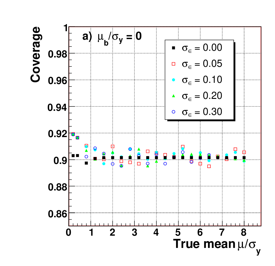
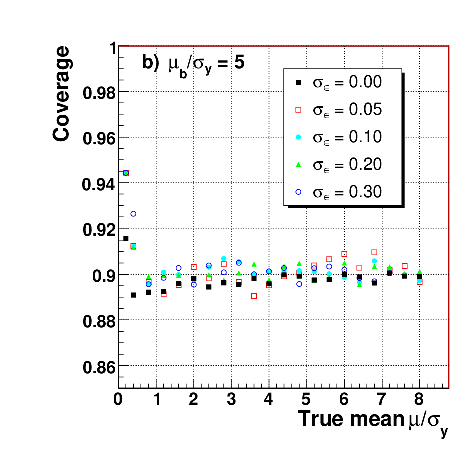
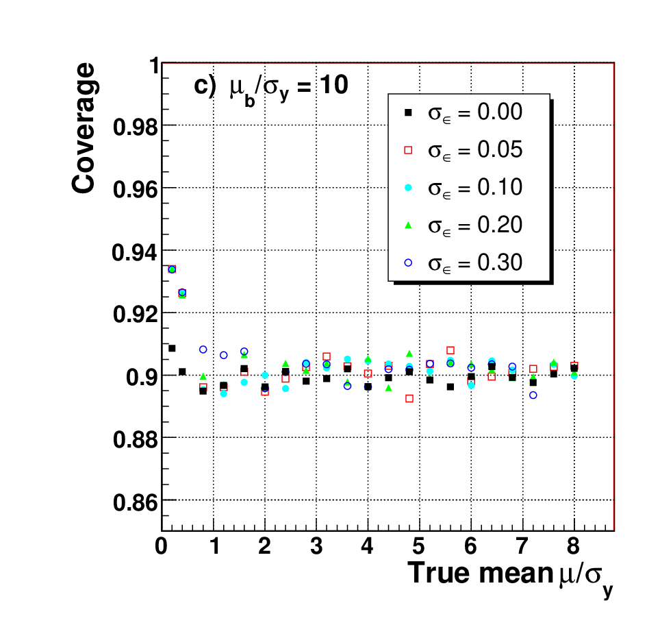
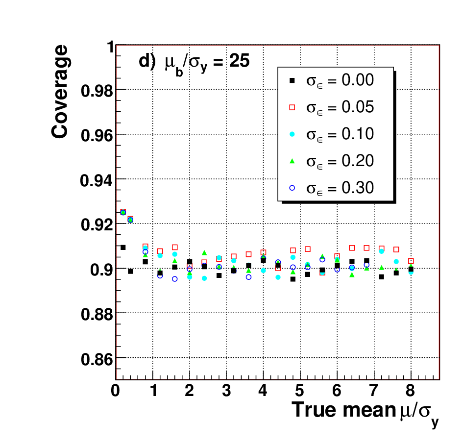
At the end of a specified number of trials (one million), the coverage was calculated as the fraction of times the true value was contained within the confidence interval. The results are shown in Fig. 4 at four values of the reduced background level for various values of . The coverage for the case of =0 was determined by generating the variable directly to avoid calculations where was very small. The figure shows that correct coverage is achieved within 1% for . For less than 0.5, there is a systematic increase of the coverage that depends on the background level. The increase is due, in part, to numerical approximations for large negative values of the measured quantity , because for small , the procedure itself should converge to the standard Feldman and Cousins result, which ignores systematic uncertainties and shows correct coverage. Punzi [13] has studied the coverage for various ordering algorithms and has shown that an ordering algorithm approximately based on the profile likelihoods can generate correct coverage for large values of the signal parameter practically independent of the scale uncertainty. However, for small values of the signal, which is governed by Poisson statistics, the coverage of this method approaches unity.
6 Example
By way of example, we take a histogram where each bin contains an estimate for the number of events above background as a function of a variable that represents, for example, the kinematic coverage of the experiment. The number of signal events is negative when the estimated background exceeds the number of measured events, and the errors on each point include the statistical uncertainties of the unsubtracted data as well as the uncertainty in the estimate of the mean background level (recall Eq. 3). The same data with its errors is shown in Fig. 5, together with lower and upper limits determined with our method for four different assumptions for the relative systematic uncertainty (=0.03, 0.10, 0.20 and 0.30). The plots provide a picture of how the systematic uncertainties might change the limits that can be set using a given data set. The limits on the first plot are very close to what would be obtained with the standard Feldman and Cousins analysis. As the systematic error increases, so do the upper limits.
7 Dependence of limits on the scale uncertainties
The application of our procedure for determining upper limits that we have described so far is quite cumbersome. Many steps of computation are required to calculate the confidence intervals, and even once determined, the limits are only valid for a fixed value of the relative scale uncertainty. If limits are to be determined for a fixed value of , as in the previous example, the procedure is straightforward. However, it would not be unusual if depends, for example, on the kinematics of the experiment, which would add considerable complexity to the entire procedure. Therefore, to streamline the calculations, we have investigated, and found, a simple dependence of the limits on systematic uncertainties.
The dependence of upper limits on the scale uncertainty is of interest in its own right and was investigated in the original study by Cousins and Highland in Ref. [7]. In that low-counting application, they concluded that the upper limit with a systematic uncertainty can be calculated from the limit with no systematic error using the following formula:
| (9) |
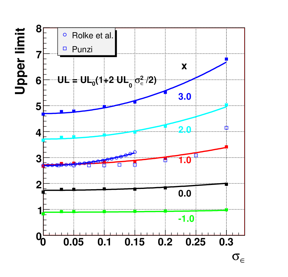
with =1. Motivated by this study, we have fitted our results to Eq. 9. For the limited range of 3, shown in Fig. 6, our results are described quite well with the empirical value of =2 if we substitute the standard Feldman and Cousins result for . We also note that this procedure has the desirable property of continuity, that is it reduces to the Feldman and Cousins result for =0. For reference, we show the dependence obtained by Rolke and collaborators in Ref. [3] and by Punzi [13] normalized to our result at , which roughly correspond to the parameters for their study. The upper limits from Rolke show a dependence consistent with a stronger dependence on the scale uncertainty with , but the data from Punzi, except for their the last point, is in very good agreement with our analysis. It must be noted, however, that these comparisons can only be qualitative, since their applications assume Poisson statistics.
In order to cover a larger range of (10), it is necessary to extend the parameterization in Eq. 9 by allowing to be a function of . Happily, the following common parameterization can be used for both upper and lower limits:
| (10) |
with = 2.26 and = 0.092 assigned for upper limits, and = 1.34 and = 0.134 used to determine the lower limits. Using this prescription, we compare our calculations for =0.3 with the scaled Feldman-Cousins result from Ref. [6] using Eq. 9. There is good agreement as shown in Fig. 7. We also note that the lower limit is relatively insensitive to the systematic error for less than 3. However, the upper limit begins deviating from the standard result for greater than 0.The deviations of the scaling from the calculations are typically within the numerical accuracy of our calculations (0.1 ), but they can be as large as 0.4 at some extremes.
8 Summary and conclusions
We have investigated how uncertainties in the estimation of the background levels and detection efficiency affect the 90% confidence intervals in the unified approach of Feldman and Cousins from Ref. [6]. The study has been conducted for experiments where the number of detected events is large and can be described by a Gaussian probability density function. The construction of confidence intervals is classical or frequentist, but the systematic uncertainties are incorporated into the construction by weighting the probability distribution with an assumed density for the nuisance parameter and then integrating over the nuisance parameter. This integration adds a Bayesian flavor to the approach as it incorporates information about our belief about the detection efficiency and the background quantities. We assume the nuisance parameters have Gaussian probability densities, and have studied the effect of relative scale uncertainties in the range between 0 0.3.
We find that the 90% confidence intervals increase quadratically with the size of the relative scale uncertainties (Eq. 9), as anticipated from previous work. The confidence intervals that incorporate scale uncertainties can be obtained from the unified confidence intervals proposed by Feldman and Cousins in Ref. [6] with a simple scaling algorithm. The new intervals have several attractive features. For small values of the true mean , the scale uncertainties do not affect the confidence intervals, as one might expect. By construction, the confidence intervals should have correct coverage, and this has been verified by Monte Carlo calculations. Finally, in the limit that approaches 0, the intervals reproduce the intervals by Feldman and Cousins that ignore systematic uncertainties.
9 Acknowledgments
This work was supported by the U.S. Department of Energy contract DE-AC05-06OR23177, under which Jefferson Science Associates, LLC operates the Thomas Jefferson National Accelerator Facility. We would like to thank Hovanes Egiyan for useful discussion and valuable suggestions, and to Kandice Carter for helpful suggestions to improve the manuscript.
References
- [1] Joel Heinrich and L. Lyons. Systematic errors. Ann. Rev. Nucl. Part. Sci., 57:145–169, 2007.
- [2] R. D. Cousins. Treatment of nuisance parameters in high energy physics, and possible justifications and improvements in the statistics literature. Prepared for PHYSTATO5: Statistical Problems in Particle Physics, Astrophysics and Cosmology, Oxford, England, United Kingdom, 12-15 Sep 2005.
- [3] Wolfgang A. Rolke, Angel M. Lopez, and Jan Conrad. Confidence Intervals with Frequentist Treatment of Statistical and Systematic Uncertainties. Nucl. Instrum. Meth., A551:493–503, 2005.
- [4] Jan Conrad, O. Botner, A. Hallgren, and Carlos Perez de los Heros. Including systematic uncertainties in confidence interval construction for Poisson statistics. Phys. Rev., D67:012002, 2003.
- [5] Fredrik Tegenfeldt and Jan Conrad. On Bayesian treatment of systematic uncertainties in confidence interval calculations. Nucl. Instrum. Meth., A539:407–413, 2005.
- [6] Gary J. Feldman and Robert D. Cousins. A Unified approach to the classical statistical analysis of small signals. Phys. Rev., D57:3873–3889, 1998.
- [7] Robert D. Cousins and Virgil L. Highland. Incorporating systematic uncertainties into an upper limit. Nucl. Instrum. Meth., A320:331–335, 1992.
- [8] M.R. Convery. Incorporating multiplicative systematic errors in branching ratio limits. SLAC-TN-03-001, February 2003.
- [9] K. Stenson. A more exact solution for incorporating multiplicative systematic uncertainties in branching ratio limits. [arXiv:physics/0605236], May 2006.
- [10] E.S. Smith. Feldman-cousins method for gaussian statistics. CLAS-NOTE 2007-019, September 2007.
- [11] E.S. Smith. Multiplicative scale uncertainties in the unified approach of feldman and cousins for constructing confidence intervals. CLAS-NOTE 2008-020, September 2008.
- [12] Joel Heinrich et al. Interval estimation in the presence of nuisance parameters. 1. Bayesian approach. [arXiv:physics/0409129], 2004.
- [13] Giovanni Punzi. Ordering algorithms and confidence intervals in the presence of nuisance parameters. [arXiv:physics/0511202], 2005.