Temperature versus acceleration: the Unruh effect for holographic models
Abstract:
We analyse the effect of velocity and acceleration on the temperature felt by particles and strings in backgrounds relevant in holographic models. First, we compare accelerated strings and strings at finite temperature. We find that for fixed Unruh temperature felt by the string endpoints, the screening length is smaller for the accelerated Wilson loop than for the static one in a thermal background of the same temperature; hence acceleration provides a “more efficient” mechanism for melting of mesons. Secondly, we show that the velocity-dependence of the screening length of the colour force, previously obtained from a moving Wilson loop in a finite temperature background, is not specific for the string, but is a consequence of the generic fact that an observer which moves with constant velocity in a black hole background measures a velocity-dependent temperature. Finally, we analyse accelerated particles and strings in the AdS black hole background, and show that these feel a temperature which increases as a function of time. As a byproduct of our analysis we find a global Minkowski embedding for the planar AdS black hole.
Keywords:
AdS/CFT, phase transitions, Unruh effect1 Introduction and summary
Evidence is mounting that there are various interesting phenomena related to the behaviour of mesonic resonances at finite temperature, just above the QCD deconfinement transition. Lattice studies (see e.g. [1]) have shown that heavy quark bound states can survive rather deep into the deconfined phase, and various experimental ideas are being pursued to measure such states directly and disentangle their decay channels [2]. However, when the bound states move or accelerate with respect to the surrounding plasma, a lattice analysis becomes impossible (at least with current techniques) and other approaches are required.
Holographic methods, based on the string/gauge theory correspondence, have proven useful to analyse such dynamical situations. The correspondence maps the behaviour of strongly coupled gauge theories at finite temperature to physics of weakly coupled strings in black brane backgrounds. The gauge theories for which a string dual is known are so far unfortunately only caricatures of QCD. However, the qualitative kinematical behaviour of quark-antiquark bound states obtained with this method shows interesting similarities with results from lattice gauge theory. In confining chiral models such as those of [3] there indeed exists a phase in which there are still quark-antiquark resonances when the gluons have already deconfined, and e.g. the behaviour of their thermal masses is similar to that obtained from the lattice [4].
The main power of holographic methods, however, is that they can provide insight into the physics of more dynamical situations, in which quarks and mesons do not sit at rest with respect to the surrounding plasma. In contrast to lattice simulations, holographic methods do not require a Wick rotation to the Euclidean regime, and deal with finite temperature directly in real time. A first result in this direction was the computation of the drag force on free quarks [5, 6]. Such a drag force is not present for colour singlet states, but they do exhibit other interesting effects. In [4, 7, 8] it was shown that the temperature at which mesons dissociate decreases with increasing velocity, i.e. with increasing transverse momentum. In more detail, it was shown that the screening length of the colour force decreases with the velocity of the quark-antiquark bound state as , where is the temperature. This result has turned out to be rather robust against changes of the string/gauge theory dual, and a similar relation also holds for low-spin mesons [9] and baryons [10, 11]. Interpreted the other way around, it states that dissociation of a colour singlet is inevitable for sufficiently large velocity (or transverse momentum).
Given the usefulness of holographic models to study finite-temperature physics, and given the relation of temperature to acceleration through the Unruh effect [12], it is natural to ask whether results such as those described above have any analog for accelerated colour singlets. This question was analysed in [13], where it was shown that an interesting bound also exists on the acceleration of mesons at zero temperature. A simple relation between the maximal acceleration and the angular momentum of a meson was obtained, , where is the string tension. This result holds for strings in flat space, accelerating orthogonally to the angular momentum plane. At a technical level the computation is closely related to the computation of the angular momentum bound for holographic mesons at finite temperature [4].
As the computation of [13] was done only in flat space, the next step is obviously to combine finite-temperature backgrounds with accelerated probes. This is the topic of the present paper. We will analyse a variety of strings and particles that move with a constant velocity or acceleration in empty AdS space or in a finite-temperature holographic background. One would naively expect that an accelerated particle or string in a finite-temperature holographic background is subject to an effective temperature that is a “superposition” of the background temperature and the Hawking temperature due to the acceleration. The situation, however, turns out to be more subtle. For instance, while in flat space all particles that move with constant velocity feel the same (vanishing) temperature, this is no longer the case at non-zero temperature, as we will show below. The situation becomes even more subtle when acceleration effects are combined with a finite-temperature background.
In most physical situations, accelerations are such that the Unruh temperature is negligible. On the other hand, it is natural to expect that strong interactions produce the largest possible accelerations. An example is jet quenching inside a quark-gluon plasma, which shows that highly energetic partons are stopped in just a few fermi. It would be of great interest to understand if the large Unruh temperature that such partons would experience could have any phenomenological consequence. For a proposal in which Unruh temperature plays a relevant role for hadronic physics in a different situation, see e.g. [14].
The outcome of our analysis is interesting in a number of ways. In the first part of this paper, we analyse various moving and accelerated probes in an AdS background, which are generalisations of the configurations studied in [13]. As expected, the qualitative results of [13] persist. However, when comparing the accelerated string configurations at zero temperature with finite temperature static string configurations, we observe that acceleration is in general a more efficient method to dissociate colour singlets than temperature (in a way which will be made precise later).
Perhaps the most striking result is obtained in the second part of the paper, where we turn to finite-temperature situations. This requires us to analyse how the Hawking temperature changes when it is observed by a moving or accelerated observer.11 1 How temperature behaves under Lorentz boosts is an issue that has led to a lot of controversy in the last century; we will comment on this further in §3. It turns out that even without knowing the full evolution of an accelerated string, one can already draw strong conclusions simply based on the effective temperature felt by its centre of mass. In fact, we will show that even the velocity dependence of the screening length, is a simple consequence of the observer dependence of temperature. For accelerated motion, we will argue that the temperature rises monotonically as a function of time.
2 Temperature effects due to acceleration in curved space
In the first part of this paper we will consider temperature effects that are caused by acceleration with respect to an inertial observer in curved backgrounds. The fact that our background possesses Lorentz symmetry in the directions parallel to the boundary guarantees that any two observers which move with constant 4-velocity in directions parallel to the boundary will not accelerate with respect to each other, and will hence measure the same temperature. We will see later that this ceases to be the case when a black hole is put in the background.
In general, an arbitrarily moving observer will not be in a (local) thermal bath, and whether it is possible to define a temperature for such an observer, and which value of the temperature it measures, crucially depends on the space-time path of the observer. There are different ways in which one may try to determine the temperature which is felt by the observer. One way is to model quantum-mechanically the detector carried by the observer, and use quantum field theory to determine the spectrum which it measures (see e.g. [15]). However, this method requires at least access to the Wightman function for a scalar field on the curved background. For most backgrounds we consider in this paper, the Wightman function is not available in closed form. We will therefore employ more geometrical approaches to the problem: the surface gravity method and Global Embedding in Minkowskian Space-time method (the GEMS), which obtains an effective temperature for a path in a curved background by embedding the path in a higher-dimensional flat space. Both techniques have been used to find the temperature observed by various types of observers in a variety of backgrounds, including (A)dS, Schwarzschild and Reissner-Nordstrom [16]. Before applying these techniques, we will first revise some of the basic ideas behind them.
2.1 The surface gravity and GEMS computation of temperature
A long time ago it was shown by Unruh [12] that an observer which moves on a straight line with constant acceleration in flat space-time sees a vacuum filled with a thermal distribution of particles, and measures a temperature which is proportional to its acceleration
| (1) |
This however is not the case for a generic path in flat or curved space, on which a detector will typically not detect a thermal spectrum [17]. However, for those special orbits for which a temperature can be defined, there are two simple geometrical approaches which can be used to determine the temperature. These are the method of surface gravity and the method which uses global embedding in a (higher-dimensional) Minkowskian space-time (the GEMS method). It turns out that there are also situations when one of the methods can be used but not the other, and we will discuss such cases in §3.2.
The surface gravity approach claims that an observer following an orbit of a time-like Killing vector field measures a temperature given by Tolman’s law,
| (2) |
where denotes the Killing vector and is the surface gravity of the horizon. The surface gravity in turn is defined by
| (3) |
In this formula the horizon can be observer-dependent (e.g. it is the Rindler horizon for an accelerated particle in flat space).22 2 We note that there is freedom in the normalisation of at infinity; generically one is allowed to multiply with a constant, which preserves the property that it is a Killing vector. However, it is clear from (2) that such a freedom does not affect the measured temperature as obtained from Tolman’s law.
The alternative GEMS approach builds on the fact that any curved Lorentzian space can be embedded in some higher-dimensional flat Minkowski space, and that hence any motion in an arbitrary curved space can be equivalently described by considering motion of the particle in that higher-dimensional flat Minkowski space. If it turns out that the higher-dimensional orbit is a time-like orbit of constant higher-dimensional acceleration, then the standard Unruh arguments can be used to define the temperature. In these cases the higher-dimensional Unruh temperature takes the form of Tolman’s law, and agrees with the surface gravity computation (2). If however, the GEMS orbit turns out to be “far away” from a constant acceleration orbit, the GEMS approach cannot be used. This can happen even when the temperature in the original system shows no pathologies, so one has to be careful.
A quantitative measure of how close the local Unruh temperature is to the temperature obtained from Tolman’s law, i.e. how slow the rate of “change” of the temperature is, was proposed in [18]. This involves generalising the notion of “jerk”, being the rate of change of acceleration in classical non-relativistic mechanics. A relativistic jerk was defined as
| (4) |
where the indices and refer to the embedding in the higher-dimensional space. The GEMS approach is then valid if the dimensionless parameter ,
| (5) |
is much smaller than one. If this condition is not satisfied, the GEMS approach cannot provide information about the temperature.
2.2 Particles in AdS
2.2.1 Static particles
To illustrate the surface gravity and GEMS approaches, let us as a simple example first consider a static particle in an empty AdS space (we will use AdS5 but generalisation to AdS in different dimensions is straightforward). Staticity here can be defined with respect to either the Poincaré or the global time. The orbits of a static particle in these two coordinates are not equivalent (since the two times are not the same).
The AdS metric in Poincaré and global coordinates, respectively, are given by (we will use the mostly minus convention for the metric signature throughout this paper):
| (6) | ||||
In global coordinates the surface gravity approach trivially gives zero for a particle at rest, i.e. following an orbit of the Killing vector field . The reason is that this particle, even though it is not inertial (has non-zero proper acceleration), does not see any horizon. We note that this is different with respect to flat space, since in this case any observer with constant acceleration sees a Rindler horizon and feels a temperature.
In Poincaré coordinates, the situation is a bit different as the particle sees a Poincaré horizon at . An explicit computation for this path yields that which, using Tolman’s law, yields zero temperature.
It was shown in [16] that the surface gravity computation for the global coordinates is in agreement with the higher-dimensional Unruh (i.e. GEMS) approach. The GEMS embeddings for the zero temperature AdS space in Poincaré and global coordinates are given in appendix A.1. The six-dimensional velocities and accelerations in the embedding space are given by
| (7) | ||||
for a particle situated at the position , in Poincaré coordinates. Similarly,
| (8) | ||||
for a particle situated at the position , in global coordinates. While the norm of the acceleration vector () for the static particle Poincaré AdS is zero, it is nonvanishing for the stationary particle in global coordinates and equal to . Hence, while the Unruh relation (1) correctly yields the result that the temperature of a static observer in Poincaré coordinates is zero, its naive application leads to a non-zero and imaginary (!) temperature in global coordinates. What happens is that for , the trajectory of the particle in the GEMS cannot be associated to a hyperbolic motion. The detector-based computation of [16, 19] has shown that such an observer would indeed measure zero temperature. One might think that this happens because the detector sees no event horizon, but this argument is at most heuristic, since e.g. a detector which is uniformly accelerated during a finite amount of time also does not see any event horizon, but does measure excitations. Note that because AdS is globally non-hyperbolic, the measured temperature will generically depend on the boundary conditions at infinity. We emphasise that in the context of AdS/CFT, the appropriate boundary conditions to use are the “reflective” ones (in the terminology of [20]), see e.g. [21].
2.2.2 Accelerated particles
Let us now turn to the more interesting case of accelerated particles, that is to say, particles which move in empty AdS space in Poincaré coordinates with a constant acceleration. More precisely, we will consider particles which move such that the norm of the 4-acceleration in the directions parallel to the boundary of AdS is constant. Explicitly the path of the particle is:
| (9) |
The proper 5-acceleration for this particle is given by
| (10) |
The time-like Killing vector which is associated with this trajectory is , given in Rindler coordinates on the four-dimensional slice (i.e. and , such that an observer at constant has ). The accelerated particle observers see the Rindler horizon at . Using the surface gravity computation we find . Therefore, the temperature measured by the detector is
| (11) |
This is the same result as obtained in [16] for an accelerated particle in AdS space in global coordinates.
Turning now to the GEMS computation of the temperature, we first determine the velocity and acceleration in the embedding space. The path under consideration leads to
| (12) | ||||
The modulus of the acceleration in the embedding 6-dimensional space () is:
| (13) |
From we then, consistently, recover the result (11).
2.3 Strings in AdS
Having discussed the effect of velocity and acceleration on the Unruh temperature observed by particles in AdS, let us now turn to strings. We will first consider Wilson loops, i.e. string configurations corresponding to non-dynamical (i.e. infinite mass) quark-antiquark pairs, and will then generalise these to finite-mass meson configurations. The endpoints of a Wilson loop can be accelerated either longitudinally, i.e. along the direction of separation of the endpoints (§2.3.1), or in a direction orthogonal to the separation (§2.3.3). For the latter case we compare accelerated loops at zero temperature with static loops at finite temperature. We then consider more complicated accelerated situations, namely finite quark-mass situations (§2.3.4) and rotating mesons (§2.3.5).
2.3.1 Longitudinally accelerated Wilson loops
Let us consider a Wilson loop whose endpoints are separated in the direction, and which accelerates in that same direction.33 3 In flat space, a string which extends in the direction in which it moves also experiences an acceleration bound, obtained by demanding that the endpoints do not lose causal contact. This situation is closely related to Bell’s space-ship “paradox” [22], and has been analysed in a large number of papers (see e.g. [23, 24]). The difference with our setup here is that we have an extra, holographic, direction in which the string extends. In the following, it will be convenient to define a different radial variable in the Poincare AdS metric (6), namely:
| (14) |
To describe such a string only the coordinates will play a role. The relevant part of the AdS metric is
| (15) |
To describe acceleration, it is convenient to make a change to Rindler coordinates
| (16) |
such that a particle at constant is uniformly accelerated, with 4-acceleration . The metric is then
| (17) |
This metric has two horizons: the Poincaré horizon at and the Rindler horizon at . We want to consider a string which is static with respect to the -time. The accelerations of all points on the string worldsheet are thus constant (but not equal to each other).


Going to the static gauge , , , we write the Nambu-Goto action as:
| (18) |
The equation of motion takes the form,
| (19) |
We want to solve this equation by imposing the boundary conditions that the string endpoints are located at the boundary and move with accelerations and .
Expanding equation (19) around one gets a two-parameter family of solutions describing the motion of each end of the string,
| (20) |
where and are integration constants. Regularity of the solution uniquely fixes and in terms of the parameters on left-hand side, which means that (as expected) the second order equation has two independent parameters. In fact, because of the underlying rescaling symmetry, and are just functions of .
Hence the nature of the solution only depends on the value of the parameter . When solving the differential equation for , one finds that the other string endpoint reaches at a value of . Conversely, if , then ( and always have opposite sign). Some examples are depicted in figure 1.44 4 The static gauge described above cannot be used to obtain the complete string shapes, as the solution is multi-valued. In practise, one thus has to change between the and gauges while solving the differential equations numerically. By taking different values of we can probe all the possible values of the ratio between the acceleration of both endpoints.
Curiously, there is a minimal (and, thus, a maximal) value of this ratio, i.e. a maximal separation between the string endpoints, see figure 2. This maximal value is the analogue of the screening length for orthogonally accelerated Wilson loops to be discussed in §2.3.3. Following the analogy with §2.3.3, or with the well-known finite temperature case [25, 26], we expect that, to the right of the minimum of the graph (and to the left of the maximum), solutions should be perturbatively stable. Between the two local extrema, the string solutions should be unstable.55 5 Perturbative stability of string configurations associated to Wilson loops was studied in [27]; see also [28]. There should also exist a point where the string becomes metastable towards decay into two separate strings. We will not, however, pursue these issues further.

2.3.2 Accelerated single quark solution
By looking at figure 1 we see that as approaches 0, the endpoint accelerations approach each other, , and the acceleration of the midpoint of the string increases. As the separation goes to zero (), the acceleration of the midpoint becomes infinite and we are effectively left with a single trailing string, which asymptotically touches the Rindler horizon. In other words, when the Wilson loop “melts”, and dissociates into two (overlapping) isolated quarks. In this case it is actually possible to find a simple explicit solution of (19):
| (21) |
where is an integration constant which is identified with the acceleration of the isolated quark, because of the condition . One end of the string is attached to the AdS boundary and the other one sits at the Rindler horizon. The profile (21) is, when compared to the finite temperature case of [25, 26], the analogue of a straight string hanging from the boundary to the AdS black hole horizon.66 6 After completion of this work we were informed that this solution has previously been found in a different context [29], and was further analysed in [30], where the connection to the Unruh effect was pointed out (see [31] for a numerical analysis of generalisations of this solution to finite temperature). However, the global properties of their solution are different and lead to a horizon on the worldsheet. Our analysis gives an alternative interpretation of the exact solution as a limit of the numerical solutions discussed in the previous section.
2.3.3 Orthogonally accelerated Wilson loops: temperature vs. acceleration
For particles, we know that temperature and linear acceleration are interchangeable, by virtue of the Unruh effect. The situation is more subtle for strings as different points on a string in general have different acceleration. However, ignoring for the moment the details of the string profiles, one may try to compare various physical quantities, like for example screening lengths, in situations where they are caused either by thermal effects or by acceleration. In the present section we will compute the possible profiles of a Wilson loop accelerated in the direction, orthogonal to the quark separation along , and compare it to the results for a static Wilson loop in a finite-temperature background [25, 26].
We write the relevant part of the metric as
| (23) |
We look for a solution static in . Using the gauge (so primes denote derivatives with respect to ), the Nambu-Goto action reads:
| (24) |
(We have also performed our numerical analysis using the Polyakov form, along the lines of [5], which has the disadvantage of an explicit constraint but the advantage that one can easily enforce the world-sheet coordinates to be regular). Considering a string symmetric with respect to its turning point (which we choose to be at ) such that , the equations of motion read:
| (25) |
Here the last equation in (25) is a consequence of the existence of a conserved quantity, due to the fact that the Lagrangian does not explicitly depend on . The two integration constants and correspond to the position of the midpoint of the string:
| (26) |
Equivalently these can be traded for and , the string length77 7 Here and in the following, the term string length should be understood as the separation between the endpoints in the direction transverse to acceleration. and the acceleration of the string endpoints:
| (27) |
It is interesting to see how equations (25) behave near the AdS boundary . At that point, reaches a finite value. By expanding the above equations we find (we just focus on the endpoint, expansions around are trivially obtained from the ones below due to the symmetry ):
| (28) |
Given any pair we can numerically integrate the above equations and determine . Figure 3 depicts an example.


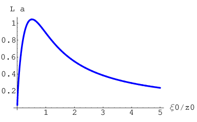
Due to the underlying conformal symmetry, a simultaneous rescaling and will just rescale the whole solution, yielding . Thus, for fixed there is a fixed value of . See figure 4. From this graph we conclude that, for a fixed acceleration, the maximum quark-antiquark separation for which a connected string solution of the Nambu-Goto action exists is:
| (29) |
In the language of the dual gauge theory, the colour force is screened for larger separation. We can also define a critical length at which the accelerated connected string becomes energetically disfavoured and, thus, metastable, with respect to two separate accelerated strings, see § 2.3.2. Even if the energy integrals are divergent, we can define a renormalised energy as the energy of the connected string minus twice the energy of a single quark string,
| (30) |
where we have inserted (22). Using the expansions (28) one can check that the divergences around cancel out. The critical length is defined as the one for which . A numerical computation produces the following approximate results:
| (31) |
We now proceed to compare these results to the case of static strings in the AdS black hole [25, 26]. For this purpose, it is useful to notice that, using (11), the ratio can be related to the Unruh temperature felt by the midpoint of the string, namely:
| (32) |
Note that this temperature has a clear-cut meaning on the string theory side, but does not necessarily translate in a straightforward way to the gauge theory side, in contrast to the endpoint temperature. We also want to compare our result to the case of a string accelerated in flat space [32, 33]. We remind the reader of the relation, in that case, between the string length, the acceleration of the string endpoints (which we denote by ) and the string midpoint acceleration,
| (33) |
from which one finds the maximal length for fixed acceleration .
The comparison between the finite acceleration and finite temperature cases is summarised in figure 5 and table 1, where we have also included the flat space result. We see that acceleration dissociates extended objects more efficiently than its associated Unruh temperature.
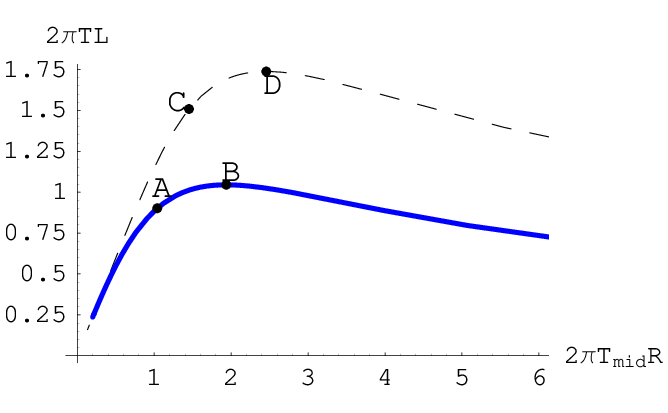
| accelerated string in AdS | 1.045 | 0.90 |
| static string in AdS black hole | 1.738 | 1.508 |
| accelerated string in flat space | 1.325 | 1.055 |
Notice that for this comparison, we need to relate the temperature of the heat bath in the formula (1) with some kind of effective temperature felt by the accelerated string. This is in principle tricky, as the string is an extended object, and different points on the string have different accelerations, and in principle feel different local Unruh temperatures. For mesons it seems natural to consider the Unruh temperature of the quarks as a relevant temperature, as this is the parameter that should be easiest to control experimentally, given that quarks are charged.
2.3.4 Orthogonally accelerated mesons


We now want to consider acceleration of finite-energy string configurations, corresponding to mesonic states with finite constituent quark masses. The simplest way of obtaining information about mesons with dynamical quarks is to consider the regularised version of the Wilson loop. That is, we will solve the same equations of motion for a U-shaped string of § 2.3.3, but with endpoints fixed at some probe brane . Then, we compute the length and acceleration of the mesonic string as
| (34) |
The relation we are after is the behaviour of the maximal acceleration of these endpoints as a function of their fixed separation . We will assume that appropriate forces have been introduced to keep this separation constant at all times, and we will thus discard any boundary terms in the equations of motion. This situation is as close as one can get to the acceleration bound found in [13] when one considers non-rotating configurations (which have their size stabilised dynamically).

To find the relation , we have determined the endpoint acceleration for various separations as a function of the midpoint acceleration. The result is displayed in figure 6 (where we have chosen the D7-brane to be located at for convenience). The points in these figures were obtained by finding such that the endpoint separation is equal to the fixed value of given in each plot, and then registering the corresponding .
By analysing the position of the maximum in as a function of , one then finds figure 7. This result is to be compared to the analysis of [32, 33], see (33). Our results for the AdS setup are qualitatively similar to this flat space result.
Alternatively, one can consider a similar U-shaped string configuration where the separation between the endpoints is determined dynamically, and stabilised by rotation of the string. To this technically more involved configuration we turn now.
2.3.5 Rotating accelerated mesons
Real world mesons have a non-vanishing angular momentum, and hence it is also interesting to analyse the behaviour of rotating string configurations in AdS. The relevant piece of the metric is
| (35) |
For the rotating string, the natural ansatz is, in terms of the worldsheet coordinates ,
| (36) |
Notice that we have already fixed part of the worldsheet reparametrisation invariance. This ansatz immediately solves the equations and constraints for and . We are left with a reduced Nambu-Goto action,
| (37) |
where a prime denotes a derivative with respect to . The equations of motion can be readily obtained from this action. An important quantity is the angular momentum,
| (38) |
Note that all these expression reduce to those of [13] if we would insert and identify , although this is of course not consistent in the present setting.
As in § 2.3.4, we will consider strings hanging from a brane at . Any solution of the reduced action (37) also solves the full Nambu-Goto action. However, not all solutions are physically consistent since the open string action has to be supplemented with a boundary condition. This was first discussed for a similar set-up in [34] where it was shown that the string had to hit the brane orthogonally. The argument is similar in the present case and leads to:
| (39) |
which, in turn, implies . Thus, for fixed , the family of solutions is therefore defined by three parameters , and . These three parameters are subject to one constraint (39), so we are left with a two-parameter family. The two parameters can be identified with the physical quantities and .


We have numerically analysed families of configurations with different values of the midpoint and endpoint acceleration. These curves exhibit a maximum in , see figure 8a. For any given there is thus a maximal , and the relation is plotted in figure 8b. Our main result is that there is an upper bound on the acceleration (beyond which no mesons exist) which scales with the angular momentum as
| (40) |
where is a positive number. This exponent equals in flat space and grows to about in the AdS background which we considered here, at least in the region of displayed in figure 8.
This concludes our analysis of accelerated strings in the zero-temperature AdS background. We will now turn to the analysis of strings in the finite-temperature AdS black hole background.
3 Velocity and acceleration effects in finite temperature backgrounds
Having discussed the Unruh effect for various observers in curved space with vanishing Hawking temperature, we now want to consider cases in which the background has a non-zero temperature. The problem of an observer moving with constant velocity through a heat bath has received considerable attention in the literature (in part because it is relevant for the interpretation of measurements of the cosmic microwave background), and we will here add some more ingredients to this debate. Briefly, such an observer sees an angle-dependent spectrum, which is thermal for each fixed angle, but with a temperature which depends on the angle between the direction of motion and the direction of observation [35, 36, 37], see also [38],
| (41) |
As explained in [39, 40], there are thus various ways to define an “effective” temperature (keeping in mind, of course, that the spectrum really is not thermal to begin with). The resulting power of will depend on the details of this averaging procedure [39]. We will see in the present section that the effective temperature observed by a moving string, in the sense of the temperature relevant for its dissociation, is in fact obtained simply from a surface gravity computation.
3.1 Constant velocity particles in the AdS-BH background
As we have emphasised in the introduction, the temperature measured by observers in finite temperature backgrounds depends in a more complicated way on acceleration and velocity than in zero temperature backgrounds. We will be interested in the case of particles and strings moving parallel to a planar AdS black hole horizon.
The simplest case one can analyse is one in which a particle-like observer moves with constant velocity at fixed distance away from a flat black hole in AdS (or in other words, on a D-brane suspended at fixed distance from the horizon). The relevant metric is
| (42) |
with , where is related to the temperature of the dual field theory as . We will consider the orbit for which . The relation between coordinate time and proper time is a function of ,
| (43) |
The velocity is thus necessarily bounded by the local velocity of light, . The Killing vector relevant for the computation of the surface gravity is
| (44) |
Evaluating the surface gravity expression (3) at the particle horizon we find
| (45) |
For the observed temperature we use the Tolman law, which in this case yields88 8 The same temperature can be obtained from a different perspective, namely by considering coordinates in which the particle is static but feels a hot wind from the plasma moving at velocity . In order to check this, one can first boost the metric (42) in the direction by changing , , which gives Computing (3) for this metric with , one finds . Upon insertion in (2) this yields (46), as expected.:
| (46) |
We should note several features of this formula. Firstly, we see that in the limit we recover the known result [19, 41] that a static observer at asymptotic infinity of the AdS-Schwarzschild black hole measures a vanishing temperature. This is in contrast with an asymptotic static observer in a flat space black hole spacetime, which measures a non-vanishing Hawking temperature.
Secondly, the behaviour of this temperature for large distance away from the horizon is remarkable. In the limit it scales with the velocity as
| (47) |
where is the local temperature for a static observer at position . This result is to be compared with the behaviour of the screening length of the colour force, found in the string computations of [4, 7, 8], and approximately given by:
| (48) |
If we use (47) at the centre-of-mass position of the string, we have and the relation (48) simply states that the screening length is inversely proportional to the observed temperature, . In [42], this result was generalised to other backgrounds different from , the main difference being the exponent of the factor. We have checked in a variety of cases that the method presented in this section reproduces the results of [42]. We want to emphasize that computations of this section do not involve any stringy action.99 9 The relevance of the temperature scale has of course been pointed out many times before (see in this context also [29] where the connection to transverse momentum broadening is discussed). Our computation shows why this scale appears naturally.
We can also try to compute the observed temperature by using an embedding in a globally Lorentzian space-time. In order to construct this embedding we need to suitably modify the embedding of the spherical AdS black hole given in [41], see appendix A.2. In this constant velocity case, however, the jerk of the associated trajectory is not small and there is no immediate interpretation from the GEMS. This corresponds to the fact, already alluded to at the beginning of this section, that the observed spectrum is only approximately thermal. It could prove interesting to tackle this problems with methods similar to [43], but we will not attempt that here.
3.2 Accelerated particles in the planar AdS black hole
For an accelerated string in an AdS black hole background, the equations of motion are much more complicated than for the constant velocity case discussed in the previous subsection. We will comment on these string configurations in the next subsection. Before we do so, let us first again try to get an intuition for the physics by analysing the much simpler case of a point particle.
The point particle we will analyse here is one which is accelerating parallel to the flat horizon of a planar AdS black hole. We want to consider a particle with a constant 4-acceleration. This is similar to the computation of §2.2.2, but now for the black hole case. The particle follows the path
| (49) |
Note that in order to ensure that the particle has a constant 4-acceleration we have to include the factor , which accounts for the fact that there is a non-trivial red-shift between two different values of the radial coordinate.
We will attempt to compute the temperature observed by this particle using the GEMS approach. By using the GEMS embedding of the planar AdS black hole (56) we compute the norm of the higher-dimensional GEMS acceleration,
| (50) |
We see that, unlike in all previous cases, this norm has a polynomial dependence on time. The jerk modulus is non-zero and also grows in time,
| (51) |
We can now compute the parameter (5) which measures the applicability of the GEMS approach,
| (52) |
We see that is independent of the radial position of the particle, but depends on time. Actually, we see that for , i.e. it is not possible to choose parameters in such a way that remains small for all times.
Nevertheless, notice that the jerk modulus and, accordingly, , vanish at (actually the whole jerk vector vanishes at this point, not just its modulus). Thus, we can consistently define an effective temperature that an accelerated detector would observe at , the instant at which the velocity vanishes although the acceleration is finite1010 10 This is completely analogous to the discussion in [41], where a temperature for a freely falling observer in a black hole background could only be defined at the instant when the observer is at rest. The notion of instantaneous temperature is not well-defined and, in order for (53) to coincide with a temperature measured by our hypothetical detector, the typical time of the microscopic processes involved in the detector measurements should be much smaller than the critical time at which (53) loses its validity. In general, one should think of (53) as an effective approximate expression for the amount of heating felt by the accelerated particle.. Inserting in (50) we reach the expression:
| (53) |
where we have defined as the temperature that a static observer at the same constant would observe and as the temperature coming just from the observer acceleration in the 4-d constant slice of the geometry (the Unruh temperature for the same trajectory if in the metric (42) one discards the d term).
Hence, we conclude that an accelerated particle in the background of a planar AdS black hole, at the initial stage of the acceleration, is in an approximate state of thermal equilibrium, with a local temperature that increases in time. After a critical time , the GEMS approach can no longer be used, and we cannot say what is the final destiny of such a particle. The critical time is a complicated function of and which is a solution of a particular cubic equation .
One may wonder if the surface gravity approach could be used more successfully here. Unfortunately, the problem which one faces in this case is that unlike in all previous cases, the path which the particle follows is not generated by a Killing vector field, which prevents one from using this method.
3.3 Particles versus strings
Finding even a numerical solution of a string with accelerated endpoints in the background of an AdS black hole is a non-trivial problem. The reason is that a generic string configuration with such boundary conditions will be space-time dependent, and it is a priori not clear that it is possible to find a globally well-defined time variable in which the string motion would be static. In contrast to §2.3.4, where we used Rindler like coordinates to reduce the system of partial differential equations to an ordinary differential equation, this is now no longer possible. In addition it is also not clear which one of the many possible time-dependent solutions satisfying the boundary conditions of accelerated endpoints is the most relevant one (e.g. which one has the lowest energy, and corresponds to an unexcited accelerated meson).
However, despite all above mentioned problems and subtleties, it seems reasonable to expect that the qualitative behaviour of the accelerated meson can be extracted by considering an accelerated point particle instead of string, as a first approximation. To see what is the difference of the full (string) solution versus the particle approximation, let us consider the examples of a string in flat space and the accelerated string in AdS space. We will then compare these systems with the particle approximations.


Since the string is an extended object it is clear that if the string does not move as a rigid object, different points on its worldvolume could feel a different temperature. The explicit example of such a behaviour is provided by the string in flat space [13]. Different points on the string move with different (and constant) acceleration, with the maximal acceleration (i.e. temperature) experienced by the midpoint of the string. Figure 9 shows the dependence of the midpoint temperature on the acceleration of the string endpoints. We see that for small accelerations (when the string is almost straight in Rindler space), the midpoint feels the same temperature as the rest of the string. As the acceleration is increased, the temperature of the midpoint starts to increase faster than the linear Unruh relation between temperature and endpoint acceleration (1) (i.e. what a point particle would experience). This holds true for strings in flat space as well as for strings in AdS, but the increase is more dramatic in the latter case.
4 Discussion and outlook
In this paper we have analysed the effects of velocity and acceleration on particles and strings, both in zero and finite temperature backgrounds.
For the simplest case, in a background with zero Hawking temperature, velocity has no effects. On the other hand, it is known that a particle in flat space at constant acceleration will measure the Unruh temperature [12]. The situation for strings is more complicated. The AdS/CFT correspondence provides a perfect laboratory in which one can study the effect of acceleration for a hadronic string, as was shown in § 2.3. We found, as expected, that effects of acceleration are qualitatively similar to those of temperature. Generalising the previous analysis in flat space [32, 13], we found that there exist maximum accelerations for a string of given length or angular momentum. A surprise encountered in our analysis is that acceleration is “more efficient” than temperature in melting strings. This statement means that, for a string of a given length, the Unruh temperature of the string endpoints for which the string melts is smaller than the Hawking temperature at which the static string would undergo melting. Qualitative similarities and quantitative differences between temperature and acceleration for a non-rotating string are summarised in figure 5.
When a finite temperature background is considered, we have seen that velocity and acceleration produce independent effects which raise the observed temperature. This is apparent from (47), where and (53) where . When both velocity and acceleration are present, the situation is more complicated because the observed spectrum is far from thermal. In [7], it was argued that the raise in temperature due to velocity would enhance quarkonium suppression in a quark-gluon-plasma. In view of our results, it is natural to expect that if the highly energetic quarkonium state also feels a large acceleration (or better said, deceleration) within the plasma, the suppression would be enhanced further.
We see a number of directions for future study. One concerns the analysis of the effect of rotation on observed temperature. While we have so far analysed the behaviour of linearly accelerated strings, full-fledged holographic mesons also contain an acceleration component due to the orbital motion. It is known that orbital motion itself does not lead to the observation of a thermal bath. However, the spectrum of vacuum fluctuations is to good approximation thermal, and determines the response of a detector [17]. For the superposed motion of angular and linear acceleration, the Unruh effect has been studied in flat space-time by [44, 45]. Generically, for fixed linear acceleration, the effective temperature of the vacuum fluctuations is higher when there is a non-zero angular component. It would be interesting to understand such computations in a holographic context.
On a more fundamental level, it would be interesting to develop a better understanding of the velocity dependence of temperature in the context of general relativity. We have seen that the surface gravity and GEMS methods both lead to a velocity dependence of the temperature which is similar to the average of the angle-dependent temperature obtained using other techniques. A proper understanding of this is lacking, and requires a more detailed quantum-field theoretical analysis, which might be feasible in a lower dimensional toy model. We hope to return to these questions in future work.
Acknowledgements
AP thanks Kevin Goldstein for discussions. The work of AP & KP was supported in part by VIDI grant 016.069.313 from the Dutch Organisation for Scientific Research (NWO). The work of AP is also partially supported by EU-RTN network MRTN-CT-2004-005104 and INTAS contract 03-51-6346. KP thanks the University of Durham for kind hospitality.
Appendix A Appendix: technical details
A.1 GEMS for AdS in global and Poincaré coordinates
The AdS space can be seen as a hyper-cylinder embedded in a signature (2,4) Minkowski space
| (54) |
A GEMS embedding of space in Poincaré coordinates (6) into a signature (2,4) Minkowski space is given by
A GEMS embedding of the space in global coordinates is similarly given by
| (55) | ||||
A.2 GEMS for AdS-Schwarzschild black hole in Poincaré coordinates
Let us consider a (3,5)-signature Minkowski space-time with signature . We introduce
| (56) |
If we insert these expressions into
| (57) |
we recover the metric (42). It is not hard to check that the GEMS computation using the above embedding yields the correct observed temperature for a static observer (i.e. sitting at constant ) which is obtained by setting in equation (46).
References
- [1] G. Aarts, C. Allton, M. B. Oktay, M. Peardon, and J.-I. Skullerud, “Charmonium at high temperature in two-flavor QCD”, Phys. Rev. D76 (2007) 094513, arXiv:0705.2198.
- [2] PHENIX Collaboration, S. X. Oda, “ production at RHIC-PHENIX”, arXiv:0804.4446.
- [3] T. Sakai and S. Sugimoto, “Low energy hadron physics in holographic QCD”, Prog. Theor. Phys. 113 (2005) 843–882, hep-th/0412141.
- [4] K. Peeters, J. Sonnenschein, and M. Zamaklar, “Holographic melting and related properties of mesons in a quark gluon plasma”, Phys. Rev. D74 (2006) 106008, hep-th/0606195.
- [5] C. P. Herzog, A. Karch, P. Kovtun, C. Kozcaz, and L. G. Yaffe, “Energy loss of a heavy quark moving through supersymmetric Yang-Mills plasma”, JHEP 07 (2006) 013, hep-th/0605158.
- [6] S. S. Gubser, “Drag force in AdS/CFT”, Phys. Rev. D74 (2006) 126005, hep-th/0605182.
- [7] H. Liu, K. Rajagopal, and U. A. Wiedemann, “An AdS/CFT calculation of screening in a hot wind”, Phys. Rev. Lett. 98 (2007) 182301, hep-ph/0607062.
- [8] M. Chernicoff, J. A. Garcia, and A. Guijosa, “The energy of a moving quark-antiquark pair in an SYM plasma”, JHEP 09 (2006) 068, hep-th/0607089.
- [9] Q. J. Ejaz, T. Faulkner, H. Liu, K. Rajagopal, and U. A. Wiedemann, “A limiting velocity for quarkonium propagation in a strongly coupled plasma via AdS/CFT”, JHEP 04 (2008) 089, arXiv:0712.0590.
- [10] C. Athanasiou, H. Liu, and K. Rajagopal, “Velocity dependence of baryon screening in a hot strongly coupled plasma”, JHEP 05 (2008) 083, arXiv:0801.1117.
- [11] C. Krishnan, “Baryon dissociation in a strongly coupled plasma”, arXiv:0809.5143.
- [12] W. G. Unruh, “Notes on black hole evaporation”, Phys. Rev. D14 (1976) 870.
- [13] K. Peeters and M. Zamaklar, “Dissociation by acceleration”, JHEP 01 (2007) 038, arXiv:0711.3446.
- [14] P. Castorina, D. Kharzeev, and H. Satz, “Thermal hadronization and hawking-unruh radiation in qcd”, Eur. Phys. J. C52 (2007) 187–201, arXiv:0704.1426.
- [15] N. D. Birrell and P. C. W. Davies, “Quantum fields in curved space”, Cambridge University Press, 1982.
- [16] S. Deser and O. Levin, “Mapping Hawking into Unruh thermal properties”, Phys. Rev. D59 (1999) 064004, hep-th/9809159.
- [17] J. R. Letaw and J. D. Pfautsch, “The quantized scalar field in rotating coordinates”, Phys. Rev. D22 (1980) 1345.
- [18] J. G. Russo and P. K. Townsend, “Accelerating Branes and Brane Temperature”, Class. Quant. Grav. 25 (2008) 175017, arXiv:0805.3488.
- [19] S. Deser and O. Levin, “Accelerated detectors and temperature in (anti) de Sitter spaces”, Class. Quant. Grav. 14 (1997) L163–L168, gr-qc/9706018.
- [20] S. J. Avis, C. J. Isham, and D. Storey, “Quantum field theory in anti-de Sitter space-time”, Phys. Rev. D18 (1978) 3565.
- [21] A. Nunez and A. O. Starinets, “AdS/CFT correspondence, quasinormal modes, and thermal correlators in SYM”, Phys. Rev. D67 (2003) 124013, hep-th/0302026.
- [22] J. S. Bell, “Speakable and unspeakable in quantum mechanics. Collected papers on quantum philosophy”, Cambridge University Press, 1987.
- [23] M. Gasperini, “Causal horizons, accelerations and strings”, Gen. Rel. Grav. 24 (1992) 219–223.
- [24] M. McGuigan, “Finite black hole entropy and string theory”, Phys. Rev. D50 (1994) 5225–5231, hep-th/9406201.
- [25] S.-J. Rey, S. Theisen, and J.-T. Yee, “Wilson-Polyakov loop at finite temperature in large- gauge theory and anti-de Sitter supergravity”, Nucl. Phys. B527 (1998) 171–186, hep-th/9803135.
- [26] A. Brandhuber, N. Itzhaki, J. Sonnenschein, and S. Yankielowicz, “Wilson loops in the large- limit at finite temperature”, Phys. Lett. B434 (1998) 36–40, hep-th/9803137.
- [27] S. D. Avramis, K. Sfetsos, and K. Siampos, “Stability of strings dual to flux tubes between static quarks in SYM”, Nucl. Phys. B769 (2007) 44–78, hep-th/0612139.
- [28] J. J. Friess, S. S. Gubser, G. Michalogiorgakis, and S. S. Pufu, “Stability of strings binding heavy-quark mesons”, JHEP 04 (2007) 079, hep-th/0609137.
- [29] F. Dominguez, C. Marquet, A. H. Mueller, B. Wu, and B.-W. Xiao, “Comparing energy loss and -broadening in perturbative QCD with strong coupling SYM theory”, Nucl. Phys. A811 (2008) 197–222, arXiv:0803.3234.
- [30] B.-W. Xiao, “On the exact solution of the accelerating string in space”, Phys. Lett. B665 (2008) 173–177, arXiv:0804.1343.
- [31] M. Chernicoff and A. Guijosa, “Acceleration, energy loss and screening in strongly-coupled gauge theories”, JHEP 06 (2008) 005, arXiv:0803.3070.
- [32] V. P. Frolov and N. G. Sanchez, “Instability of accelerated strings and the problem of limiting acceleration”, Nucl. Phys. B349 (1991) 815–838.
- [33] D. Berenstein and H.-J. Chung, “Aspects of open strings in Rindler space”, arXiv:0705.3110.
- [34] M. Kruczenski, D. Mateos, R. C. Myers, and D. J. Winters, “Meson spectroscopy in AdS/CFT with flavour”, JHEP 07 (2003) 049, hep-th/0304032.
- [35] R. N. Bracewell and E. K. Conklin, “An observer moving in the K radiation field”, Nature 219 1343.
- [36] P. J. E. Peebles and D. T. Wilkinson, “Comment on the anisotropy of the primeval fireball”, Phys. Rev. 174 (1968) 2168–2168.
- [37] G. R. Henry, R. B. Feduniak, J. E. Silver, and M. A. Peterson, “Distribution of black body cavity radiation in a moving frame of reference”, Phys. Rev. 176 (1968) 1451–1455.
- [38] R. Aldrovandi and J. Gariel, “On the riddle of the moving thermometers”, Phys. Lett. A170 (1992) 5.
- [39] S. S. Costa and G. E. A. Matsas, “Temperature and relativity”, Phys. Lett. A209 (1995) 155, gr-qc/9505045.
- [40] P. T. Landsberg and G. E. A. Matsas, “Laying the ghost of the relativistic temperature transformation”, Phys. Lett. A223 (1996) 401–403, physics/9610016.
- [41] E. J. Brynjolfsson and L. Thorlacius, “Taking the Temperature of a Black Hole”, JHEP 09 (2008) 066, arXiv:0805.1876.
- [42] E. Caceres, M. Natsuume, and T. Okamura, “Screening length in plasma winds”, JHEP 10 (2006) 011, hep-th/0607233.
- [43] H.-Z. Chen, Y. Tian, Y.-H. Gao, and X.-C. Song, “The GEMS approach to stationary motions in the spherically symmetric spacetimes”, JHEP 10 (2004) 011, gr-qc/0409107.
- [44] J. R. Letaw and J. D. Pfautsch, “The quantized scalar field in the stationary coordinate systems of flat space-time”, Phys. Rev. D24 (1981) 1491.
- [45] J. R. Letaw and J. D. Pfautsch, “The stationary coordinate systems in flat space-time”, J. Math. Phys. 23 (1982) 425.