An Entropy Inequality

Meik Hellmund Affiliation: Mathematisches Institut, Universität Leipzig, Johannisgasse 26, D-04103 Leipzig, Germany Email: Meik.Hellmund@math.uni-leipzig.de Armin Uhlmann Affiliation: Institut für Theoretische Physik, Universität Leipzig, Vor dem Hospitaltore 1, D-04103 Leipzig, Germany Email: Armin.Uhlmann@itp.uni-leipzig.de

August 24, 2026

Abstract

Let $S(\rho)=-\Tr(\rho\log\rho)$ be the von Neumann entropy of an $N$ -dimensional quantum state $\rho$ and $e_{2}(\rho)$ the second elementary symmetric polynomial of the eigenvalues of $\rho$ . We prove the inequality

S(\rho)\;\leq\;c(N)\;\sqrt{e_{2}(\rho)}\;

where $c(N)=\log(N)\,\sqrt{\frac{2N}{N-1}}$ . This generalizes an inequality given by Fuchs and Graaf [1] for the case of one qubit, i.e., $N=2$ . Equality is achieved if and only if $\rho$ is either a pure or the maximally mixed state. This inequality delivers new bounds for quantities of interest in quantum information theory, such as upper bounds for the minimum output entropy and the entanglement of formation as well as a lower bound for the Holevo channel capacity.

pacs

03.67.-a, 03.67.Mn

I Introduction

Let $\rho$ be a density matrix of a qubit with eigenvalues $x$ and $1-x$ ( $0\leq x\leq 1$ ). Its von Neumann entropy is given by

S(\rho)=\eta(x)+\eta(1-x)

(1)

where the abbreviation $\eta(x):=-x\,\log x$ with $\eta(0)=0$ is used.¹¹ 1 Our formulas are valid for arbitrary bases of the logarithm. The natural logarithm is used in the figures. In [1] Fuchs and Graaf stated the inequality

S(\rho)\leq 2(\log 2)\sqrt{x(1-x)}

(2)

which can be read off from figure 1.

Refer to caption — Figure 1: The Fuchs-Graaf inequality.

To gain the desired extension of eq. (2) to $N$ -dimensional quantum systems, we at first observe that its right hand side is 1-homogeneous in $x_{1}=x$ , $x_{2}=1-x$ . Therefore after replacing $S$ by $(\Tr\rho)S(\rho[\Tr\rho]^{-1})$ , the inequality becomes valid for all positive matrices, not only for density matrices satisfying $\Tr\rho=1$ .

Accordingly, we define for any positive hermitian $N\times N$ -matrix $\rho$ with eigenvalues $x_{i}$

	$\displaystyle S_{1}(\rho)$	$\displaystyle=$	$\displaystyle(\Tr\rho)S(\frac{\rho}{\Tr\rho})=\sum\eta(x_{i})-\eta(\sum x_{i})$		(3)
	$\displaystyle e_{2}(\rho)$	$\displaystyle=$	$\displaystyle\frac{1}{2}\left((\Tr\rho)^{2}-\Tr\rho^{2}\right)=\sum_{i<j}x_{i}x_{j}$		(4)

The homogenized entropy $S_{1}$ is of degree one, $S_{1}(\lambda\rho)=\lambda S_{1}(\rho)$ , and it clearly coincides with $S$ at density matrices. $S_{1}$ is non-negative, concave, and super-additive on the cone of positive matrices, see for instance [2]. Similarly, $\sqrt{e_{2}}$ is of degree one. It is concave and super-additive for positive matrices. The two functions eq. (3) are bounded from above according to

	$\displaystyle S(\rho)$	$\displaystyle\leq$	$\displaystyle\frac{\Tr\rho}{N}\;S(\mathbb{1})=\log(N)\,\Tr\rho$		(5)
	$\displaystyle e_{2}(\rho)$	$\displaystyle\leq$	$\displaystyle\left(\frac{\Tr\rho}{N}\right)^{2}\,e_{2}(\mathbb{1})=\frac{N-1}{2N}\,(\Tr\rho)^{2}$		(6)

The central result of our paper is as following

Theorem 1.

For all positive semi-definite $N\times N$ matrices $\rho$ we have

S_{1}(\rho)\;\leq\;c_{N}\,e^{1/2}_{2}(\rho),\qquad\text{where}\quad c_{N}=(\log N)\sqrt{\frac{2N}{N-1}}\;.

(7)

Equality is achieved if and only if either $\rho$ is of rank one (and both sides of the inequality vanish) or if $\rho$ is proportional to $\mathbb{1}$ .

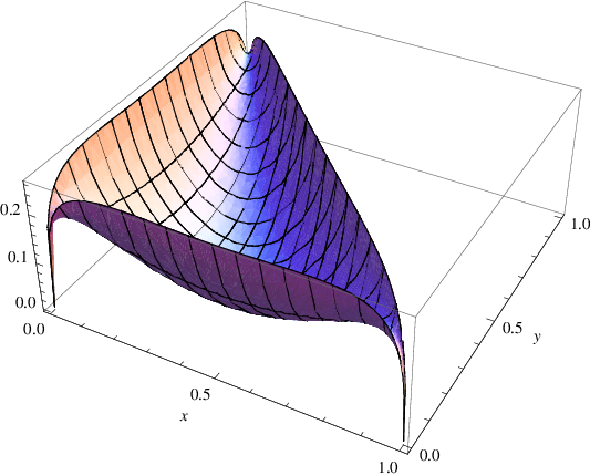
As an illustration of the theorem we show the difference between the right and the left hand side of this inequality for the case $N=3$ and $\Tr\rho=1$ . The difference vanishes at the corners (pure states) and at the center (maximally mixed state). It takes its maximum along the edges, i.e., for rank 2 states.

Before giving the proof of this theorem we add some observations.

Remark 1: $c_{N}$ is strictly increasing with $N$ .
Remark 2: If $\rho$ is of rank $k$ then the operator is supported by a $k$ -dimensional subspace. Using this sub-space, we see that eq. (7) remains valid after replacing $N$ by the rank of $\rho$ . By this argument we see that it suffices to prove eq. (7) for matrices with maximal rank.
Remark 3: Below we shall use the notation

f(\rho)=f(x_{1},\dots,x_{N})=\frac{S_{1}(\rho)}{\sqrt{e_{2}(\rho)}}

(8)

where $x_{1},\dots,x_{N}$ denote the eigenvalues of $\rho$ . We will prove that this function takes its global maximum at $\rho=\lambda{\mathbb{1}}$ . Numerical checks (up to $N=8$ ) support the more general
Conjecture: This function $f$ is concave on the set of density operators.
Remark 4: In [3], Mitchison and Jozsa considered the entropy as function of the elementary symmetric polynomials $e_{2}(\rho),\dots,e_{n}(\rho)$ defined by, e.g.,

\det(\lambda{\mathbb{1}}-\rho)=\lambda^{N}-e_{1}(\rho)\lambda^{N-1}+e_{2}(\rho)\lambda^{N-2}-\cdots+(-1)^{N}e_{N}(\rho)

(9)

They showed that $\frac{\partial S}{\partial e_{k}}>0$ for all $2\leq k\leq n$ (and therefore $\frac{\partial S_{1}}{\partial e_{k}}>0$ for all $1\leq k\leq n$ .) In the light of this it seems natural to ask for the possibility of other estimates of the entropy, for instance by using higher symmetric polynomials.

II Proof

Abbreviating $x=\sum_{m=1}^{N}x_{m}$ , $N\geq 2$ , we consider the function eq. (8),

f_{N}(x_{1},\dots,x_{N})=\frac{S_{1}(x_{1},\dots,x_{N})}{e_{2}^{1/2}(x_{1},\dots,x_{N})}=\frac{\sum\eta(x_{i})-\eta(x)}{(\sum_{i<k}x_{i}x_{k})^{1/2}}.

(10)

According to remark 2 we have to ask for extrema on $x_{m}>0$ . This implies $x>x_{m}$ for all $m=1,\dots,N$ . We use $\frac{\partial}{\partial x_{m}}e_{2}=x-x_{m},$ $\frac{\partial}{\partial x_{m}}\eta(x)=-1-\log(x),$ $\frac{\partial}{\partial x_{m}}S_{1}=\log\frac{x}{x_{m}}$ to get

\frac{\partial f_{N}}{\partial x_{m}}=e_{2}^{-1/2}\left(\log\frac{x}{x_{m}}\right)-\frac{1}{2}(x-x_{m})e_{2}^{-3/2}S_{1}.

(11)

We look for extrema of $f_{N}$ under the condition $x=const.$ They must obey

\frac{\partial f_{N}}{\partial x_{m}}=\lambda\frac{\partial x}{\partial x_{m}}=\lambda,\qquad m=1,\dots,N

(12)

Now $f_{N}$ is homogeneous of degree zero and $x$ of degree one. Therefore,

\sum_{m}x_{m}\,\frac{\partial f_{N}}{\partial x_{m}}=0,\quad\sum x_{m}\frac{\partial x}{\partial x_{m}}=x\;.

(13)

Hence, eqs. (12) can have solutions only for $\lambda=0$ . Now eq. (12) reads

e_{2}^{-1/2}(\log x-\log x_{m})=\frac{1}{2}(x-x_{m})e_{2}^{-3/2}S_{1},\qquad m=1,\dots,N

(14)

or,

\frac{\log x-\log x_{m}}{x-x_{m}}=\frac{1}{2}e_{2}^{-1}S_{1},\qquad m=1,\dots,N

(15)

Now $x>x_{m}$ for all $m$ by assumption. One knows that

x\mapsto\frac{\log y-\log x}{y-x}

(16)

is strictly decreasing for $y>x>0$ . Therefore, all $x_{m}$ must be equal and

x_{m}=\frac{x}{N},\qquad m=1,\dots,N

(17)

It is easy to check that this extremum is a maximum and therefore

f_{N}(x_{1},\dots,x_{N})\leq\frac{S_{1}(\mathbb{1})}{e_{2}^{1/2}(\mathbb{1})}=\sqrt{\frac{2N}{N-1}}\;\log N

(18)

As this maximum is increasing with $N$ , we are done.

III Applications

Let $\Phi:\rho_{in}\mapsto\rho_{out}=\Phi(\rho_{in})$ be a channel or, more general, a trace preserving positive map between two finite-dimensional quantum state spaces.

III.1 The minimum output entropy

The minimum output entropy, $S_{\rm min}(\Phi)$ , is the minimum of $S(\Phi(\rho))$ where $\rho$ is running through all density operators. Obviously, $S_{\rm min}(\Phi)$ is smaller than the minimal value of $c_{N}\sqrt{e_{2}(\Phi(\rho))}$ , where $\rho$ is any density operator. Because $\sqrt{e_{2}}$ is concave, its minimum is attained on rank one projection operators, i.e., pure states. By our theorem we get the estimate

S_{\rm min}(\Phi)\leq(\log n)\sqrt{\frac{n}{n-1}}\;\min_{|\psi\rangle}\sqrt{1-\Tr\Phi(|\psi\rangle\langle\psi|)^{2}}\;

(19)

where the minimum runs through all unit vectors $|\psi\rangle$ and $n$ is the maximal rank attained by density operators of the form $\Phi(|\psi\rangle\langle\psi|)$ .

III.2 A bound for the entanglement of formation by the concurrence

The entanglement of formation of a bipartite pure state is defined as the von Neumann entropy of one of the subsystems

E_{F}(\psi)=S\left(\Tr_{B}(\pi_{\psi})\right)\quad\text{ where }\pi_{\psi}=|\psi\rangle\langle\psi|

(20)

and extends to mixed bipartite states by the convex roof construction

E_{F}(\rho)=\min_{\sum p_{i}\pi_{i}=\rho}\;\sum\,p_{i}\,S(\Tr_{B}(\pi_{i}))

(21)

where the minimum is taken over all convex decompositions of $\rho$ into a mixture of pure states $\pi_{i}$ , see Bennett et al [4]. Another important entanglement measure is the concurrence, originally introduced for 2-qubit systems, see [5] for a review. A possible generalization to larger systems proposed by Rungta et al [6] makes again use of the second symmetric polynomial:

C(\rho)\;=\;2\min_{\sum p_{i}\pi_{i}=\rho}\;\sum\,p_{i}\,e_{2}(\Tr_{B}(\pi_{i}))^{1/2}

(22)

By theorem 1 every right hand side sum of eq. (21) can be bounded by a multiple of that of eq. (22). This simple argument provides

E_{F}(\rho)\;\leq\;(\log n)\sqrt{\frac{n}{2(n-1)}}\;\;C(\rho)

(23)

with $n=\max\,{\rm rank}[\Tr_{B}(\pi)]$ the maximal rank attained by the partially traced out pure density operators.

III.3 A bound for the Holevo quantity $\chi^{*}$

For a channel map $\Phi$ one considers the Holevo quantity

\chi^{*}_{\Phi}(\rho)=S(\Phi(\rho))-\min_{\sum p_{i}\pi_{i}=\rho}\;\sum\,p_{i}\,S(\Phi(\pi_{i}))

(24)

and the $\Phi$ -concurrence

C_{\Phi}(\rho)=2\min_{\sum p_{i}\pi_{i}=\rho}\;\sum\,p_{i}\,e_{2}(\Phi(\pi_{i}))^{1/2}

(25)

Completely similar to the reasoning above we get the inequality

\chi^{*}_{\Phi}(\rho)\;\geq\;S(\Phi(\rho))-\log(n)\,\sqrt{\frac{n}{2(n-1)}}\;\;C_{\Phi}(\rho)\;.

(26)

Here $n$ is again the maximal rank of the matrices $\Phi(\pi)$ with pure $\pi$ .

References

[1] C. A. Fuchs and J. van de Graaf, IEEE Transactions on Information Theory 45, 1216 (1999), eprint quant-ph/9712042.
[2] S. P. Boyd and L. Vandenberghe, Convex Optimization (Cambridge University Press, 2004).
[3] G. Mitchison and R. Jozsa, Physical Review A 69, 032304 (2004), eprint quant-ph/0309177.
[4] C. H. Bennett, D. P. DiVincenzo, J. A. Smolin, and W. K. Wootters, Physical Review A 54, 3824 (1996), eprint quant-ph/9604024.
[5] W. K. Wootters, Quantum Information and Computation 1, 27 (2001).
[6] P. Rungta, V. Bužek, C. M. Caves, M. Hillery, and G. J. Milburn, Phys. Rev. A 64, 042315 (2001), eprint quant-ph/0102040.