Comparison of spectral slopes of Magnetohydrodynamic and Hydrodynamic turbulence and measurements of alignment effects
Abstract
We performed a series of high-resolution (up to ) direct numerical simulations of hydro and MHD turbulence. Our simulations correspond to the ”strong” MHD turbulence regime that cannot be treated perturbatively. We found that for simulations with normal viscosity the slopes for energy spectra of MHD are similar to ones in hydro, although slightly more shallower. However, for simulations with hyper viscosity the slopes were very different, for instance, the slopes for hydro simulations showed pronounced and well-defined bottleneck effect, while the MHD slopes were relatively much less affected. We believe that this is indicative of MHD strong turbulence being less local than Kolmogorov turbulence. This calls for revision of MHD strong turbulence models that assume local “as-in-hydro case” cascading. Non-locality of MHD turbulence casts doubt on numerical determination of the slopes with currently available (–) numerical resolutions, including simulations with normal viscosity. We also measure various so-called alignment effects and discuss their influence on the turbulent cascade.
Subject headings
MHD – turbulence – ISM: kinematics and dynamicsI. Introduction
Turbulence is ubiquitous in astrophysical fluids which are characterized by high Reynolds numbers. It affects key astrophysical processes, e.g. star formation (Elmegreen & Scalo 2004, McKee & Ostriker 2007). The observational signatures of turbulence are numerous and well documented. For instance, random fluctuations on all scales, which is a sign of turbulence, has been detected by a variety of observational techniques (see Crovisier & Dickey 1983, O’Dell & Castaneda, Armstrong et al. 1994, Lazarian 2009). Turbulence is universal, because the laminar flows with high Reynolds numbers are practical impossibility. It is driven by a variety of mechanisms such as supernova explosions starbursts, stellar winds, AGN jets, etc. In Keplerian flows turbulence is generated by magnetorotational instability (Velikhov 1959, Chadrasekhar 1960, Balbus & Hawley 1991). Galactic disks are subject to the cosmic ray-induced Parker’s instability (Parker 1966).
Although, historically, hydrodynamic turbulence has been applied to astrophysics, now it is accepted that for almost all astrophysical fluid flows are coupled with magnetic fields, at least on large scales. This necessitates the use of the dynamic equations that include electric currents and magnetic fields. The simplest approach in this respect is the continuous non-relativistic one-fluid description, known as magnetohydrodynamics or MHD. This approach is broadly applicable to most of the astrophysical environments, such as Solar wind, Interstellar and Intercluster Medium, molecular clouds, stars interiors, and so on, although there are some exceptions, such as ultra-relativistic jets and shocks, where full relativistic equations should be used or small scales of Molecular Clouds, where, due to relatively low ionization rate, the two-fluid description of ions and neutrals is more appropriate.
The importance of astrophysical turbulence inspires much of theoretical and numerical work aimed at understanding its properties. We should clarify, however, that there are different types of MHD turbulence. In this paper we deal with strong MHD turbulence, which can not be treated perturbatively. The theory of weak Alfvénic turbulence, which has limited applicability to astrophysics, is discussed elsewhere (Sridhar & Goldreich 1994, Ng & Bhattacharjee 1996, Lazarian & Vishniac 1999, Galtier et al. 2000, 2002). In order to study the basic properties of MHD cascade and to be able to directly compare to previous work, we restricted ourselves to so-called balanced MHD turbulence or turbulence with zero net cross-helicity. The properties of imbalanced turbulence are studied in a companion paper Beresnyak & Lazarian (2009).
The issue of the spectral slopes of MHD turbulence has caused a substantial interest recently. A sizable number of papers attempting to measure true asymptotic spectral slope of high-Reynolds number MHD turbulence from direct numerical simulations appeared to date. For example, simulations of weakly compressible MHD turbulence performed in Haugen et al. [33], Haugen et al. [34] used finite-difference code with numerical resolution of up to with explicit viscous and resistive dissipation. The energy spectral slope for MHD was observed to be shallower than which was interpreted as the influence of the bottleneck effect. Another example is the paper of Müller & Grappin [51] who measured the spectral slopes of decaying MHD turbulence without mean field and driven MHD turbulence with strong mean field. The pseudospectral method with ordinary viscosity was ran at a numerical resolution of up to . The authors argued that the slope was close to in the mean-field case.
The motivation behind these and many other papers was to understand the nature of the turbulent cascade. The turbulent energy transfer is, in a sense, a central issue of turbulence, be it hydrodynamic or MHD. And while hydrodynamic turbulence has its “Standard Model”, the nature of MHD cascade is still debated.
An important first step in turbulence theory was made by Iroshnikov (1963) and Kraichnan (1965) who noticed that there is a local magnetic field which can not be excluded by a choice of reference frame, like the average velocity in hydrodynamics. Furthermore, they assumed that turbulence is weak, because perturbations are smaller than the mean field. This implicitly assumed local isotropic dynamics and happened to be a mistake, since the turbulent cascade preferred perpendicular direction, i.e. produced perturbations that are more and more anisotropic, this way increasing interaction and preventing turbulence from becoming weak.
The understanding of various aspects of MHD turbulence, including the role of turbulence anisotropy, compressibility, etc. resulted in a number of publications (see Dobrowolny, Mangeney, & Veltri 1980, Shebalin, Matthaeus & Montgomery 1983, Montgomery & Turner 1984, Higdon 1984). For the most part of the paper we will consider incompressible MHD turbulence, which properties are dominated by the Alfvénic perturbations. Interestingly enough, some properties of Alfvénic turbulence carry over not only to nearly incompressible low Mach number flows, but also for flows with Mach numbers larger than unity (Cho & Lazarian 2003, see also §9.3).
It has been realized that interactions of Alfvénic modes in MHD turbulence has a tendency of getting stronger as the cascades unfolds. Goldreich & Sridhar (1995, henceforth GS95) proposed a particular model of strong turbulence when the interaction strength is being controlled by two competing processes: a perpendicular cascade (a concept rigorously developed in a theory of weak Alfvénic turbulence, e.g. Galtier et al 2000), which tends to increase the interaction, and a decorrelation due to cascading which tends to increase the frequency of perturbations, and thus decrease the interaction. GS95 concluded that the interaction has to be marginally strong (“critical balance”), and therefore, the cascade has to be of strong Kolmogorov type and has a spectral slope of around . Predictions of this model, such as scale-dependent anisotropy, were subsequently observed in three-dimensional simulations (Cho & Vishniac 2000, Maron & Goldreich 2001, etc).
Recently, however, a number of models, motivated by numerical spectral slopes shallower than , appeared (Boldyrev 2005, 2006, Gogoberidze 2007). The interest to this field has been heated by the numerical discovery of so-called scale-dependent polarization alignment (Beresnyak & Lazarian 2006), which was interpreted in a subsequent publication by Mason et al (2006) in favor of Boldyrev’s (2006) modification of GS95 model.
This paper is bringing attention to serious difficulties that appear when one tries to measure true asymptotic slopes from direct three-dimensional numerical simulations which have rather moderate Reynolds numbers. By comparing spectra of hydrodynamic and MHD turbulence we found that MHD turbulence might be much more nonlocal that Kolmogorov turbulence, and, therefore, require much higher resolution to obtain spectral slope by brute force approach. The second part of this paper brings polarization alignment to more numerical scrutiny and compares the simulation results to theory. Our simulations allow to test some of the existing conjectures about properties of MHD turbulence. For instance, these results allow us to reject a conjecture in Boldyrev [14] that the alignment is limited by the magnitude of local field wandering.
In what follows in §2 we describe our approach based on comparing the properties of MHD and hydrodynamic turbulence, present our numerical setup in §3, present spectra in §4, discuss anisotropy in §5, discuss the interaction weakening and the alignment effects in §6 and §7, respectively, and provide some more hints of the non-locality of the MHD cascade in §8. In §9 we compare our numerical results with the existing theoretical predictions, as well as with the previous numerical work; we also discuss the applicability of findings obtained with incompressible simulations to the real-world compressible astrophysical turbulence. Our conclusions are summarized in §10.
II. Slope measurements
Various claims were made on the value of MHD spectral slope, most of which were motivated by either Kolmogorov slope of strong turbulence (Kolmogorov 1941, GS95), or various versions of slope (Iroshnikov 1963, Kraichnan 1965, Gogoberidze 2007, Boldyrev 2006, etc). Most numerical studies aimed to confirm either of the above. A number of critical issues were overlooked, though. Below we present a novel perspective to slopes measurements in MHD. It turns out that it is incorrect to measure slopes directly from 3D numerics due to a systematic error that comes with so-called bottleneck effect. Also, it is impossible to measure MHD slope by comparison with hydro slope, because the bottleneck effect turns out to be different in hydro and MHD. This difference, however, allows us to criticize models that rely on strong local Kolmogorov cascading, such as GS95 or Boldyrev (2006) 11 1 Local cascading models normally use a formula , where is the velocity perturbation on scale , is the cascading timescale and is a constant equal to the energy dissipation rate per unit volume..
To be precise, is not the exact predicted slope for incompressible hydrodynamics. This number comes from the Kolmogorov self-similar cascade, but soon it was realized that realistic turbulence is not exactly self-similar. To correct for this, various models of intermittency were proposed (Kolmogorov 1962, Obukhov 1962), with the most popular being She-Leveque model (1994) in which the predicted slope is around . This slope was very close to what was observed in highest-resolution DNS of Kaneda et al. [37]. In the aforementioned work it was possible to separate spectrum into inertial range and relatively more flat part that was due to a bottleneck effect. Although modifications of S-L model for MHD turbulence have been proposed, numerical studies still often compare the spectrum slope with . Similarly, when one proposes a model of turbulence with spectral slope it is often that numerical studies aim to find an exact correspondence with this slope, without regard for intermittency. We believe that this is one important stumbling block in numerical determination of slopes.
The other, probably much more important misunderstanding, is to disregard the systematic error that any numerical measurement of slopes in DNS brings with it. The bottleneck effect is a pile-up of energy before the dissipation scale due to the relative lack of energy in the dissipation range [31, see, e.g.,]. Due to relatively low resolution of currently available simulations, this systematic error is always present. To make it worse, most researchers present simulations with the highest numerical resolution only. Although the amount of numerical resources available to different groups differ substantially, most “high resolution” simulations to-date have numerical boxes between and . From the point of length of inertial interval, and the influence of bottleneck effect, the differences in linear scale of the multiple of two are tiny. Another systematic error comes from the effect of the driving scale. Often there is a dip right after the driving scale, an anti-bottleneck effect of sorts, which appears, possibly, due to the excess of energy on the driving scale. We are not aware of driven turbulence simulations that were able to get rid of this effect. We belive that disregarding these two effects and present numerical slopes as having no systematic error at all is wrong.
In this paper we compare hydrodynamic and MHD energy slopes obtained with the same code, the same driving and exactly the same linear dissipation. Since there are good theoretical predictions for asymptotic isotropic hydro turbulence, we can try to use those. If one finds that the nature of energy transfer in MHD and hydro is similar (this is suggested in GS95 model where a strong local Kolmogorov-like cascade is assumed), then we can directly compare MHD and hydro slopes and make statements on MHD slope. Unfortunately, as we show in the two subsequent sections, this is not the case. The defining feature of our simulations is the use of different types of linear dissipation, namely natural viscosity and hyper-viscosity. Although there had been some similarity in spectral slopes of MHD and hydro in normal-viscous case, the hyper-viscous cases were very different. This suggests that the nature of MHD and hydro cascades are different and one can not use slope comparison between MHD and hydro to get rid of the aforementioned systematic error.
III. Numerical setup
Incompressible MHD and Navier-Stokes equations can be written in the following simple form
| (1) |
where is a solenoidal projection and (Elsasser variables) are defined in terms of velocity and magnetic field in velocity units as and . Navier-Stokes equation is a special case of equations (1), where and, therefore, both equations are equivalent with . The RHS of this equation is a linear dissipation term which is called viscosity or diffusivity for and hyper-viscosity or hyper-diffusivity for . Here we assumed that viscosity and magnetic diffusivity is the same for velocity and magnetic field. This is almost never true for realistic astrophysical plasmas. However, as long as one wants to study the dynamics of large scale turbulence, it is acceptable. This is because the dissipation terms in today’s numerical simulations are never as small as to simulate real physical dissipation, instead, they are used to remove energy on small scales and assure stability of the code. In finite-difference codes a numerical dissipation is always present and the linear dissipation terms are often omitted altogether (see, e.g., Stone et al 1998). In pseudospectral code, such as our own, the energy is conserved with rather good precision, so the use of linear dissipation is necessary.
| Run | x:y:z | dissip. | ||||
|---|---|---|---|---|---|---|
| H1 | 1:1:1 | – | 16 | |||
| H2 | 1:1:1 | – | 10 | |||
| H3 | 1:1:1 | – | 7 | |||
| M1 | 1:1:1 | 1 | 24 | |||
| M2 | 1:1:1 | 0 | 10 | |||
| M3 | 1:1:1 | 1 | 10 | |||
| M4 | 10:1:1 | 10 | 10 | |||
| M5 | 10:1:1 | 10 | 10 |
We evolved incompressible MHD and Navier-Stokes equations in time using a well-known pseudospectral technique [22, see, e.g.,]. We have chosen pseudospectral code as it allows precise control over dissipation. Our hydro code was identical to the MHD one, except, naturally, for the lack of magnetic field. The summary of high-resolution runs is presented in Table 1.
We performed four types of simulations: a simulation of statistically isotropic hydro turbulence; a simulation of well-developed stationary MHD turbulence without mean field (), which also has been called statistically isotropic MHD turbulence; a simulation of so-called transAlfvénic turbulence (with , ); a simulation of strong anisotropic subAlfvénic turbulence (with , ). Special attention had to be taken to the last case, where, in order for the turbulence to be strong, the fields had to be strongly anisotropic on the outer scale. To ensure this, the numerical box was elongated in real space and x-direction (a direction of the strong mean field) was 10 times longer than y and z directions. The driving had anisotropy that corresponded to the dimensions of the box. Thus in this case our setup is similar to one in Maron & Goldreich [47].
We used random solenoidal velocity driving in k-space between k=2 and 3.5. The largest coherent eddy size L (determined by structure function technique) was around 1/4 of a box size () and the eddy turnover time for this scale was around unity. The Alfvénic self-crossing time for this scale was also around unity 22 2 In the strong field case, , the Alfvén speed was ten times higher, but the largest coherent eddy was elongated with x/y aspect ratio of around 10, so this gives the same estimate for Alfvénic crossing time.. The self-correlation timescale for our driving force was for all wavemodes. This is somewhat longer than the eddy turnover time. We performed a test study of the force correlation time influence on the self-correlation time of velocity, taking and found no systematic dependence. The self-correlation timescale of velocity was always around unity. We concluded that, in the case of strong turbulence, the self-correlation timescale of velocity is primarily determined by nonlinear interaction, rather than driving 33 3 One can argue that in case of the absence of nonlinear term the equation will give infinite correlation time for even if self-correlation time is finite.. We ran another, higher resolution simulation, trying to find a difference in slopes between simulations with and and found none. Note, that numerical studies do vary in terms of . For instance, Müller & Grappin [51] used driving constant in time, and Haugen et al. [34] used -correlated driving. Our tentative conclusion is that the difference in marginally affects the results of numerical simulations of turbulence. In addition, in simulation M5 we used Elsasser driving 44 4 Each of the pair of Elsasser-field equations in MHD bear close resemblance to Navier-Stokes equation. Elsasser variables are defined as , where is magnetic field in velocity units. instead of velocity driving, to check if it changes the tendencies observed in previous runs.
One of the advantages of driven versus decaying simulations is that it describes a stationary random process, so, by applying ergodic hypothesis one can approximate statistical averages with time-averages. While, in decaying simulations, if one wants to average over time to reduce fluctuations, some hypothesis on the decaying process has to be adopted 55 5 Normally, one wants to normalize the spectrum as in Müller & Grappin [51], but this entails the hypothesis that spectra are similar at different stages of decay..

IV. Spectra (3D-averaged and 1D).
Usually, bottleneck effect, a pile-up of energy near the dissipation scale, is discussed in relation to hyper-viscosity [22] or numerical viscosity [42]. But the bottleneck effect was also predicted [31] and numerically observed [37] for normal viscosity. This means that the slopes, measured in limited resolution simulations with normal viscosity, do not necessarily reflect true asymptotic slopes.
Fig. 1 shows , a three-dimensional power spectrum integrated over angle in -space:
| (2) |
This is the most popular choice for spectrum in numerical turbulence since it is fairly straightforward to calculate. Because -space is discrete, the integration is a summation of energies of all modes that lay in a shell of -magnitudes between and . The number of modes, that fall into each shell, fluctuates, so this spectrum has a characteristic toothed shape which is not remedied by time integration. We plot so that our results can be directly compared to previous numerical work that used this quantity.
In the strongly anisotropic, subAlfvénic simulations (as in runs M4 M5) it makes sense to measure a perpendicular spectrum (i.e., integrated over and then over the direction of ). This spectrum, however, was virtually identical to 3D spectrum integrated over solid angle, i.e., , so, for uniformity, we plot only in all cases.
The parallel spectrum (integrated over ) was of no interest to us, since there are no clear theoretical predictions for it 66 6 One can relate this spectrum to the parallel structure function, calculated with respect to global mean field. This SF, however, do not show properties, predicted by GS95 model. The preferred way is to calculate SFs with respect to local mean field [22]..

We also measured so-called one-dimensional spectra , which is a power spectrum of the vector field sampled along an arbitrary line and then averaged over ensemble. It can also be written as a Fourier transform of the correlation function [52]:
| (3) |
Although most simulations measure , the structure/correlation function scalings are the primary predictions of the Kolmogorov model, so it makes more sense to measure rather than . Also, is less prone to bottleneck effect [24]. We measured by averaging over directions in each particular snapshot and then averaging over time. is presented in Fig 2. For the fully statistical homogeneous isotropic sample with infinite spacial resolution and infinite dimensions one can derive relation [52]. Numerically speaking, for a discrete sample with periodic boundaries this relation is satisfied fairly well. It ensures that in an infinite inertial interval and will have the same slope. In a limited resolution of our simulations the slopes of and are fairly different though. We feel that this difference is another useful indication that numerical determination of slopes is rather limited (see also §2).
V. Anisotropy

Hydrodynamic turbulence is presumed to be isotropic on small scales, while MHD turbulence is anisotropic and this anisotropy increases to small scales without limit (GS95). The scale-dependent anisotropy, predicted by GS95 was first observed in Cho & Vishniac [22] by the method of second-order structure functions and confirmed in a number of subsequent publications. It is critical that structure function is calculated with respect to the local magnetic field, otherwise the scale-dependent anisotropy is not observed (see discussion on various definition of the “local mean field” in Beresnyak & Lazarian 2008). Fig. 3 shows two-dimensional structure function where x-axis measured distance along local mean magnetic field while y-axis measured distance perpendicular to the field. In hydrodynamic case the “preferred” direction was chosen arbitrarily. Quite predictably, the hydrodynamic turbulence is isotropic. The MHD turbulence, however, is scale-dependently anisotropic. For example, case is isotropic on outer scale and case is almost isotropic on outer scale, but on small scales both are anisotropic with anisotropy ratio of around 4. The case is anisotropic on outer scale and this anisotropy increases by about a factor of 4 towards small scales. These results are approximately consistent with the predictions of GS95.
In order to study deviations from prediction of GS95, , we created a correspondence between parallel and perpendicular scales and plotted it on Fig. 4. This correspondence was achieved by finding equal values of parallel and perpendicular second order structure functions as in Cho & Vishniac [22] or Maron & Goldreich [47]. The observed deviations could be connected to nonlocality, and/or alignment effects which are discussed further.
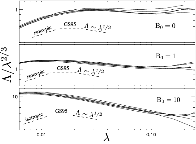
VI. Numerical evidence of interaction weakening
In GS95 turbulent non-linear interactions are strong and the cascading happens fast. In this approach the Kolmogorov’s spectral slope is expected. In order to explain shallower slopes Boldyrev [14] conjectured that interaction is depleted in strong anisotropic turbulence by a factor which is similar to that in the Iroshnikov-Kraichnan (IK) model, i.e. . In simulations with real viscosity we obtain MHD dissipation scale which is somewhat larger than hydro dissipation scale , which can be an indication of depletion of interaction. Figs 1 and 2, upper panel, indicate that is approximately 1.3 times larger than , which is consistent with the difference in dissipation scales of Kolmogorov and IK models, assuming the length of the inertial interval of around 7. However, this result can also be explained by the difference in Kolmogorov constant of hydro and MHD turbulence. Indeed, for MHD [12], while for hydro [32], also note that . Thus, this way of proving the weakening of interaction is still controversial.
VII. Alignment Effects.
While most MHD turbulence models use mean-field approach and assume that turbulence is characterized fully by spectrum or structure functions of the fields, i.e. and , recently a considerable attention has been drawn to so-called alignment effects [13, 6, 14]. The alignment effects can be understood, in general, as a property of multi-variate pdf of the fields containing various correlations. The scale-independent alignment effects are not so interesting, because they can only modify the Kolmogorov constant of turbulence, while scale-dependent alignment can, in principle, modify the slope.
Consider the alignment of Alfvén mode when all perturbations are perpendicular to the local magnetic field, i.e. lie in the same plane. For this purpose we use structure functions where vectors are projected on direction where is the direction, connecting two points [6]. While a study a full multivariate PDF could be an overwhelming task, one can introduce a few statistical measures of alignment that could be of interest. Alignment, derived from zeroth order statistical moments: angle alignment,
| (4) |
where is an angle between Elsasser variables perturbations and , another angle alignment,
| (5) |
where is an angle between and . Alignment derived from second order statistical moments, “polarization intermittency” [6]:
| (6) |
imbalance measure
| (7) |
imbalance correlation
| (8) |
velocity and magnetic fields correlation
| (9) |
(we found that is almost constant in our measurements and it will be assumed constant thereafter). and are describing the same effect, namely dynamic imbalance between Elsasser variables and , but in a different way. For independently distributed Gaussian fluctuations one has , .
Physically, one may have only two types of alignment, because there are four variables (two vectors) minus normalization and minus one arbitrary rotation along axis perpendicular to the magnetic field. Let us choose and as two measures of alignment. is interesting, because it is the factor, by which an interaction is reduced in a nonlinear MHD term with respect to mean field estimate of [13]. This quantity, along with , was first measured in numerical simulations by Beresnyak & Lazarian [6]. In the subsequent publication Mason et al. [48] used a second order structure function measure, very similar to , termed “dynamic alignment”
| (10) |
It can be expressed, to a constant, as (since ), i.e. it is a combination of polarization intermittency and imbalance correlation . It is not clear yet, whether intermittent imbalance can reduce interaction in the balanced turbulence. For example, if one estimates energy dissipation as [46], it is insensitive to the dynamic imbalance , to the first order of . But one also may argue that the imbalanced case is more complicated and the interaction is reduced [7, 8]
Numerically speaking, alignment effects were very similar for all sub-Alfvénic and trans-Alfvénic cases77 7 Beresnyak & Lazarian (2006) observed alignment not only in incompressible simulations, but in trans-Alfvenic, trans-sonic compressible simulations as well.. Fig. 4 shows different alignment measures described in this section for M5 (, Elsasser driving). In the middle of the inertial interval alignment factors depend on k as , , , , , . Note, that DA is short of the dependence predicted for “alignment angle” in Boldyrev [14]. The alignment dependence in the velocity-driven, M4 simulation is somewhat different: , , , , , . If one wanted to explain the difference in slopes between M4 and M5 (, Fig 2) by the difference in DA slopes (according to Boldyrev [14] the slope adds to the spectral slope), such an explanation would be impossible. On the other hand, M4 and M5 are significantly differ by , which suggests that shallow slopes are primarily due to imbalance.

M3 (, velocity driven) simulation show alignment effects which are similar to M4. This directly contradicts to the prediction in Boldyrev [14], that the alignment is a function of , as we observe essentially the same alignment in simulations with and (see also Fig. 6). We therefore conclude that the alignment is an intermittency effect88 8 An intermittency correction is usually written as a function of the ration of the scale in question to the outer scale, e.g. , where is the intermittency correction. In our case we also see that the alignment is a function of . that accumulates along the cascade, rather than being determined rigidly by as in Boldyrev [14]. Alternatively, the alignment could be a natural feature of the nonlocal energy transfer. This calls for further investigation.
VIII. Other hints on nonlocality.
In the sub-Alfvénic turbulence, the properties are well-represented by Elsasser variables and, if we assume locality of interaction of and , the properties of and are supposed to be identical. However, we observed notable differences even after large statistical averaging. Namely, the magnetic energy was higher than kinetic energy in subAlfvénic runs M4 and M5. The last case, which was driven by Elsasser variables, show 50% magnetic energy excess on large scales and around 20% on small scales. This so-called residual energy which was proposed to have “-2” spectrum scaling [51] but was somewhat shallower than “-2” in this Elsasser driven run. Other runs did not show any regular scaling for residual energy. For example, statistically isotropic MHD turbulence M2 show dominance of kinetic energy on large scales (which is typical for MHD turbulence driven with velocity on outer scale), but on small scales magnetic energy dominates (which is typical for almost any driven MHD turbulence). This reinforces our conjecture that currently available 3D MHD simulations do not yet exhibit inertial ranges and the flat portion of the spectrum can not be considered a part of the inertial range of local Kolmogorov-type turbulence until a number of other conditions are satisfied, among which is an equipartition between spectral kinetic and magnetic energies.
IX. Discussion
IX.1. Theory
The nature of the turbulent cascade and the slope of the spectrum of fluctuations is a central issue of turbulence and has been discussed in a majority of papers devoted to turbulence theory and numerics. The hydrodynamic isotropic turbulence has its ‘‘Standard Model’’ which is based on Kolmogorov’s assumption of self-similarity 99 9 This assumption is not precisely satisfied because of so-called intermittency. The most popular descriptions of intermittency are probabilistic models (Obukhov 1962, Kolmogorov 1962, She & Leveque 1994). They give corrections to spectral slopes and higher-order scaling exponents assumed in self-similar model and Kolmogorov’s “-4/5 law”:
| (11) |
Assuming similarity one obtains the second order structure function slope of which correspond to spectral slope of . In MHD, relations, similar to Kolmogorov’s “-4/5 law”, exists, e.g.,
| (12) |
(Chandrasekhar 1951, Politano & Pouquet 1998)1010 10 for statistical isotropy and isotropic structure function or for cylindrical symmetry and perpendicular structure function, e.g. in turbulence with strong mean field.. However, in MHD case, this does not directly hints on scalings for and it is not clear which similarity hypothesis has to be adopted. A nice demonstration of this is to apply the aforementioned exact relations to the case of weak turbulence, where, in the ansatz of three-wave interaction, one has to obtain (anisotropy is defined as a ratio of parallel scale to perpendicular scale ), which is very much unlike the Kolmogorov similarity hypothesis. Thus, the spectral slope scalings are still uncertain, which stimulates further research in this field, including attempts to measure the slope numerically.
The nonlocality of turbulent energy transfer has been claimed in quite a few publications. In the discussion of this numerical work we will mention the most relevant ones and defer more exhaustive discussion to future review papers.
It was suggested in Gogoberidze [29] that in MHD turbulence with strong mean field the nonlinear interaction could be nonlocal, with outer scale perturbations decorrelating high-frequency interacting eddies, leading to IK-type [36, 41] interaction weakening and spectrum. However, in aforementioned model the energy cascading itself is local 1111 11 In a sense that is used, see also §2. and is performed by high-frequency eddies, i.e. there is no energy transfer from large scales directly to small scales. We conclude that this model can not explain the lack of bottleneck effect, observed in simulations.
In a recent model of imbalanced MHD turbulence [7] the eddies of the dominant component on a certain scale are aligned not with respect to the local magnetic field on the same scale as in Cho & Vishniac [22] (balanced turbulence), but with respect to magnetic field on some larger scale. One may speculate that even in the balanced case the dynamic imbalance can cause polarization alignment, or, more likely, that these effects are interrelated. While Beresnyak & Lazarian [7], by itself, is a mean field model and reproduce locality, “-5/3” spectrum and “2/3” anisotropy of GS95 in the balanced limit, its future extentions to include local imbalance and polarization alignment seems promising.
Does the hypothesis of Boldyrev (2006) that the and alignment is limited by field wandering is justified from theory ground? In a little thought experiment one can imagine a perfectly aligned state where the magnitudes of and are equal. This is a case of a perfect imbalance and also an exact solution of MHD equations. Such a state will propagate without distortion, in other words, no de-alignment is going to happen, although this state certainly has some level of field wandering. This thought experiment hints that the hypothesis of and alignment being limited by field wandering directly contradicts MHD equations. The effect of local imbalance, therefore, has to be treated in a more complicated way. Fig. 6 shows a comparison between field wandering () and “dynamic alignment” in transAlfvénic M3 and subAlfvénic M4. We see that in subAlfvénic case the dynamic alignment is an order of magnitude off the , which is in contrast with Boldyrev [14] which suggest that .

IX.2. Previous numerical work
The study of weakly compressible MHD turbulence by Haugen et al. [33], Haugen et al. [34] revealed some difference in bottleneck effect in hydro and MHD cases, although the authors reported bottleneck behaviour as “very similar”. The difference was small, possibly, due to adopted first order viscous and resistive dissipation. Aforementioned work, however, used finite-difference code and, inadvertently, the numerical dissipation had a different character in MHD and hydro simulations, which precluded a rigorous comparison. Nevertheless, we can say that it is consistent with what we see in our incompressible simulations.
Biskamp et al. (1998) studied two-dimensional MHD and EMHD turbulence. They noticed that both MHD and EMHD cases have an unusual nonlocal bottleneck effect, which appeared differently depending on numerical resolution. It is possible that spectral flattening from such an effect can be perceived as a ”false” inertial interval and lead to an incorrect estimate of the slope. Although there had been much discussion on the analogy between two-dimensional MHD turbulence and MHD turbulence with strong mean field, the predominant picture is that Alfvénic turbulence is essentially three-dimensional (GS95, Cho & Vishniac 2000, Maron & Goldreich 2001, Cho et al. 2002).
Yousef et al. (2007) claimed that in the statistically isotropic MHD turbulence (similar to our simulation M2) one has a folded magnetic field structures that directly non-locally interact with outer-scale motions. They concluded that one can not use Kolmogorov argumentation because of this nonlocality. We, however, belive, that Kraichnan’s argumentation regarding the dominance of local mean field, i.e. the Alfvén effect, is correct even in the case of . This is somewhat hard to demonstrate in 3D numerics, however, because for there is a transition region between outer scale and inertial interval where kinetic energy dominates and the magnetic spectrum is very flat, i.e., there is no clear dominance of the large-scale magnetic field. Also the use of first-order (natural) viscosity in aforementioned three-dimensional simulations made the inertial range very short, which created an illusion of a universal folded magnetic field structure.
Alexakis et al. (2005a, 2005b) used a specific numerical tool to quantify the transfer of energy between scales in both hydro and MHD turbulence. They claimed that MHD case is somewhat nonlocal. However, the more radical claim is that the hydro cascade and the larger part of MHD cascade is extremely local, i.e. the energy is not transferred between k and 2k, as in Kolmogorov model, but instead between k and where is determined by outer scale, which breaks self-similarity. We find these results rather puzzling and defer discussion until independent confirmation is available. Until then, we assume that Kolmogorov picture is roughly appropriate for isotropic hydrodynamic turbulence with large inertial range.
IX.3. Implications for astrophysical turbulence
Realistic astrophysical turbulence is, in general, compressible. The examples of weakly compressible flows are the quiet convection in main sequence stars and turbulence in very hot intracluster gas. The turbulence in most of the Interstellar Medium, however, is strongly compressible, due to effective cooling. This raises the question of to what extend the results of incompressible simulations are applicable to astrophysics. Intuitively, one could expect that weak small-amplitude Alfvén and slow-mode turbulent perturbations should be nearly incompressible. The question is how to deal with the fast mode and large-amplitude MHD turbulence in compressible fluids.
The coupling of Alfvénic motions and compressible motions is a difficult subject. Theoretical arguments that fast, slow and Alfvén modes may create independent energy cascades were provided in GS95, Lithwick & Goldreich (2001) and Cho & Lazarian (2003). These arguments were applicable to strong Alfvénic turbulence1212 12 The more detailed study (Chandran 2005) of weak Alfvénic turbulence in a pressure-less medium showed that the interactions between the fast and Alfvénic modes may be significant in a certain regions of k-space.. Cho & Lazarian (2002, 2003) numerically demonstrated that for even for appreciable Mach numbers (up to 10), the properties of Alfvénic modes (scalings and anisotropy) were similar to those in incompressible simulations1313 13 Density perturbations, which are absent in incompressible flows, are definitely affected by compressible motions. However, Beresnyak et al. (2005) found that the structure of logarithm of density reveal scale-dependent anisotropy, similar to GS95 law. This presumes that a significant fraction of density structures are created by shearing by Alfvénic perturbations.. They also showed that the decay time for the Alfvénic modes is fast and not mediated through coupling with compressible motions, which used to be the common wisdom at the time of the study. The effect of scale-dependent polarization alignment, a characteristic of Alfvénic cascade discussed in this paper, happen to be present in both compressible and incompressible MHD simulations (Beresnyak & Lazarian 2006). While the extend to which strong shocks can modify the Alfvénic cascade deserves more study, the arguments above make us confident that the studies of incompressible turbulence are of primary importance to understand astrophysical turbulence.
There is another issue, which is frequently ignored when one compares numerical MHD with interstellar turbulence. If magnetic fields are perfectly frozen into the fluid, turbulence creates multiple small-scale current sheets which are difficult to dissipate. Within such zones the frozen-in condition is no longer valid and magnetic reconnection takes place (see Biskamp 2000, Priest & Forbes 2000, Bhattacharjee 2004, Zweibel & Yamada 2009). The Lundquist number that characterizes how well magnetic fields are frozen in ( is the scale of the current sheet and is magnetic diffusivity), is very high, e.g. , for most astrophysical fluids and is fairly low, e.g. , for MHD simulations. If magnetic reconnection in astrophysics depends on , this presents not only a problem for most of MHD simulations, e.g. simulations of dynamo, molecular clouds, accretion disks, but also means that the numerical results on turbulent scalings may not be trusted. We believe that the extensive observational data suggests that magnetic reconnection is fast. Also, a model predicting fast reconnection in turbulent fluids, Lazarian & Vishniac (1999), has been successfully tested in Kowal et al. (2009). This gives additional support to numerical testing of astrophysical turbulence.
The slopes and turbulence anisotropies are important for a variety of astrophysical phenomena. For instance, scattering and turbulent acceleration of cosmic rays depends on the scaling of MHD turbulence (see Chandran 2000, Yan & Lazarian 2002, 2004). So does the perpendicular diffusion of cosmic rays and heat transport in plasmas (Narayan & Medvedev 2001, Lazarian 2006). Naturally, it is important to establish the true scalings of MHD turbulence. This paper testifies that a higher resolution numerical simulations are required for accurate testing of the present and future MHD turbulence models.
X. Conclusions
We conclude that although the Kolmogorov-like Goldreich-Sridhar (GS95) model is appealing, simple and captures some essential physical properties of the strong MHD turbulence, such as scale-dependent anisotropy, it should be amended to explain cascade nonlocality and scale-dependent alignment effects. How to achieve this is the issue of the future research, as we demonstrate that the existing attempts to improve GS95 do not agree well with the presented numerical simulations. In addition, we issue a note of warning that the numerical measurements of the spectral slope that served as a motivation for many of theoretical studies are unlikely to represent the true theoretical slopes due to the non-locality of MHD cascade.
References
- [1] Alexakis, A., Mininni, P. D., & Pouquet, A. 2005, Phys. Rev. Lett., 95, 26, 264503
- [2] Alexakis, A., Mininni, P. D., & Pouquet, A. 2005, Phys. Rev. E, 72, 4, 046301
- [3] Armstrong, J. W., Rickett, B. J., & Spangler, S. R. 1995, ApJ, 443, 209
- [4] Balbus, S. A., & Hawley, J. F. 1991, ApJ, 376, 214
- [5] Beresnyak, A., Lazarian, A., & Cho, J. 2005, ApJ, 624, 93L
- [6] Beresnyak, A., Lazarian, A. 2006, ApJ, 640, L175
- [7] Beresnyak, A., Lazarian, A. 2008, ApJ, 678, 961
- [8] Beresnyak, A., Lazarian, A. 2009, ApJ submitted, arXiv:0904.2574
- [9] Bhattacharjee, A. 2004, ARA&A, 42, 365
- [10] Biskamp, D., Schwarz, E., & Celani, A. 1998, Phys. Rev. Lett. 81, 4855
- [11] Biskamp, D. 2000, Magnetic Reconnection in Plasmas (Cambridge, UK:Cambridge University Press)
- [12] Biskamp, D. 2003, Magnetohydrodynamic Turbulence. (Cambridge: CUP)
- [13] Boldyrev, S. 2005, ApJ, 626, L37
- [14] Boldyrev, S. 2006, Phys. Rev. Lett., 96, 115002
- [15] Chandran B.D.G., Phys. Rev. Lett., 85 (22), 4656-4659 (2000)
- [16] Chandran, B. D. G. 2005, Physical Review Letters, 95, 265004
- [17] Chandrasekhar, S. 1951, Proc. Roy. Soc. London, Ser. A, 204, 435
- [18] Chandrasekhar, S. 1960, Proceedings of the National Academy of Science, 46, 253
- [19] Cho, J., & Lazarian, A. 2002, Phys. Rev. Lett., 88, 24, 5001
- [20] Cho, J., & Lazarian, A. 2003, MNRAS, 345, 325
- [21] Cho, J., Lazarian, A., & Vishniac, E. T. 2002, ApJ, 564, 291
- [22] Cho, J. & Vishniac, E. 2000, ApJ, 539, 273
- [23] Crovisier, J., & Dickey, J. M. 1983, A&A, 122, 282
- [24] Dobler, W., Haugen, N. E., Yousef, T. A., Brandenburg, A. 2003, Phys. Rev. E, 68, 026304
- [25] Dobrowolny, M., Mangeney, A., & Veltri, P. 1980, Physical Review Letters, 45, 144
- [26] Elmegreen, B. G., & Scalo, J. 2004, ARA&A, 42, 211
- [27] Galtier, S., Nazarenko, S.V., Newel, A.C., Pouquet, A., J. Plasma Phys., 63, 447 (2000)
- [28] Galtier, S., Nazarenko, S., Newell, A., & Pouquet, A., ApJ, 564, L49 (2002)
- [29] Gogoberidze, G. 2007, Phys. Plasmas, 14, 022304
- [30] Goldreich, P., & Sridhar, S. 1995, ApJ, 438, 763
- [31] Falkovich, G. 1994, Phys. of Fluids, 6, 1411
- [32] Frisch, U. 1995, Turbulence, the legacy of A.N.Kolmogorov, Cambridge: CUP
- [33] Haugen, N. E., Brandenburg, A., Dobler, W. 2003, ApJ, 597, L141
- [34] Haugen, N. E., Brandenburg, A., Dobler, W. 2004 Phys. Rev. E, 70, 016308
- [35] Higdon, J. C. 1984, ApJ, 285, 109
- [36] Iroshnikov, P.S. 1963, AZh, 40, 742
- [37] Kaneda, Y., Ishihara, T., Yokokawa, M., Itakura, K., & Uno, A. 2003, Phys. Fluids, 15, L21
- [38] Kolmogorov, A. 1941, Dokl. Akad. Nauk SSSR, 31, 538
- [39] Kolmogorov, A.N., J. Fluid Mech. 13, 82 (1962)
- [40] Kowal, G., Lazarian, A., Vishniac, E., Otmianowska-Mazur K. 2009, ApJ, submitted, arXiv:0903.2052
- [41] Kraichnan, R.H. 1965, Phys. Fluids,8, 1385
- [42] Kritsuk, A.G., Norman, M. L., Padoan, P., Wagner, R. 2008, ApJ, 665, 416
- [43] Lazarian, A. 2009, Space Science Reviews, 143, 357
- [44] Lazarian, A., & Vishniac, E. T. 1999, ApJ, 517, 700 (LV99)
- [45] Lazarian, A. 2006, ApJ, 645, 25L
- [46] Lithwick, Y., Goldreich, P., & Sridhar, S. 2007, ApJ, 655, 269
- [47] Maron, J., & Goldreich, P. 2001, ApJ, 554, 1175
- [48] Mason, J., Cattaneo, F., Boldyrev, S., 2006, Phys. Rev. Lett., 97, 255002
- [49] McKee, C. F., & Ostriker, E. C. 2007, ARA&A, 45, 565
- [50] Müller, W.-C., & Biskamp, D. 2000, Physical Review Letters, 84, 475
- [51] Müller, W.-C. & Grappin, R. 2005, Phys Rev Lett 95, 114502
- [52] Monin, A.S., Yaglom, A.M. 1975, Statistical Fluid Mechanics: Mechanics of Turbulence, NY: Dover
- [53] Montgomery, D., & Turner, L. 1981, Physics of Fluids, 24, 825
- [54] Narayan, R. & Medvedev, M. V. 2001, ApJ, 562, 129L
- [55] Ng, C. S., & Bhattacharjee, A. 1996, ApJ, 465, 845
- [56] O’dell, C. R., & Castaneda, H. O. 1987, ApJ, 317, 686
- [57] Obukhov, A. M. 1962, J. of Geophys. Res., 67, 3011
- [58] Parker, E. N. 1966, ApJ, 145, 811
- [59] Politano, H.,& Pouquet, A. 1998, Phys. Rev. E, 57, 21
- [60] Priest, E., & Forbes, T. 2000, Magnetic Reconnection, (Cambridge, UK:Cambridge University Press)
- [61] She, Z.-S. & Leveque, E., Phys. Rev. Lett., 72, 336 (1994)
- [62] Shebalin, J. V., Matthaeus, W. H., & Montgomery, D. 1983, Journal of Plasma Physics, 29, 525
- [63] Sridhar, S., & Goldreich, P. 1994, ApJ, 432, 612
- [64] Stone, J. M., Ostriker, E. C., & Gammie, C. F. 1998 ApJ, 508, L99
- [65] Velikhov, E.P. 1959, Soviet Phys.–JETP Lett, 36, 1398
- [66] Yan, H., & Lazarian, A. 2002, Physical Review Letters, 89, 1102
- [67] Yan, H., & Lazarian, A. 2004, ApJ, 614, 757
- [68] Yousef, T. A., Rincon, F., & Schekochihin, A. A. 2007, J. Fluid Mech. 575, 111
- [69] Zweibel, E., & Yamada, M. 2009, ARA&A, in press