KUNS-2170
Instabilities of Kerr-AdS Spacetime
Keiju Murata
Department of Physics, Kyoto University, Kyoto 606-8501, Japan
e-mail:murata@tap.scphys.kyoto-u.ac.jp
August 24, 2026
We study gravitational perturbations of the Kerr-AdS spacetime with equal angular momenta. In this spacetime, we found the two kinds of classical instabilities, superradiant and Gregory-Laflamme instabilities. The superradiant instability is caused by the wave amplification via superradiance, and by wave reflection due to the potential barrier of the AdS spacetime. The Gregory-Laflamme instability appears in Kaluza-Klein modes of the internal space and breaks the symmetry . Taken into account these instabilities, the phase structure of Kerr-AdS spacetime is revealed. The implication for the AdS/CFT correspondence is also discussed.
1 Introduction and Summary
Recently, AdS black holes in compactified type IIB supergravity have attracted much interest because they describe strongly coupled thermal super Yang-Mills theory via AdS/CFT correspondence [1, 2, 3, 4]. Especially, phase transitions of dual gauge theory are identified with instabilities of AdS black holes and understanding of stability of AdS black holes is important to reveal the strongly coupled gauge theory.
The stability of Schwarzschild-AdS black holes has been shown in [5, 6, 7, 8, 9]. However, in the case of Kerr-AdS black holes, we can expect an instability called superradiant instability. The perturbation of Kerr-AdS black holes can be amplified by superradiance at the horizon. On the other hand, at the infinity, the amplified perturbation will be reflected by the potential barrier of the AdS spacetime. This will be amplified at the horizon again. By repetition of this mechanism, the initial perturbation can grow exponentially and Kerr-AdS black holes become unstable. The superradiant instability is physically reasonable, but, practically, it is difficult to find the instability by gravitational perturbation because of the difficulty of separation of perturbation equations. Nevertheless, in some special cases, there are several works on the stability of Kerr-AdS black holes. In the case of 4-dimensional Kerr-AdS spacetime, the superradiant instability has been found [10, 11]. In , the same instability of Kerr-AdS black holes with equal angular momenta has been shown to exist [13]. In the case of -dimensional Kerr-AdS black hole with one rotating axis, it has been shown that the superradiant instability appears in the tensor type perturbation [14, 15]. However, there is no work for the stability analysis of five-dimensional Kerr-AdS black holes (except for a massless Kerr-AdS black holes [16] or a scalar field perturbation [17]). To get relevant results for the AdS5/CFT4 correspondence, we need to study the instability of five-dimensional Kerr-AdS black holes. It is difficult to study the stability of the general Kerr-AdS5 spacetime. However, for equal angular momenta case, spacetime symmetry of Kerr-AdS5 black hole is enhanced and the separation of gravitational perturbation equations can be possible [18, 21, 19, 20]. One of our purposes is to find the superradiant instability of five-dimensional Kerr-AdS black holes with equal angular momenta.
The superradiant instability is caused by property of rotating AdS black holes and information of the internal space is not so important for superradiant instability. However, if the internal space is taken into account, we can find another type of instability, called Gregory-Laflamme instability. Originally, the Gregory-Laflamme instability has been found in the black brane solution [22, 23, 24], but, in the Schwarzschild-AdS spacetime, the situation can be similar to the black brane system. If the horizon radius is much smaller than radius of , the internal space may be considered as . Then, we can consider Sch-AdS spacetime as a black brane and the Gregory-Laflamme instability may appear in Kaluza-Klein modes. The Gregory-Laflamme instability of Schwarzschild-AdS spacetime has been already found in [25]. In this paper, extending their work, we study the Gregory-Laflamme instability of Kerr-AdS spacetime.
We will take into account Gregory-Laflamme and superradiant instabilities and reveal the phase structure of Kerr-AdS spacetime. There are two kinds of instabilities in the Kerr-AdS spacetime. Thus, we can expect that this spacetime has rich phase structure and it will be useful to find the evidence of the AdS/CFT correspondence.

The organization and summary of this paper is as follows. In section 2, we introduce Kerr-AdS spacetimes with equal angular momenta. Especially, the spacetime symmetry is studied. We shall see that the symmetry is in the case of equal angular momenta. In section 3, we study the gravitational perturbation of Kerr-AdS5 spacetime neglecting the Kaluza-Klein modes of the internal space . We can get the master equations which are relevant for the superradiant instability. These equations are solved numerically and we find the onset of superradiant instabilities given by , where is angular velocity of horizon and is curvature scale of AdS spacetime. In section 4, we study Gregory-Laflamme instability of Kerr-AdS spacetime. We consider the gravitational perturbation including Kaluza-Klein modes in order to see the Gregory-Laflamme instability and get the ordinary differential equations in which three variables are coupled. These equations are solved numerically and we find the Gregory-Laflamme instability. In section 5, we reveal the phase structure of Kerr-AdS spacetime taking into account superradiant and Gregory-Laflamme instabilities. The result is in Figure.1, and are angular velocity and temperature of Kerr-AdS5 black holes. In Figure.1, and are normalized by the curvature scale of the AdS spacetime, . The solid and dashed lines are onset of the Gregory-Laflamme and superradiant instabilities, respectively. These lines cross each other and we can see five phases in this diagram. In the “Stable” region, Kerr-AdS black holes are stable. In the “SR” and “GL” region, black holes are unstable against superradiant and Gregory-Laflamme instabilities, respectively. In “SR&GL” region, black holes are unstable against both of them. In “No Black Holes” region, there is no black hole solution. The final section is devoted to the conclusion.
2 Kerr-AdS5 black hole in Type IIB Supergravity
2.1 Kerr-AdS spacetime with equal angular momenta
In this section, we introduce Kerr-AdS5 spacetime as a solution of type IIB supergravity. The equations of motion of type IIB supergravity are given by
| (2.1) | |||
| (2.2) |
where . The form is RR 5-form satisfying and . We concentrate on the metric and RR 5-form field in type IIB supergravity, while other components, such as dilaton, NSNS 3-form, RR 1-form and 3-form, have been set to be zero. We will consider Kerr-AdS spacetime which is a solution of (2.1) and (2.2). The Kerr-AdS5 spacetime can have two independent angular momenta generally, but, for simplicity, we will consider the case of equal two angular momenta. Then, the spacetime symmetry is enhanced and stability analysis will be possible. The metric of Kerr-AdS spacetime with equal angular momenta is given by11 1 To obtain this metric from Kerr-AdS5 spacetime given in [26, 27, 28, 29], we need some coordinate transformation and redefinition of a parameter. These are summarized in appendix A.
| (2.3) |
where is defined by
| (2.4) |
Then, RR 5-form is
| (2.5) |
where is volume form of and is volume form of AdS5 part of (2.3). Because of the relation, , the form satisfies the self dual condition. In (2.3), we have defined the invariant forms of as
| (2.6) |
where , , . It is easy to check the relation . The dual vectors of are given by
| (2.7) |
and, by the definition, they satisfy .
The horizon radius can be determined by . The angular velocity of Kerr-AdS back hole is given by
| (2.8) |
For existence of horizon, the angular velocity has the upper bound,
| (2.9) |
In term of and , the two parameters in the metric (2.3) can be rewritten as
| (2.10) |
We will use parameters mainly.
2.2 Spacetime Symmetry
Now, we study the symmetry of (2.3). It will be important for separation of variables of the gravitational perturbation equations in section 3 and 4. Apparently, the metric (2.3) has the time translation symmetry and symmetry comes from part of (2.3). Additionally, the spacetime has the symmetry characterized by the Killing vectors :
| (2.11) |
The symmetry can be explicitly shown by using the relation , where is a Lie derivative along the curve generated by the vector field .
From the metric (2.3), we can also read off the additional symmetry, which keeps the part of the metric, and is generated by . The generator satisfies and and, thus, . Therefore, the symmetry of Kerr-AdS spacetime with equal angular momenta becomes .
For later calculations, it is convenient to define the new invariant forms
| (2.12) |
Then, the dual vectors for are
| (2.13) |
By making use of these forms, the metric (2.3) can be rewritten as
| (2.14) |
We will use this expression in the following sections.
3 Superradiant Instability of Kerr-AdS black holes
In the following sections, we will study the stability of Kerr-AdS spacetime with equal angular momenta (2.3). In this spacetime, we can expect two kinds of instabilities. One of them is the superradiant instability which is caused by the wave amplification via superradiance, and by wave reflection due to the potential barrier of the AdS spacetime. This instability should be seen, even if Kaluza-Klein modes are neglected. The other instability is the Gregory-Laflamme instability which is instability of the internal space , that is to say, the Gregory-Laflamme instability is instability of Kaluza-Klein modes. First, we shall see the superradiant instability of Kerr-AdS5 spacetime in this section.
3.1 Perturbation equations and separability
To see the superradiant instability, we can neglect Kaluza-Klein modes of . In addition, we will consider only metric fluctuation on the AdS5 part of the spacetime, that is,
| (3.1) |
where are indexes on AdS5 and is volume form of . For the perturbations, the equation (2.2) is trivially satisfied and equation (2.1) becomes
| (3.2) |
where is perturbation of the Einstein tensor of five-dimensional metric , which is defined by
| (3.3) |
where denotes the covariant derivative with respect to and . Tensors and are Ricci tensor and Ricci scalar of . We take AdS5 part of (2.14) as a background metric . The equation (3.2) is nothing but the perturbation of five-dimensional Einstein equations with the negative cosmological constant.
The perturbation equation (3.2) is a partial differential equation of . However, in previous works [30, 18, 19, 21], it was shown that the perturbation equations can be reduced to ordinary differential equations by focusing on the symmetry of the background spacetime, . Here, we will briefly review these works.
Let us define the two kinds of angular momentum operators
| (3.4) |
where and . They satisfy commutation relations
| (3.5) |
where and are antisymmetric tensors which satisfy . The Casimir operators constructed by and are identical and we define . The symmetry group, is generated by and . Here, we should notice the fact
| (3.6) |
It means that and have charges and . Since operators , and commute each other, these are simultaneously diagonalizable. The eigenfunctions are called Wigner functions defined by
| (3.7) |
where indexes and are defined for and . The following relations are useful for later calculations
| (3.8) |
where we have defined and . From this relation, we get the differential rule of the Wigner function as
| (3.9) |
where we have defined and .
Now, we consider the mode expansion of . The metric perturbations can be classified into three parts, where and . They behave as scalar, vector and tensor for coordinate transformation of , respectively. The scalar can be expanded by Winger functions immediately as
| (3.10) |
Here, we have omitted the indexes because the differential rule of Wigner function (3.9) cannot shift and therefore the modes with different eigenvalues are trivially decoupled in the perturbation equations.
To expand the vector part , we need a device. First, we change the basis to , that is where . Then, because is scalar, we can expand it by the Wigner function as
| (3.11) |
In the expansion of , and , we have shifted the index of Wigner functions, for example, has been expanded as . The reason is as follows. The invariant forms and have the charge and , respectively (see Eq. (3.6)), while the Wigner function has the charge (see Eq. (3.7)). Therefore, by shifting the index , we can assign the same charge to , and in Eq. (3.11).
The expansion of tensor part can be carried out in a similar way as
| (3.12) | |||||
To assign the same charge to each term, we have shifted the index of Wigner functions.
Substituting Eqs. (3.10), (3.11), (3.12) into the perturbation equations (3.2), we get the equations for each mode labelled by , , . Because of symmetry, different eigenmodes cannot appear in the same equation.
It is interesting that we can find master variables from above information. First, we should notice that coefficients of the expansion have different indexes and, therefore, coefficients of components , and are restricted as follows:
From this table, we can see that, in mode, there is only one variable , respectively. Therefore, the modes always reduce to a single master equation. We will study the stability of these modes. In fact, modes also reduce to a single master equation. The stability of modes are studied in appendix B and we will see that these modes are irrelevant to see the onset of the superradiant instability.
3.2 Master Equations
We will derive the master equation for modes. Because of the relation , we will consider modes only. Then, we can set as
| (3.13) |
where . This field is gauge invariant. We substitute Eq. (3.13) into Eq. (3.2) and use the differential rule of Wigner functions (3.9). Then, component of (3.2) is given by
| (3.14) |
This equation can be rewritten as
| (3.15) |
where we have introduced the new variable,
| (3.16) |
and the tortoise coordinate,
| (3.17) |
The function and potential are given by
| (3.18) |
and
| (3.19) |
We can obtain the asymptotic form of and as
| (3.20) |
and
| (3.21) |
where is the angular velocity of the horizon which is defined in Eq. (2.8). Therefore, the asymptotic form of the solution of master equation (3.15) becomes
| (3.22) |
We will solve (3.15) numerically and show the superradiant instability.
3.3 Stability analysis
3.3.1 A Method to Study the Stability
We will find the instability by shooting method. Then, since the master equation (3.15) is not self adjoint form, we should put () and there are two shooting parameter, and . However, if the purpose is to find the onset of instability, the number of shooting parameter can be reduced to one [31, 13, 21].
We have separated the time dependence as in (3.13). Therefore, unstable mode satisfies . Thus, the boundary condition for regularity at the horizon becomes
| (3.23) |
Then, the general form of wave function at infinity becomes
| (3.24) |
where are constants. For regularity at infinity, the condition must be satisfied. Therefore, the boundary conditions which unstable mode satisfies are
| (3.25) |
Now, we consider the marginally stable mode. then, we can set . In this case of , Wronskian of is conserved, that is,
| (3.26) |
for any and . We take and . Then, from Eq. (3.26), we can get the relation,
| (3.27) |
where we have used the asymptotic form of (3.23) and (3.24). To avoid divergence at infinity, must be satisfied. Then, we can get
| (3.28) |
Therefore, equation which we should solve is
| (3.29) |
where
| (3.30) |
The boundary condition can be obtained by substituting into (3.30) and it is given by
| (3.31) |
There is only one shooting parameter, , in (3.29).
3.3.2 Limit of Small Kerr-AdS Black Holes
Before the numerical calculation, it is important to solve master equation (3.29) analytically in some limit [32]. It may be useful to check the numerical calculation. We consider Kerr-AdS black holes in the limit of . Then, master equation (3.15) can be solved exactly. The solution which approach to zero at infinity is
| (3.32) |
where is Gauss hypergeometric function. Then, the asymptotic form of becomes
| (3.33) |
For the regularity at horizon, the first term of (3.33) must vanish. Thus, we can get where . This calculation is to see the onset of the instability and the lowest value of is important. The lowest value of is given by
| (3.34) |
Numerical result must approach this value in the limit of .
3.3.3 Onset of superradiant instability
Now, we shall solve (3.29) numerically. Using the Lunge-Kutta algorithm, we integrate the Eq. (3.29) from the horizon to infinity with various . The boundary conditions at the horizon are given by (3.31). Then, the general form of the wave function at infinity is given by (3.24). We can see that, at some value of , the flip the sign. It means that mode exists. We will search such numerically and plot the result in - diagram. The result is in Figure.2. The curves represent borderline of stability and instability of each mode, that is, each mode is stable below the curve, while they are unstable above the curve. From this figure, we can read off that, in the limit of , these curves for each mode approach . This result is consistent for analytical calculation in section 3.3.2. We can also see that, for higher mode, the instability occurs at a lower angular velocity. These curves seem to approach for large . These properties are the same for cases [13].
It is surprising that these results have been already seen in dual gauge theory [34, 33]. In [34], effective mass term for scalar fields of dual gauge theory have been obtained as
| (3.35) |
Because of , if satisfied, is positive for any and . However, if , can be negative for large and modes. Thus, we see that, for , dual gauge theory is unstable and higher mode becomes tachyonic first as increases. These results are the same for superradiant instability of Kerr-AdS5 black holes.

4 Gregory-Laflamme instability of Kerr-AdS spacetimes
4.1 Perturbation Equation
In the previous section, we have seen the superradiant instability of Kerr-AdS spacetime. The superradiant instability breaks the symmetry of Kerr-AdS5. In this section, we will consider the Gregory-Laflamme instability of Kerr-AdS spacetimes. This instability breaks the symmetry of . Thus, we must see the Kaluza-Klein modes of the perturbations which have been neglected in the previous section.
We will consider only the metric fluctuations on the AdS5 part of the spacetime, that is,
| (4.1) |
where is spherical harmonics on which satisfy
| (4.2) |
here is the Laplacian of and . The in (4.1) is the volume form of . Since, in the case of Schwarzschild-AdS, the Gregory-Laflamme instability has been found in these fluctuations [25], the instability of Kerr-AdS must also appear in these fluctuations. Here, we should notice that, in (4.1), depends on the coordinates on . It is essential to see the Gregory-Laflamme instability. Then, from (2.1), we can obtain the perturbation equations as
| (4.3) |
where and is defined in (3.3). From (2.2), we can get
| (4.4) |
where is index on . In the case , (4.4) is trivially satisfied and (4.3) reduces to (3.2). For , (4.4) implies . Then, as a constraint equation of (4.3), we can get transverse condition of as shown in the appendix C. Thus, even for Kaluza-Klein modes, we can use transverse traceless conditions,
| (4.5) |
To separate variables of equations (4.3) and (4.5), we will use the formalism in the section 3.1 again. We can expand by the Wigner function and obtain ordinary differential equations labeled by . We will not study the stability of all modes, but we will consider only mode. The Gregory-Laflamme instability of Schwarzschild-AdS spacetime was found in the s-wave of AdS5 [25] and, thus, we can expect that, in the Kerr-AdS spacetime, the instability appears in most symmetric mode, . The metric perturbation for this mode is given by
| (4.6) |
where we assume that the metric perturbation does not depend on , in order to see the onset of Gregory-Laflamme instability. The stability of mode of this perturbation is shown in Appendix B.1 and, thus, we will consider . We substitute (4.6) into (4.3). Then, from and components of the perturbation equation, we can obtain
| (4.7) |
Now, we introduce dimensionless variables, and , as
| (4.8) |
Hereafter, we put to simplify expressions. Then, the traceless condition can be written as
| (4.9) |
and the -component of transverse condition is
| (4.10) |
where . We can see that, using (4.9) and (4.10), and can be eliminated.22 2 We can eliminate other variables, such as (), (). However, if we eliminate these variables, the singular point will appear at in the resultant equations [25]. The variables () are the best variables for elimination as far as we can see. Then, , and component of (4.3) are given by
| (4.11) | ||||
| (4.12) | ||||
| (4.13) |
We can check that the other components of (4.3) are derived from (4.11), (4.12) and (4.13). There are three degree of freedom in mode.33 3 In the case , the gauge freedom are restored and degree of freedom becomes one as explained in appendix B.1.
4.2 Onset of the Gregory-Laflamme instability
We will solve equations (4.11), (4.12) and (4.13) numerically and see the onset of the Gregory-Laflamme instability. First, we derive the boundary conditions at the horizon. Substituting
| (4.14) |
into (4.11), (4.12) and (4.13), we obtain
| (4.15) |
Free parameters remain. However, we can set by the rescale of . Hence, parameters which we should set at horizon are . On the other hand, at , the growing mode of becomes
| (4.16) |
Thus, for large , we can get the coefficients of the growing modes approximately as
| (4.17) |
These must be zero at infinity44 4 For , is not singular even if , but for the regularity of , we need . .
Now, we can start the numerical integration. We solve (4.11), (4.12), (4.13) from to by the Runge-Kutta algorithm. Input parameters are and we can get at . For fixed , we look for which satisfy by the Newton-Raphson method. We repeat this procedure with various . The result is given in Figure. 3. These lines have maximum value and approach for . We can see that mode is relevant for the onset of the Gregory-Laflamme instability. It is remarkable that onset line of Gregory-Laflamme and superradiant instabilities intersect each other. Thus, both of the instabilities can appear in Kerr-AdS spacetimes. In the limit of , we can read off the onset of the instability as . It is consistent with the instability of Schwarzschild-AdS spacetimes [25].

5 Phase structure
In this section, taking into account superradiant and Gregory-Laflamme instabilities, the phase structure of the Kerr-AdS spacetime is revealed. Here, we need some comments on the stability analyses performed in section 3 and 4. We studied some specific modes and found instabilities. However, we did not study all modes of perturbations and, strictly speaking, onsets of superradiant and Gregory-Laflamme instabilities can be changed by all modes analysis. To make sure that the onset of instabilities that we derived gives a true onset of instability, we studied the stability of , modes in Appendix B.3. As the result, we found the instability whose onset is given by . This result suggest that mass term of graviton lifts up the onset of instability and these are not relevant to see the onset of superradiant instability. The result of Appendix B.3 also suggests that the Gregory-Laflamme type instability is not found in higher modes in AdS5 part of spacetime. Because of above reason, we regard the result derived in section 3 and 4 as a true onset of instabilities and reveal the phase structure of Kerr-AdS spacetimes.
Until previous section, we have been using parameters . However, for comparison with the gauge theory, the horizon radius is not a good parameter because is not defined in the gauge theory. Therefore, we see the phase diagram by thermodynamical parameters, the temperature and angular velocity . The temperature is defined by
| (5.1) |
Using this equation, we can map Figure.3 onto - diagram. The result is given in Figure.1. The solid and dashed lines are the onset of Gregory-Laflamme and superradiant instabilities, respectively. These lines cross each other and we can see five phases in this diagram. In the “Stable” region, Kerr-AdS black holes are stable. In the “SR” and “GL” region, black holes are unstable against superradiant and Gregory-Laflamme instabilities, respectively. In “SR&GL” region, black holes are unstable against both of them. In “No Black Holes” region, there is no black hole solution.
To get this phase diagram, we need some attentions. In Figure.4, we plot the temperature as a function of . In the case of , there are two giving the same temperature. We will call these phases as small and large black hole phases. There is no one-to-one correspondence for and . Since the Gregory-Laflamme instability appears in the small black hole phase, we chose the small black hole phase to depict the phase diagram. We can also see that the temperature has minimal value . The “No Black Holes” phase in Figure.1 comes from this bound. In the case of , the temperature has no minimal value, but it is bounded by . For , becomes zero at some value of . Thus, “No Black Holes” phase is vanishing for in Figure.1. The line in Figure.3, has been mapped onto a ray of and .

6 Conclusions and Discussions
We have studied gravitational perturbations of Kerr-AdS spacetimes with equal angular momenta. First, we studied the stability of Kerr-AdS5 neglecting Kaluza-Klein modes and found the superradiant instability. We could see that the onset is given by . We also studied the stability including Kaluza-Klein modes of and found the Gregory-Laflamme instability. From these results, we made out the phase diagram of Kerr-AdS spacetime in Figure.1 and found five phases in this diagram.
It is surprising that superradiant and Gregory-Laflamme instabilities can be understood by the dual gauge theory. In the dual gauge theory, the angular velocity of the horizon is regarded as a chemical potential [26, 33, 34]. It has been shown that, for , the gauge theory is unstable and higher mode becomes tachyonic first as increases [34]. In gravity theory, we found same property, that is, we can see that, from Figure.2, higher mode becomes unstable first as increases. This remarkable coincidence of gravity and gauge theories gives a strong evidence for the AdS/CFT correspondence.
There are also several works on the Gregory-Laflamme instability from the gauge theory point of view [35, 36, 37, 38]. Especially, in [38], SYM on , which is dual to the Schwarzschild-AdS spacetime, is studied with weak ’t Hooft coupling. In their work, for high temperature, they found a new saddle point in which R-symmetry is spontaneously broken and symmetry is remained. The R-symmetry in the gauge theory corresponds to the symmetry of internal space in the dual gravity theory and, thus, this appearance of the new saddle point was identified to the Gregory-Laflamme instability. For the Kerr-AdS spacetime, our result of Figure.1 gives a prediction for the phase structure of the gauge theory. However, unfortunately, there is no work for the Gregory-Laflamme instability in the view of gauge theory for the rotating black hole. It is interesting to extend the work of [38] to Kerr-AdS spacetime and compare with our result of Figure.1.
In the dual gauge theory, we can still introduce R-symmetry chemical potentials. This theory corresponds to the R-charged black hole solution obtained in [39]. For highly R-charged black holes, thermodynamical instability was found [39, 40, 34] and this instability can be understood by the dual gauge theory [40, 34]. However, the dynamical instability is not found through gravitational perturbations. In the gauge theory, this instability is described by the appearance of a tachyonic mode of scalar fields and, thus, this instability breaks the R-symmetry, . On the other hand, in gravity theory, symmetry comes from internal space and, therefore, we can expect that this instability appears in Kaluza-Klein modes of . The Kaluza-Klein modes can be regarded as a charged field in the effective theory in AdS5. In the system of a charged black hole and charged field, superradiance occurs and superradiant instability is caused in the AdS spacetime. It is challenging to study the stability of R-charged black hole taking into account the Kaluza-Klein modes of .
In this paper, because of the practical reason, we could not study stability of Kerr-AdS5 spacetimes with independent angular momenta. However, for Kerr-AdS5 with one rotation, we may be able to find a new kind of instability. In the case of asymptotically flat spacetimes, it was suggest that there is a phase transition between five-dimensional Kerr black hole and black ring solutions [41]. For asymptotically AdS spacetimes, perturbative solution of black ring has been found [42] and there may be a transition between Kerr-AdS5 black hole and the AdS black ring.
Acknowledgments
We are grateful to J. Soda and R. A. Konoplya for careful reading of this paper. We would also like to thank Veronika E. Hubeny for telling us numerical method to find the Gregory-Laflamme instability of Schwarzschild-AdS spacetime. The work is supported by the JSPS Grant-in-Aid for Scientific Research No. 19 3715.
Appendix A Kerr-AdS black hole with independent angular momenta
The Kerr-AdS5 spacetime with independent angular momenta is given by [26, 27, 28, 29]
| (A.1) |
where
| (A.2) |
This spacetime has symmetry generated by , and . Now, we consider Kerr-AdS spacetime with equal angular momenta, . We introduce new coordinates and parameter,
| (A.3) |
As a result, we can get the AdS part of (2.3).
Appendix B Stability analysis for other modes
In section 3 and 4, we studied specific modes and found superradiant and Gregory-Laflamme instabilities. However, Gregory-Laflamme instabilities may be changed by all modes analysis. In this appendix, we will study the stability of other modes which can be reduced to a single master equation. These are with modes and with any modes. As the result of stability analysis, we can see some evidence that the onset of instabilities derived in sections 3 and 4 gives a true onset of instability.
B.1 with mode
In perturbation equation (3.2), and modes can be reduce to a single master equations. The stability of modes are studied in section 3. Here, we shall consider mode.55 5 This mode have been already studied using other formalism [43].
As we have seen in section 3.1, there exist fields in this mode. We set as
| (B.1) |
With the gauge parameters
| (B.2) |
the gauge transformations for these components are given by
| (B.3) |
Our gauge choices are
| (B.4) |
One can check that these are complete gauge fixing from (B.3). After the gauge fixing, four fields remain. However, all of them do not have degree of freedom. Substituting Eq. (B.1) and Eq. (B.4) into Eq. (3.2), we can get three constraint equations and one degree of freedom remains. Therefore, we can get a single master equation. The equation can be written in the Schrödinger form as66 6 The detail calculations are very similar to [21] and we have omitted the most of them.
| (B.5) |
where
| (B.6) |
and the tortoise coordinate is defined in (3.17). The potential is determined by
| (B.7) |
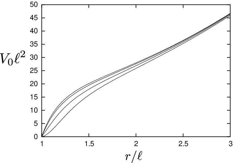
We consider the stability of this mode. In this mode, the master equation (B.5) is in the Schrödinger form. Therefore, positivity of means stability of this mode. The typical profile of is shown in Figure. 5. We can see the positivity of this potential from this figure. In fact, the positivity can be checked from the expression (B.7). From Eq. (2.9) and (2.10), we obtain
| (B.8) |
The right hand side is an increasing function of which approaches to in the limit of . Thus, we can get the inequality . Therefore, negative terms in the big brackets of Eq. (B.7) are and terms. To see positivity of , we focus on , and terms in the big bracket of Eq. (B.7). After dividing them by , these terms become
| (B.9) |
If is positive, is also positive. Now, we substitute Eq. (2.10) into Eq. (B.9). Because of and , we can put for and . Then, we can obtain
| (B.10) |
where , and . We can see explicitly. It means the stability of mode.
B.2 with mode
In mode, there are fields. We set as
| (B.11) |
With the gauge parameter , the gauge transformations for these components are given by
| (B.12) |
Our gauge choice is
| (B.13) |
This condition fixes the gauge completely. After the gauge fixing, two fields and are remained. However, because one constraint exists in this mode, the physical degree of freedom becomes one. Therefore, we can get one master equation. Substituting Eq. (B.11) and Eq. (B.13) into Eq. (3.2), we can get the master equation for this mode,
| (B.14) |
where we have defined a new variable,77 7 This choice of master variable is important. If we use other master variable, the terms may appear in the resultant master equation. The good master variable (B.15) can be found by moving into the Hamiltonian formalism as explained in [21].
| (B.15) |
and functions and are given by
| (B.16) |
and
| (B.17) |
We have used the tortoise coordinate defined in Eq. (3.17).
We can get the asymptotic form of and as
| (B.18) |
and
| (B.19) |
Therefore, asymptotic form of solution of master equation (B.14) becomes
| (B.20) |
We can study the onset of superradiant instability of this mode by the same way as section 3.3. The result is depicted in Figure.6. We see that onset of the instability is . On the other hand, in section 3.3, it was shown that the onset is for modes. Thus, the mode is irrelevant for the onset of the instability.

B.3 with modes
To see the effect of Kaluza-Klein modes for superradiant instability, we study the stability of with modes. The metric perturbation for these mode is given by
| (B.21) |
where and is spherical harmonics on defined by (4.2). We define a new variable as
| (B.22) |
Then, using (4.3), we can obtain equation for these modes as
| (B.23) |
where functions and are determined by
| (B.24) |
and
| (B.25) |
The equations (B.23) return to (3.15) for . By the similar way as section 3.3.2, we can see that, for small black holes, the onset of superradiant instability is given by . For any value of , we solve (B.23) numerically by the same way as section 3.3.3 and obtain Figure.7. We plot the onset of instability for and modes. From this result, we can see that the superradiant instability of Kaluza-Klein modes appear at higher than zero mode. Thus, this result suggest that Kaluza-Klein modes are not relevant to see the onset of superradiant instability.

Appendix C Transverse Traceless Condition for Kaluza-Klein Graviton
In this appendix, we prove that we can impose the transverse traceless condition (4.5) in the equation (4.3).
From the Bianchi identity, we can get
| (C.1) |
where is perturbation of the Christoffel symbol defined by
| (C.2) |
The back ground equation is given by and, thus, we can get . Therefore, the first term in the second line of (C.1) vanishes and we can get
| (C.3) |
where we have used the expression (C.2) at the last equality. Hence, from the divergence of the perturbation equation (4.3),
| (C.4) |
It is the constraint equation of (4.3).
Now, we consider the trace of (4.3). The trace of perturbation of the Einstein tensor is given by
| (C.5) |
Because of and , Ricci tensor and Ricci scalar terms in (C.5) are cancelled each other. Thus, making use of the constraint equation (C.4), the equation (C.5) becomes
| (C.6) |
Thus, from the trace of (4.3), we can get the equation for trace part of as
| (C.7) |
Therefore, trace part of is decoupled from other components of and we can put consistently. Then, constraint equation becomes .
References
- [1] J. M. Maldacena, “The large N limit of superconformal field theories and supergravity,” Adv. Theor. Math. Phys. 2, 231 (1998) [Int. J. Theor. Phys. 38, 1113 (1999)] [arXiv:hep-th/9711200].
- [2] S. S. Gubser, I. R. Klebanov and A. M. Polyakov, “Gauge theory correlators from non-critical string theory,” Phys. Lett. B 428, 105 (1998) [arXiv:hep-th/9802109].
- [3] E. Witten, “Anti-de Sitter space and holography,” Adv. Theor. Math. Phys. 2, 253 (1998) [arXiv:hep-th/9802150].
- [4] O. Aharony, S. S. Gubser, J. M. Maldacena, H. Ooguri and Y. Oz, “Large N field theories, string theory and gravity,” Phys. Rept. 323, 183 (2000) [arXiv:hep-th/9905111].
- [5] H. Kodama and A. Ishibashi, “A master equation for gravitational perturbations of maximally symmetric black holes in higher dimensions,” Prog. Theor. Phys. 110, 701 (2003) [arXiv:hep-th/0305147].
- [6] A. Ishibashi and H. Kodama, “Stability of higher-dimensional Schwarzschild black holes,” Prog. Theor. Phys. 110, 901 (2003) [arXiv:hep-th/0305185].
- [7] H. Kodama and A. Ishibashi, “Master equations for perturbations of generalized static black holes with charge in higher dimensions,” Prog. Theor. Phys. 111, 29 (2004) [arXiv:hep-th/0308128].
- [8] R. A. Konoplya and A. Zhidenko, “Stability of higher dimensional Reissner-Nordstrom-anti-de Sitter black holes,” arXiv:0809.2048 [hep-th].
- [9] R. A. Konoplya and A. Zhidenko, “Stability of multidimensional black holes: Complete numerical analysis,” Nucl. Phys. B 777, 182 (2007) [arXiv:hep-th/0703231].
- [10] V. Cardoso and O. J. C. Dias, “Small Kerr-anti-de Sitter black holes are unstable,” Phys. Rev. D 70, 084011 (2004) [arXiv:hep-th/0405006].
- [11] V. Cardoso, O. J. C. Dias and S. Yoshida, “Classical instability of Kerr-AdS black holes and the issue of final state,” Phys. Rev. D 74, 044008 (2006) [arXiv:hep-th/0607162].
- [12] V. Cardoso, R. Konoplya and J. P. S. Lemos, “Quasinormal frequencies of Schwarzschild black holes in anti-de Sitter spacetimes: A complete study on the asymptotic behavior,” Phys. Rev. D 68, 044024 (2003) [arXiv:gr-qc/0305037].
- [13] H. K. Kunduri, J. Lucietti and H. S. Reall, “Gravitational perturbations of higher dimensional rotating black holes: Tensor Perturbations,” Phys. Rev. D 74, 084021 (2006) [arXiv:hep-th/0606076].
- [14] H. Kodama, “Superradiance and Instability of Black Holes,” Prog. Theor. Phys. Suppl. 172, 11 (2008) [arXiv:0711.4184 [hep-th]].
- [15] H. Kodama, R. A. Konoplya and A. Zhidenko, “Gravitational instability of simply rotating Myers-Perry-AdS black holes,” arXiv:0812.0445 [hep-th].
- [16] B. M. N. Carter and I. P. Neupane, “Thermodynamics and stability of higher dimensional rotating (Kerr) AdS black holes,” Phys. Rev. D 72, 043534 (2005) [arXiv:gr-qc/0506103].
- [17] A. N. Aliev and O. Delice, “Superradiant Instability of Five-Dimensional Rotating Charged AdS Black Holes,” arXiv:0808.0280 [hep-th].
- [18] K. Murata and J. Soda, “A Note on Separability of Field Equations in Myers-Perry Spacetimes,” Class. Quant. Grav. 25, 035006 (2008) [arXiv:0710.0221 [hep-th]].
- [19] M. Kimura, K. Murata, H. Ishihara and J. Soda, “On the Stability of Squashed Kaluza-Klein Black Holes,” Phys. Rev. D 77, 064015 (2008) [arXiv:0712.4202 [hep-th]].
- [20] H. Ishihara, M. Kimura, R. A. Konoplya, K. Murata, J. Soda and A. Zhidenko, “Evolution of perturbations of squashed Kaluza-Klein black holes: escape from instability,” Phys. Rev. D 77, 084019 (2008) [arXiv:0802.0655 [hep-th]].
- [21] K. Murata and J. Soda, “Stability of Five-dimensional Myers-Perry Black Holes with Equal Angular Momenta,” arXiv:0803.1371 [hep-th].
- [22] R. Gregory and R. Laflamme, “Black strings and p-branes are unstable,” Phys. Rev. Lett. 70, 2837 (1993) [arXiv:hep-th/9301052].
- [23] R. Gregory and R. Laflamme, “The Instability of charged black strings and p-branes,” Nucl. Phys. B 428, 399 (1994) [arXiv:hep-th/9404071].
- [24] T. Harmark, V. Niarchos and N. A. Obers, “Instabilities of black strings and branes,” Class. Quant. Grav. 24, R1 (2007) [arXiv:hep-th/0701022].
- [25] V. E. Hubeny and M. Rangamani, “Unstable horizons,” JHEP 0205, 027 (2002) [arXiv:hep-th/0202189].
- [26] S. W. Hawking, C. J. Hunter and M. Taylor, “Rotation and the AdS/CFT correspondence,” Phys. Rev. D 59, 064005 (1999) [arXiv:hep-th/9811056].
- [27] G. W. Gibbons, H. Lu, D. N. Page and C. N. Pope, “Rotating black holes in higher dimensions with a cosmological constant,” Phys. Rev. Lett. 93, 171102 (2004) [arXiv:hep-th/0409155].
- [28] G. W. Gibbons, H. Lu, D. N. Page and C. N. Pope, “The general Kerr-de Sitter metrics in all dimensions,” J. Geom. Phys. 53, 49 (2005) [arXiv:hep-th/0404008].
- [29] G. W. Gibbons, M. J. Perry and C. N. Pope, “The first law of thermodynamics for Kerr - anti-de Sitter black holes,” Class. Quant. Grav. 22, 1503 (2005) [arXiv:hep-th/0408217].
- [30] B. L. Hu, “Separation of tensor equations in a homogeneous space by group theoretical methods,” J. Math. Phys. 15, 1748 (1974).
- [31] W. H. Press, S. A. Teukolsky, Astrophys. J. 185, 649 (1973)
- [32] R. A. Konoplya, “On quasinormal modes of small Schwarzschild-anti-de-Sitter black hole,” Phys. Rev. D 66, 044009 (2002) [arXiv:hep-th/0205142].
- [33] S. W. Hawking and H. S. Reall, “Charged and rotating AdS black holes and their CFT duals,” Phys. Rev. D 61, 024014 (2000) [arXiv:hep-th/9908109].
- [34] K. Murata, T. Nishioka, N. Tanahashi and H. Yumisaki, “Phase Transitions of Charged Kerr-AdS Black Holes from Large-N Gauge Theories,” arXiv:0806.2314 [hep-th].
- [35] O. Aharony, J. Marsano, S. Minwalla and T. Wiseman, “Black hole - black string phase transitions in thermal 1+1 dimensional supersymmetric Yang-Mills theory on a circle,” Class. Quant. Grav. 21, 5169 (2004) [arXiv:hep-th/0406210].
- [36] T. Harmark and N. A. Obers, “New phases of near-extremal branes on a circle,” JHEP 0409, 022 (2004) [arXiv:hep-th/0407094].
- [37] M. Hanada and T. Nishioka, “Cascade of Gregory-Laflamme Transitions and U(1) Breakdown in Super Yang-Mills,” JHEP 0709, 012 (2007) [arXiv:0706.0188 [hep-th]].
- [38] T. Hollowood, S. P. Kumar and A. Naqvi, “Instabilities of the small black hole: A view from N = 4 SYM,” JHEP 0701, 001 (2007) [arXiv:hep-th/0607111].
- [39] M. Cvetic and S. S. Gubser, “Phases of R-charged black holes, spinning branes and strongly coupled gauge theories,” JHEP 9904, 024 (1999) [arXiv:hep-th/9902195].
- [40] D. Yamada and L. G. Yaffe, “Phase diagram of N = 4 super-Yang-Mills theory with R-symmetry chemical potentials,” JHEP 0609, 027 (2006) [arXiv:hep-th/0602074].
- [41] R. Emparan and H. S. Reall, “A rotating black ring in five dimensions,” Phys. Rev. Lett. 88, 101101 (2002) [arXiv:hep-th/0110260].
- [42] M. M. Caldarelli, R. Emparan and M. J. Rodriguez, “Black Rings in (Anti)-deSitter space,” JHEP 0811, 011 (2008) [arXiv:0806.1954 [hep-th]].
- [43] P. Bizon, T. Chmaj, G. W. Gibbons and C. N. Pope, “Gravitational solitons and the squashed seven-sphere,” Class. Quant. Grav. 24, 4751 (2007) [arXiv:hep-th/0701190].