Generalised Kramers model
Abstract
We study a particular generalisation of the classical Kramers model describing Brownian particles in the external potential. The generalised model includes the stochastic force which is modelled as an additive random noise that depends upon the position of the particle, as well as time. The stationary solution of the Fokker-Planck equation is analysed in two limits: weak external forcing, where the solution is equivalent to the increase of the potential compared to the classical model, and strong external forcing, where the solution yields a non-zero probability flux for the motion in a periodic potential with a broken reflection symmetry.
pacs
05.40.-a, 05.60.Cd, 05.10.GgI Introduction
This paper addresses the problem of the overdamped motion of independent particles in the external potential subjected to a random forcing in one spatial dimension. The model is an extension of the so-called Kramers model [1] in which a particle at the position executes creeping motion according to the following equation of motion:
| (1) |
Here, is the friction coefficient, is the potential, and is the stochastic force which is usually modelled as a rapidly fluctuating time-dependent random noise. We generalise this model by considering the random force which depends not only upon time, but also upon the position of the particle. This generalisation is proposed in the same way as the one discussed for a closely related model of inertial particles (the Ornstein-Uhlenbeck process [2]) studied earlier by the author of this paper in collaboration (see [3, 4]). Such a generalisation of the Ornstein-Uhlenbeck process leads to a number of non-trivial results: non-Maxwellian stationary distribution of the velocity, anomalous diffusion of the velocity and position, and ‘staggered ladder’ spectra of the corresponding Fokker-Planck operator.
The model of Brownian particles in the external potential has a large number of important applications in physics and chemistry and below we briefly discuss two of them. First example is a model of chemical reaction processes, where the position of the particle represents the reaction coordinate which undergoes a noise-activated escape process driven by thermal fluctuations [5]. The reaction coordinate is a rather abstract notion in chemistry characterising the state of a chemical reaction. Typically, the coordinate wiggles around one of the minima of the potential energy profile, until a sequence of random ‘kicks’ induced by thermal fluctuations transports it over the potential barrier, so that its dynamics can be accurately described by the motion of the Brownian particle in the external potential.
The other interesting application of the Kramers model concerns a concept of the Brownian ratchet, which was originally introduced by Feynman [6] to illustrate laws of thermodynamics. In its simplest form, the device consists of a ratchet, which resembles a circular saw with asymmetric teeth, rotating freely in one particular (forward) direction. A pawl is attached to the ratchet, thus preventing it to rotate in the other (backward) direction. The ratchet is connected to a paddle wheel by a massless frictionless rod and the whole mechanism is immersed in a thermal bath at a given temperature. It is assumed that the mechanism is so small that the paddle wheel can rotate in response to collisions with the molecules of the thermal bath, thus rotating back and forth. Because the pawl restricts the backward rotation, the ratchet slowly spins forward as the molecules hit the paddle-wheel. If a weight is attached to the rod connecting the ratchet and the paddle wheel, it would be lifted by this forward rotation making the device ‘perpetuum mobile’ of the second kind. The contradiction is resolved by noting that the device must be very small in order to react to individual collisions with the molecules. This means that the pawl itself must be influenced by the collisions, so that every now and then it would be lifted and fail to prevent the backward rotation. Since both the paddle wheel and the ratchet are immersed in the same thermal bath, the probability for the pawl to fail is the same as the probability for the ratchet to rotate forward, so that no net work can be extracted. The analogy with the model of the Brownian particle in the potential is evident. If the position of the particle represents the angle of rotation of the rod, then the dynamics is periodic and can be split up into two parts: random fluctuations induced by collisions of the paddle wheel with the molecules and motion in the potential representing the interaction between the pawl and teeth of the ratchet. The potential in this case is periodic and asymmetric (the so-called ‘sawtooth’ potential). The analysis of the classical model shows that there is no net transport (probability flux) of the Brownian particles moving in a periodic and asymmetric potential.
In many problems it suffices to know the probability density function (PDF) of the position of the particle in the steady state in order to understand all important properties of the Kramers model. The principal result of this paper is the PDF of the position of the particle in the generalised model in the limit of short correlation time of the random force.
We proceed as follows. We start by describing the generalised model and introducing properties of the stochastic force. In the limit of short correlation time of the stochastic force the PDF satisfies the Fokker-Planck equation, which we derive for the general case. The stationary solution of the Fokker-Planck equation can be simplified in two asymptotic limits, corresponding to very large and very small values of the external potential force. The generalised model in the weak external force limit was first considered in [7], where the PDF was found to be equivalent to a reduction of the potential compared with the classical Kramers model. Here, a more transparent analysis is used giving rise to many additional results. We find that in the weak forcing limit the generalisation leads to an effective increase of the potential, rather than a decrease derived in [7]. In the strong forcing limit we find the solution that corresponds to a non-zero probability flux in the case of the motion in a periodic potential with a broken reflection symmetry.
II Stochastic model
Let us consider a very small particle moving in the potential and subject to the stochastic force in one spatial dimension. For a particle with a negligible mass the velocity is determined by the balance of the forces acting upon it, so that the equation of motion reads
| (2) |
where is the external potential force. The random force in (2) is assumed to be a stationary and translationally invariant Gaussian process with zero mean and correlation function
| (3) |
where angular brackets denote average over noise realisations throughout. The noise has a typical magnitude , correlation length , and correlation time . We assume that the correlation function is smooth and sufficiently differentiable and decays rapidly for and . In the absence of the external potential the particle is not bounded and diffuses, so that the mean square displacement is given by with a diffusion constant for . Relaxation towards a statistically stationary state is associated with the action of the potential. The corresponding relaxation time depends upon particular properties of the potential, as well as properties of the random force, but in the general case it cannot be determined explicitly.
III Fokker-Planck equation
If the correlation time of the random force is sufficiently short (that is ), it is possible to define a time scale at which the stochastic force fluctuates appreciably, while the change of the dynamical variable is negligible on the length scale of the potential, . Integrating the equation of motion (2) over the time period we obtain
| (4) |
Following the standard procedure (see, e.g. [8]), we write the Fokker-Planck equation for the probability density function for the stochastic model given by Eq. (2) in the limit of short correlation time of the random force:
| (5) |
Here, is the drift velocity and is the diffusion coefficient defined via the increment as follows:
| (6) |
In the following sections we use stationary and translationally invariant properties of the noise and set and in Eq. (4) for calculating statistical properties of . Using Eq. (4) we obtain
| (7) |
We are interested in the stationary solution of Eq. (5) satisfying . It is found by solving the differential equation
| (8) |
where the stationary probability flux is determined from the boundary conditions. The solution of Eq. (8) can be readily written as
| (9) |
where
| (10) |
and is the normalisation constant. We remark that in the case of a periodic potential is normalised in the periodicity interval. The rest of the paper is concerned with simplifying the solution (9) in two asymptotic limits corresponding to very large and very small values of the external force .
It is not typical to have a non-zero flux in systems that are in thermal equilibrium. The cases where the transport can be introduced by different mechanisms are of great interest. Feynman considered the case where the ratchet and the paddle-wheel are immersed in separate thermal baths at different temperatures. In this case, the transport is induced by the gradient of the temperature. The transport in the Kramers model may also be induced by an addition of another driving force that can be constant [9] or a function of time [10]. We also remark that the Fokker-Planck equation with the state-dependent diffusion coefficient was studied before in [11, 12], where the transport in a symmetric periodic potential is a consequence of the non-uniform intensity of the stochastic force modelled as a multiplicative noise, i.e. , where is periodic and is a rapidly fluctuating random noise. In this paper we show that it is possible to obtain a non-zero flux even for a model where the noise is additive and has translationally invariant statistics.
We conclude this section by discussing conditions and limits of validity of the Fokker-Planck equation for our model. The question of the validity of the Fokker-Planck approach is rather hard to discuss in precise terms for the problems which involve spatial dependence of the additive noise. The important quantity in this case is the effective correlation time of the stochastic force, i.e. how rapidly the force experienced by the moving particle de-correlates. It is evident that the additional correlation in space may only decrease this effective correlation time. The Fokker-Planck approach relies mainly on two conditions: short correlation time of the stochastic force and small change of the dynamical variable in . The first condition has already been mentioned earlier and reads , where is the relaxation time. As for the small increment, the obvious condition would be . Again, this condition is only approximate, since the effective correlation time is not known explicitly.
IV Weak external force limit
Let us consider the increment in the limit when the motion of the particle is dominated by the stochastic force. First, we introduce some additional notation:
| (11) |
Using this we can write the increment from Eq. (4) as follows:
| (12) |
Expanding in the series the stochastic force about we obtain
| (13) |
Averaging this expression we obtain
| (14) |
We now simplify the problem by considering the case when the spatial dependence of the random force is weak or, equivalently, when the correlation length is sufficiently large. Let us introduce a quantity which measures a distance travelled by the particle due to the random force in the correlation time relative to the correlation length:
| (15) |
We term this parameter the Kubo number. It has been used before in the similar context of motion of inertial particles (see e.g. [13]). We remark that the classical Kramers model corresponds to . When the Kubo number is small, we can write the firs moment of by expanding the stochastic force further:
| (16) | |||||
From the properties of the random force we have and , and using the definition of we obtain
| (17) | |||||
Next, we expand . We note that for any and , and after dropping terms of order higher than we obtain
| (18) | |||||
For the two-point correlation function in this expression we use the following identities which hold for any stationary Gaussian noise:
| (19) |
Using this we obtain
| (20) | |||||
The integrand in the last term depends only upon and is therefore linear in . In the remaining part of the paper we shall deal with similar double and quadruple integrals, so now we discuss the last term in more details. Let us consider a double integral
| (21) |
We denote and obtain
| (22) |
In Fig. 1 we illustrate this transformation of variables. For the integrand is significant around and decreases rapidly for increasing. Thus, if we integrate for from to , we would only make a small error of order . Using this we may write
| (23) |
Assuming that the last integral is convergent we obtain
| (24) |

We return to the calculation of and obtain
| (25) |
The drift velocity then reads
| (26) |
where
| (27) |
The sign of can be deduced as follows. If we can write the correlation function in the form , where , then the sign of is determined by the sign of . If the random force de-correlates as increases, then is a local maximum of . Providing that the second derivative exists, it follows that and, consequently, . Furthermore, we have , and therefore . We remark that if we keep expanding the stochastic force further in Eq. (17), we would obtain terms of order higher than .
We now calculate and the diffusion coefficient. After squaring and averaging Eq. (13) we obtain
| (28) | |||||
The second term on the right hand side in this expression is at least . This becomes obvious if we notice that the correlation function in the integrand depends on , but due to the factor the whole integrand cannot be expressed as a function of only. The diffusion coefficient is therefore given by
| (29) |
If we proceed to expand the stochastic force further, we would obtain terms which are at least . We therefore conclude that the diffusion coefficient in this case is constant and is the same as in the model of free diffusion given by the equation
| (30) |
Let us now consider a case of small Kubo number similarly to the calculation of the drift velocity. We shall consider this case as a separate problem and discuss it in the appendix. We obtain that in the limit of small (or small ) the diffusion constant is given by
| (31) |
where is the diffusion constant for the model in the absence of the spatial correlation corresponding to . It is given by
| (32) |
The factor is given by
| (33) |
Thus, the diffusion constant is reduced by the factor compared to the case of . Using Eqs. (26) and (31) we obtain the solution of the Fokker-Planck equation in the weak forcing limit corresponding to small :
| (34) |
where
| (35) |
We now concentrate on the form of the solution (34) for particular choices of the potential illustrated in Fig. 2. First example is a symmetric double-well potential used in modelling two-way chemical reactions, and the other is a periodic potential with period . For the double-well potential illustrated in Fig. 2a the natural boundary conditions are applied [14]:
| (36) |
Such a potential does not allow the particles to escape to infinity, so that we expect that the probability flux vanishes. We note that goes to zero for very large and the second term in the brackets multiplied by approaches a non-zero constant. Thus, the boundary conditions are satisfied only when .

For the periodic potential, if we require that is bounded for the increasing , it follows that is periodic [14]. We use to obtain and therefore the condition of periodicity reads
| (37) |
The integral in the last term is non-zero, therefore we again put to satisfy the boundary conditions. The important consequence of this result is that the flux vanishes regardless of the shape of the periodic potential. In the studies of Brownian ratchets it is often assumed that the periodic potential has an asymmetric form (such as the ‘sawtooth’ potential illustrated in Fig. 2c), so that the particles are expected to favour the slope with a smaller inclination to escape the potential minimum. The result shows, however, that the probability flux vanishes, which agrees with the discussion of the Brownian ratchet in the introduction.
We conclude that in both examples the solution in the weak external force limit is given by
| (38) |
This is the Maxwellian density with the potential increased by the factor compared with the classical Kramers model, which corresponds to . The solution is consistent with the idea that in the presence of spatial correlations the noise experienced by the moving particle de-correlates more rapidly than for the case of an infinite correlation length in the classical Kramers model. This means that the particle experiences more uncorrelated kicks along its trajectory decreasing the probability to travel far against the systematic force . Therefore, we expect to see the density function becoming sharper around the minima of the potential as the correlation length decreases. Our result differs from the one obtained in [7], where the effective decrease of the potential in the solution is attributed to the reduction of the drift velocity given by Eq. (26), but the corresponding reduction of the diffusion coefficient is not considered.
We remark that in the general case, when the potential force is weak, the drift reduction remains linear in and the diffusion coefficient remains constant, even when is not small. The actual values of and in the case of arbitrary Kubo number are not known, but the density still remains Maxwellian around stagnation points of the potential, provided that the Fokker-Planck approach remains valid.
V Strong external force limit
In this section we analyse the limit when the motion of the particle is dominated by the external potential force. In this case we can expand the stochastic force in the series about . The increment in this case reads
| (39) |
We first calculate . The term is obviously of order and so is the mixed product of and the integral terms in the expression above. The rest of the terms require some careful considerations. We have
| (40) | |||||
For the first term we obtain
| (41) | |||||
The integrand in the last expression depends only on and is therefore of order when . Similarly to the cases considered in the previous section (see Eq. (21)) we obtain
| (42) |
We now proceed a step further and calculate this term expanding for large . Using the definition of in Eq. (11) we can write this by changing the variable from to
| (43) | |||||
The modulus sign is used to ensure that the expression remains positive. Thus, in the limit of strong external forcing the first term in is inversely proportional to . Now we return to the starting point (Eq. (40)) and consider for instance the term
| (44) | |||||
The four-point correlation function for a Gaussian random process can be expressed as the sum of all possible non-repeating combinations of products of two-point correlation functions. A typical combination in this case may look as follows:
| (45) | |||||
If we proceed in the same way as for the previous term expanding for large , each of the factors would contribute at least , so that the overall contribution would be of order , and therefore may be neglected. Similarly, the remaining term in Eq. (40) may also be neglected. We conclude that the diffusion coefficient is determined by Eq. (43) and reads
| (46) |
We rewrite this as follows:
| (47) |
We now consider :
| (48) |
Here, the second term vanishes because effectively the average is taken over a deterministic trajectory, since the potential is assumed to be varying slowly. For the second term we obtain
| (49) |
neglecting terms of higher orders in . We then obtain
| (50) |
If we proceed further and expand this expression for strong external force, we obtain the term which is inverse proportional to , similarly to the calculation of . Since , we therefore conclude that the first moment of in the limit of strong external force reads
| (51) |
The drift velocity is therefore given by
| (52) |
Substituting (47) and (52) into (9) we obtain the solution in the strong external force limit:
| (53) |
where
| (54) |
For the non-periodic potential, if we can again show that . We note that diverges for large , whereas the integral term in the brackets multiplied by converges to a constant for large . The solution corresponding to is given by
| (55) |
For the case of a periodic potential with the period we find by writing as
| (56) |
Using we obtain
| (57) |
We note that for the periodic potential and thus the solution in the strong external force limit can be written in the following compact form:
| (58) |
For the periodic potential we have obtained a peculiar result: if the solution of the Fokker-Planck equation corresponds to a non-zero probability flux in the stationary state. For any periodic potential integrating in the periodicity interval gives 0. Thus, if the expression for contained only , the flux would vanish. Because the integrand in Eq. (54) is quadratic in , the sign of is determined by the sign of the steepest of two slopes of the potential, if we consider a case of the potential with a single minimum in the periodicity interval. Thus, if the periodic potential is symmetric (such as the one in Fig. 2b), then and vanishes. Conversely, for a ‘sawtooth’ potential with a broken reflection symmetry (Fig. 2c), and the solution of the Fokker-Planck equation corresponds to a non-zero probability flux.
VI Numerical simulations and discussion
We perform a number of numerical experiments in order to illustrate our analytical results. Numerical simulations are done by integrating the original equation of motion (2) using a small time step (typically about ). In the simulations we use the following correlation function of the random force:
| (59) |
We use two different types of the potential corresponding to the examples given in sections IV and V: an asymmetric periodic potential and a non-periodic double-well potential . The relaxation time is of order unity in all simulations (as judged from the plot versus ), so that the Fokker-Planck approach is valid for the values of typically smaller than .
VI.1 Free diffusion
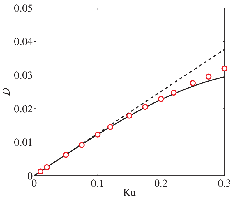
We start by illustrating the reduction of the diffusion constant in the model of free diffusion () in the limit of small Kubo number. For the correlation function given by Eq. (59) we obtain
| (60) |
The diffusion constant is reduced according to Eq. (31):
| (61) |
In Fig. 3 we show the results of the numerical simulations and compare them with our analytical result. The agreement with Eq. (31) remains very accurate up to values of around 0.25. For larger Kubo number it is required to take into account terms of higher order in the expansion discussed in the appendix (Eq. (66)). As an example, we also calculate the diffusion constant for the correlation function :
| (62) |
VI.2 Results for the weak external force limit


We continue by illustrating the results in the presence of the potential in the limit of small . The numerical results and their comparison with the theory in this case are presented in Fig. 4. For the double-well potential the particles are concentrated around two minima of the potential with a spread which is smaller compared to the classical Kramers model, where the correlation length is infinite. When the Kubo number is small, the particles almost always stays in the region of small for the double-well potential, so that the PDF is Maxwellian and accurately given by Eq. (38). For the periodic potential the value of the external force is bounded by the value of , which is kept sufficiently small. Although the difference between the results for the classical Kramers model and the generalised one is quite marginal for small , the tendency of the effective increase of the potential is evident.
VI.3 Results for the strong external force limit
Finally, we comment on the results for the strong external force limit, summarised in Fig. 5. We remark that the probability for the particle to propagate to the regions where is large is typically very small. Thus, we expect our theoretical result to give a good agreement with the tails of the PDF far from the stagnation points of the potential. This agreement is best seen on the logarithmic scale, as shown in Figs. 5e and 5f. Around the stagnation points of the potential we approximate the PDF by the Maxwellian distribution and choose to give the best agreement with the data from the simulations.
The case of an asymmetric periodic potential is particularly interesting, since it exhibits a non-zero probability flux. As we have already discussed in section V, if the potential is asymmetric, the particles are expected to favour a slope with a smaller inclination to escape the minimum. The direction of the transport in the generalised model can be deduced from Eq. (54). We note that the sign of is determined by the sign of the steepest of two slopes of the potential. In Fig. 5, it is the slope to the right of the minimum that corresponds to and . From Eq. (57) we obtain , implying that it is easier for particles to escape from the minimum using a left slope, as expected.
References
- [1] H. A. Kramers, Physica (Utrecht), 7, 284 (1940).
- [2] G. E. Ornstein and L. S. Uhlenbeck, Phys. Rev., 36, 823 (1930).
- [3] E. Arvedson, B. Mehlig, M. Wilkinson, and K. Nakamura, Phys. Rev. Lett., 96, 030601 (2005).
- [4] V. Bezuglyy, B. Mehlig, M. Wilkinson, K. Nakamura, and E. Arvedson, J. Math. Phys., 47, 073301 (2006).
- [5] P. Hänggi, P. Talkner, and M. Borkovec, Rev. Mod. Phys., 62, 251 (1990).
- [6] R. P. Feynman, R. B. Leighton, and M. Sands, The Feynman Lectures on Physics, vol. 1, Addison-Wesley, Reading, MA (1966).
- [7] T. Monnai, A. Sugita, and K. Nakamura, Europhys. Lett., 84, 20005 (2008).
- [8] N. G. van Kampen, Stochastic processes in physics and chemistry, 2nd ed., North-Holland, Amsterdam (1981).
- [9] P. Reimann, Phys. Rep., 361, 57 (2002).
- [10] M. O. Magnasco, Phys. Rev. Lett., 71, 1477 (1993).
- [11] M. Büttiker, Z. Phys. B, 68, 161 (1987).
- [12] N.G. van Kampen, IBM J. Res. Develop., 32, 107 (1988).
- [13] K. Duncan, B. Mehlig, S. Östlund, and M. Wilkinson, Phys. Rev. Lett., 95, 240602 (2005).
- [14] H. Risken, The Fokker-Planck Equation. Methods of Solutions and Applications, Springer, New York (1999).
Appendix A Diffusion constant in the limit of small Kubo number
In the appendix we discuss the problem of free diffusion in the limit of small Kubo number. We consider a particle at the position moving with the random velocity , so that the equation of motion reads
| (63) |
The random velocity is a stationary and translationally invariant Gaussian random process with zero mean and correlation function . We denote the typical magnitude of the velocity by and the correlation time and correlation length by and , respectively. The correlation function is assumed to be smooth and differentiable and decays rapidly for and . The Kubo number measures a typical distance travelled by the particle in one correlation time relative to the correlation length:
| (64) |
Assuming that the displacement after time is
| (65) |
In the limit of small the spatial dependence of the random velocity is weak, so that we can expand the trajectory in the series as follows:
| (66) |
This expansion includes all the terms which will yield only two- and four-point correlation functions. After squaring and averaging Eq. (66) we obtain
| (67) | |||||
Expanding and further we obtain
| (68) | |||||
Here, the first term corresponds to the motion of the particle in the absence of spatial dependence of the velocity. Assuming that we obtain
| (69) |
where
| (70) |
For the rest of the terms in Eq. (68) we use the following statistical properties of a Gaussian noise:
| (71) |
In the discussion below we shall drop the spatial argument of the correlation function implying that . We have
| (72) | |||||
We note that the following relation holds for any and the correlation function which can be written in the form :
| (73) |
Using this we can combine the terms in Eq. (72) together and obtain
| (74) | |||||
We now calculate the remaining two terms. We first consider
| (75) |
We put and to obtain
| (76) |
We note that is significant around for . We have
| (77) |
Now, we denote and obtain
| (78) |
or
| (79) |
where
| (80) |
We remark that or, equivalently, .
We now consider the third term in Eq. (74):
| (81) |
We introduce new variables and and obtain
| (82) |
The integrand here is significant around , so that we can write
| (83) |
We denote and obtain
| (84) |
For we have
| (85) |
or
| (86) |
where
| (87) |
We note that the integrand is significant around so that we can write
| (88) |
and therefore
| (89) |
where is defined similarly to Eq. (27):
| (90) |
We remark that . Going back to Eq. (74) we obtain
| (91) |
We may define the effective diffusion constant , so that the mean square displacement can be written as
| (92) |
In the view that , we may write for some factor which can be expressed from Eq. (80). The effective diffusion constant is then given by
| (93) |
We remark that both and are negative for and . Thus, the diffusion constant is reduced and the reduction is proportional to when is small.