Time reversal in thermoacoustic tomography - an error estimate

Thermoacoustic tomography is a hybrid medical imaging technique characterized by high resolution and contrast. A short electromagnetic pulse is used to irradiate the biological object of interest. A part of the electromagnetic energy is absorbed by the tissue, which causes a thermoelastic expansion. This leads to a pressure wave propagating through the object, which is measured by ultrasound transducers located on an observation surface $S$, usually surrounding the object. The collected information is used to reconstruct the initial pressure, which is roughly proportional to the absorbed energy [1, 2]. The good contrast in the resulting images is due to electromagnetic energy being preferentially absorbed by cancerous cells, while ultrasound provides a submilimeter resolution [3, 2].

Let $S$ be a smooth observation surface surrounding the object and let $B$ be the domain bounded by $S$. In applications only space dimensions $n=2,3$ are of interest, but the analysis developed in this paper is carried out for an arbitrary dimension $n$. We assume that the speed $c(x)$ of ultrasound in the tissue is smooth and strictly positive $c(x)>c>0$, and that $c(x)\equiv 1$ for large values of $|x|$. Then the pressure $p(x,t)$ at location $x$ and time $t$ satisfies the wave equation (e.g. [4, 5, 1, 6]):

$$\left\{\begin{array}[]{cc}p_{tt}=c^{2}(x)\Delta p,&t\geq 0,\quad x\in\mathbb{R}^{n}\\ p(x,0)=f(x),&p_{t}(x,0)=0,\\ p(y,t)=g(y,t)&\mbox{ for }y\in S,\quad t\geq 0.\end{array}\right.$$

(1)

Here $p_{tt}$ denotes the second time derivative of $p(x,t)$, $g(y,t)$ is the measured data, i.e. the value of the pressure at time $t$ measured at transducer’s location $y\in S$, and $f(x)$ is the initial pressure, which is to be reconstructed. The function $f(x)$ is assumed to have a compact support in $B$. One thus faces the problem of inverting the mapping $R\colon f\rightarrow g$ from the initial pressure to the measured data. For a more detailed description of the mathematical methods used in thermoacoustic tomography, one can refer to [7, 6, 8, 9, 10, 11] and the references therein. There are various types of reconstruction procedures for closed observation surfaces, e.g. filtered backprojection formulas, eigenfunction expansion methods and time reversal method. A comparison of the three and a discussion of their advantages and limitations can be found in [12]. It was argued there that time reversal is the most versatile and easy to implement among these. Here we consider the errors involved in the time reversal method and provide estimates that justify its validity. It should be noted that, although we are interested in applications to thermoacoustic tomography, the time reversal method for the wave equation has been used in other applications [13, 14, 15]. Our results apply in all these cases.

In Section 2 a non-trapping condition on the sound speed is recalled and the time reversal method is described. In Section 3 the main result of this artice is formulated and proved. Numerical examples are provided in Section 4. Section 5 contains some concluding remarks. This is followed by the acknowledgment section.

Additional discussions and implementations of the time reversal method can be found in [16, 17, 12].

In this section we give a more detailed description of the time reversal method and recall the notion of a non-trapping sound speed.

Consider the error $e(x,t;T)=u(x,t)-v(x,t)$ that results from replacing the true solution of (5), $u(x,t)$, with the time reversal solution $v(x,t)$. Recall that $v(x,t)$ solves equation (6). Then, the error satisfies the following equation:

$$\left\{\begin{array}[]{l}e_{tt}(x,t;T)=c^{2}(x)\Delta e(x,t;T)\qquad\mbox{in}\;B\times[0,T]\\ e(x,T;T)=p(x,T)\\ e_{t}(x,T;T)=p_{t}(x,T)\\ e|_{S}(x,t;T)=g_{\varepsilon}(x,t)\colon=(1-\varphi_{\varepsilon}(t))g(x,t)\qquad\mbox{in}\;S\times[0,T].\end{array}\right.$$

(7)

To make the role of $\varepsilon$ more clear we will specify our choice of a cut-off function $\varphi_{\varepsilon}(t)$. Let $\varphi(t)$ be a smooth function that equals to $1$ on $(-\infty,-1]$ and vanishes on $[0,\infty)$. When $\varepsilon\leq 1$, we set $\varphi_{\varepsilon}(t)=\varphi((t-T)/\varepsilon)$ (Figure 1), and when $\varepsilon>1$, we choose $\varphi_{\varepsilon}(t)=\varphi_{1}(t)=\varphi(t-T)$. This can also be written as $\varphi_{\varepsilon}(t)=\varphi((t-T)/\alpha)$, where $\alpha=\min\{\varepsilon,1\}$.

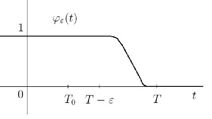
Let the sound speed $c(x)$ satisfy the conditions described in Section 2.1, namely, $c(x)>c>0,\;c(x)\in C^{\infty}(\mathbb{R}^{n})$, $c(x)-1$ has a compact support and $c(x)$ is non-trapping. Suppose also that the initial pressure $f(x)$ belongs to $L^{2}(\mathbb{R}^{n})$ and is compactly supported (in $B$). Then the following theorem, which is the main result of this article, holds.

Proof.   Let $E\colon H^{s}(S)\rightarrow H^{s+1/2}(B)\;,s>0,$ be the operator of harmonic extension that produces a harmonic function $E\phi$ in $B$ from the Dirichlet boundary data $\phi$ (e.g. [25]). Then $w\colon=e-Eg_{\varepsilon}$ satisfies

$$\left\{\begin{array}[]{l}w_{tt}-c^{2}(x)\Delta w=-{Eg_{\varepsilon}}_{tt}\qquad\mbox{in}\;B\times[0,T]\\ w(x,T)=p(x,T)-Eg_{\varepsilon}(x,T)=p(x,T)-Eg(x,T)\\ w_{t}(x,T)=p_{t}(x,T)-{Eg_{\varepsilon}}_{t}(x,T)=p_{t}(x,T)-Eg_{t}(x,T)\\ w|_{S}(x,t)=0\quad\mbox{on}\;S\times[0,T],\end{array}\right.$$

(8)

As noted in Section 2.1, there exists a time $T_{0}$ after which the solution $p(x,t)$ to (1) is infinitely smooth in $\bar{B}\times[T,\infty)$ for any $T>T_{0}$. Let us choose such $T$ and let $\varepsilon$ be such that $T-\varepsilon>T_{0}$. Then the right hand side and the initial conditions of (8) are infinitely smooth functions. Indeed, $p(x,T)$ is smooth, as we discussed above. Recall that $g_{\varepsilon}$ is a smooth cut-off of the trace of $p(x,t)$. Moreover, it is supported in $[T-\varepsilon,T]$ – a time interval where $p(x,t)$ has already become infinitely smooth. Thus $Eg_{\varepsilon}(x,t)$ is a smooth function as well.

Next, we will apply the following theorem to the solution of (8).

We will verify that the conditions of Theorem 4 are satisfied by (8), noting that the compatibility conditions must hold at $t=T$, since the direction of time is reversed. Indeed, as we already discussed, $F=-{Eg_{\varepsilon}}_{tt}$, $G=p(x,T)-Eg(x,T)$ and $H=p_{t}(x,T)-Eg_{t}(x,T)$ are infinitely smooth. It is clear that $G_{0}=G$ and $H_{1}=H$ belong to $H_{0}^{1}(\bar{B})$, as $g(x,t)$ has been defined to be the trace of $p(x,t)$. The higher order compatibility conditions hold as well:

$$\begin{array}[]{l@{\,}l}G_{2l}(x)=&-\frac{d^{2l-2}}{dt^{2l-2}}{Eg_{\varepsilon}}_{tt}(x,T)+c^{2}\Delta G_{2l-2}=-E\frac{d^{2l}}{dt^{2l}}{g}(x,T)+c^{2}\Delta G_{2(l-1)}\\ &=-E\frac{d^{2l}}{dt^{2l}}{g}(x,T)+(c^{2}\Delta)^{l}G_{0}=-E\frac{d^{2l}}{dt^{2l}}{g}(x,T)+(c^{2}\Delta)^{l}p(x,T).\end{array}$$

We used here that $\Delta E=0$.

As we already know that $p(x,T)$ is smooth in a neighborhood of $T$, we conclude that

$$\left.G_{2l}(x)\right|_{S}=\left.\left[-\frac{d^{2l}}{dt^{2l}}{p}(x,T)+(c^{2}\Delta)^{l}p(x,T)\right]\right|_{S}=0,$$

so $G_{2l}\in H^{1}_{0}(B)\mbox{ for }l=1,2...$ Similarly, one can check that $H_{2l+1}\in H^{1}_{0}(B)\mbox{ for }l=1,2...$.

Before applying Theorem 4 to the solution of (8) we notice that the energy in $B$, defined by $\mathscr{E}(t):=\frac{1}{2}\int_{B}\left(\left|\nabla w\right|^{2}+c^{-2}(x)\left|w_{t}\right|^{2}\right)dx$, stays constant in $[0,T-\alpha]$, where $\alpha=\min\{\varepsilon,1\}$. Indeed, using (8) one easily shows that

$$\dot{\mathscr{E}}(t)=\int_{B}\left(\nabla w\cdot\nabla w_{t}+c^{-2}w_{t}w_{tt}\right)\;dx=-\int_{B}w_{t}c^{-2}E{g_{\varepsilon}}_{tt}\;dx.$$

The last integral vanishes in $[0,T-\alpha]$, because ${g_{\varepsilon}}_{tt}\equiv 0$ in $[0,T-\alpha]$ and therefore, $E{g_{\varepsilon}}_{tt}\equiv 0$ in this interval. Then, by Theorem (4), it follows that

$$\begin{array}[]{l@{\!}l}\displaystyle\max_{0\leq t\leq T}\mathscr{E}(t)=\max_{T-\alpha\leq t\leq T}\mathscr{E}(t)\leq C\max_{T-\alpha\leq t\leq T}&\left\{\|w(t)\|^{2}_{H^{1}_{0}(B)}+\|w_{t}(t)\|^{2}_{L^{2}(B)}\right\}\leq\\ C\left\{\|{Eg_{\varepsilon}}_{tt}\|^{2}_{L^{2}(T-\alpha,T;L^{2}(B))}\right.+\|p(\cdot,T)-&Eg(\cdot,T)\|^{2}_{H_{0}^{1}(B)}\\ &+\left.\|p_{t}(\cdot,T)-Eg_{t}(\cdot,T)\|^{2}_{L^{2}(B)}\right\},\end{array}$$

where $C$ depends on $c(x)$ and $B$ only, but not on $T$ or $\varepsilon$. Here and in what follows $C$ will denote various constants, all of them independent on $T$ or $\varepsilon$.

As $w=e-Eg_{\varepsilon}$, the above inequalities imply

$$\begin{array}[t]{l}\displaystyle\max_{0\leq t\leq T}(\|e(t)\|_{H^{1}(B)}+\|e_{t}(t)\|_{L^{2}(B)})\leq\\ C\displaystyle\max_{0\leq t\leq T}\bigg\{\sqrt{\mathscr{E}(t)}+\|Eg_{\varepsilon}(t)\|_{H^{1}(B)}+\|{Eg_{\varepsilon}}_{t}(t)\|_{L^{2}(B)}\bigg\}\leq\\ \displaystyle C\bigg\{\max_{T-\alpha\leq t\leq T}(\|Eg_{\varepsilon}(t)\|_{H^{1}(B)}+\|{Eg_{\varepsilon}}_{t}(t)\|_{L^{2}(B)})+\|{Eg_{\varepsilon}}_{tt}\|_{L^{2}(T-\alpha,T;L^{2}(B))}\\ \mbox{\hskip 50.0pt}+\|p(\cdot,T)-Eg(\cdot,T)\|_{H_{0}^{1}(B)}+\|p_{t}(\cdot,T)-Eg_{t}(\cdot,T)\|_{L^{2}(B)}\bigg\}.\end{array}$$

(11)

We used here that $Eg_{\varepsilon}\equiv 0$ in $[0,T-\alpha]$.

Let $\mathcal{T}\colon H^{s}(B)\rightarrow H^{s-1/2}(S),s>1/2,$ denote the trace operator, which is known to be continuous (e.g.[26]). Then, using the continuity of the linear operators $E$ and $\mathcal{T}$, we can estimate the terms in (11) as follows.

$$\begin{array}[]{lr}\|Eg_{\varepsilon}(t)\|_{H^{1}(B)}\leq&C\|{g_{\varepsilon}(t)}\|_{H^{1/2}(S)}=C\|(1-\varphi_{\varepsilon}(t))\mathcal{T}p(t)\|_{H^{1/2}(S)}\leq\\ &C\|(1-\varphi_{\varepsilon}(t))p(t)\|_{H^{1}(B)}\leq C\|p(t)\|_{H^{1}(B)}.\end{array}$$

Similarly,

$$\begin{array}[]{lr}\|{Eg_{\varepsilon}}_{t}(t)\|_{L^{2}(B)}\leq&\|{Eg_{\varepsilon}}_{t}(t)\|_{H^{1}(B)}\leq C\|[(1-\varphi_{\varepsilon})p(t)]_{t}\|_{H^{1}(B)}\leq\\ &\displaystyle\frac{C}{\alpha}\left\{\|p(t)\|_{H^{1}(B)}+\|p_{t}(t)\|_{H^{1}(B)}\right\},\end{array}$$

$$\begin{array}[]{r}\|{Eg_{\varepsilon}}_{tt}(t)\|_{L^{2}(B)}\leq\|{Eg_{\varepsilon}}_{tt}(t)\|_{H^{1}(B)}\leq C\|[(1-\varphi_{\varepsilon})p]_{tt}\|_{H^{1}(B)}\leq\\ \displaystyle\frac{C}{\alpha^{2}}\left\{\|p(t)\|_{H^{1}(B)}+\|p_{t}(t)\|_{H^{1}(B)}+\|p_{tt}(t)\|_{H^{1}(B)}\right\},\end{array}$$

$$\|{Eg(T)}\|_{H^{1}(B)}\leq C\|{p(T)}\|_{H^{1}(B)}\mbox{ and }\|{Eg_{t}(T)}\|_{L^{2}(B)}\leq C\|{p_{t}(T)}\|_{H^{1}(B)}.$$

Here we used that $\displaystyle\max_{t}|\varphi_{\varepsilon}^{\prime}(t)|\leq C^{\prime}/\alpha$ and $\displaystyle\max_{t}|\varphi_{\varepsilon}^{\prime\prime}(t)|\leq C^{\prime\prime}/\alpha^{2}$ for some constants $C^{\prime}$ and $C^{\prime\prime}$. Then, the error can be estimated by

$$\begin{array}[]{l}\displaystyle\max_{0\leq t\leq T}\left\{\|e(t)\|_{H^{1}(B)}+\|e_{t}(t)\|_{L^{2}(B)}\right\}\leq\\ \displaystyle\frac{C}{\alpha^{2}}\left\{\max_{T-\alpha\leq t\leq T}\left(\|p(t)\|_{H^{1}(B)}+\|p_{t}(t)\|_{H^{1}(B)}\right)+\right.\\ \mbox{\hskip 15.0pt}\quad\|p\|_{L^{2}(T-\alpha,T;H^{1}(B))}+\|p_{t}\|_{L^{2}(T-\alpha,T;H^{1}(B))}+\|p_{tt}\|_{L^{2}(T-\alpha,T;H^{1}(B))}+\\ \mbox{\hskip 200.0pt}\|p(T)\|_{H^{1}(B)}+\|p_{t}(T)\|_{H^{1}(B)}\Bigg\}\end{array}$$

(12)

Theorem 2 allows us to estimate the quantity inside the braces in right-hand side of above inequality by a factor of

$$\begin{array}[]{l}\displaystyle\bigg\{\max_{T-\alpha\leq t\leq T}\left[\eta_{0}(t)+\eta_{1}(t)\right]+\|\eta_{0}\|_{L^{2}(T-\alpha,T)}+\|\eta_{1}\|_{L^{2}(T-\alpha,T)}\\ \mbox{\hskip 100.0pt}+\|\eta_{2}\|_{L^{2}(T-\alpha,T)}+\eta_{0}(T)+\eta_{1}(T)\bigg\}\|f\|_{L^{2}(B)}\end{array}$$

The functions $\eta_{k}(t)$ are monotonically decreasing, and $\eta_{2}(t)\leq\eta_{1}(t)\leq\eta_{0}(t)$ provided $t\geq 1$. Therefore, the right hand side of (12) is less than

$$C/\alpha^{2}\left\{\eta_{0}(T-\alpha)+\|\eta_{0}\|_{L^{2}(T-\alpha,T)}\right\}\|f\|_{L^{2}(B)}.$$

Taking into account that

$$\|\eta_{0}\|^{2}_{L^{2}(T-\alpha,T)}\leq\alpha\max_{T-\varepsilon\leq t\leq T}\eta^{2}_{0}(t)\leq\eta^{2}_{0}(T-\varepsilon),$$

we arrive to

$$\max_{0\leq t\leq T}(\|e(t)\|_{H^{1}(B)}+\|e_{t}(t)\|_{L^{2}(B)})\leq C(\varepsilon)\eta_{0}(T-\varepsilon)\|f\|_{L^{2}(B)},$$

where $\eta_{0}(T-\varepsilon)=(T-\varepsilon)^{-n+1}$ for even n, $\eta_{0}(T-\varepsilon)=e^{-\delta(T-\varepsilon)}$ for odd n, and $C(\varepsilon)=C/\min\{\varepsilon^{2},1\}$.

This proves the theorem.

In this section we compare the errors of the numerical reconstructions of several phantoms to their estimates given in Theorem 3. The numerical simulations were done in 2D media with variable sound speed. Both cases of non-trapping and trapping sound speed are considered.

For the computations we used the rectilinear finite difference scheme (as in [16, 12]), implemented in Matlab. For both simulation of the phantom data and reconstruction, we approximated the boundary of the unit circle, $S$, by the set of grid points closest to $S$ and lying within $B$. For the simulation of phantom data the following problem was solved

$$\left\{\begin{array}[]{l}p_{tt}-c_{0}^{2}\Delta p=0\qquad\mbox{in}\quad D\times(0,T_{0}]\\ p(x,0)=f(x)\;p_{t}(x,0)=0\\ p|_{\partial D}=0,\end{array}\right.$$

where $D=[-a,a]^{2}$ was a square containing $S$ and large enough to ensure that no reflections off its boundary would reach $S$ for time $T_{0}$. The values of the solution on $S$ were recorded for all time steps. The time $T_{0}$, the domain $D$ and the space and time step-sizes were adjusted depending on the situation. For the reconstruction part, the same equation and difference scheme (but a different mesh) were used, this time on the square $[-1.2,1.2]^{2}$ instead of on $D$. To obtain the values of the boundary data at the grid points used for reconstruction we used nearest point approximation. In order to observe the behavior of the error of reconstruction with respect to the cut-off time $T$, multiple reconstructions from different cut-off times were made and the error was graphed on a logarithmic scale. In both forward simulation and reconstruction, the spatial step-size $h$ varied case by case and was of the order of $10^{-2}$. This corresponds to using several hundred detectors on the boundary of the unit circle.

On Figure 2 examples of reconstructions using the time reversal method are shown. In the first case a variable non-trapping speed was used and the reconstruction is of a high quality. In the second example, the radial sound speed equals $|x|$ in the annulus $A=\{x|0.5<|x|<1\}$ and is constant elsewhere. This ”trapping crater” speed traps all rays corresponding to bicharacteristics that start at points $(x_{0},\xi_{0})$ such that $x_{0}\in A$ and $x_{0}\perp\xi_{0}$. The trapping leads to the blurring of the radial sides of the phantom, since those singularities do not reach the observation surface. A discussion of this phenomenon can be found in [12]. In the third example, shown in Figure 2, the sound speed equals $|x|^{2}+0.1$ inside the unit circle. This speed exhibits a more severe trapping than the “trapping crater“ speed, which leads to a much stronger blurring. In this case, for any $x_{0}$ there exists a cone of directions $\xi_{0}$, such that the ray corresponding to the bicharacteristic starting at $x_{0},\xi_{0}$ is trapped [27].

In the next two figures we present various sound speeds and analyse the errors of reconstruction as functions of the cut-off time $T$. These figures show the particular sound speed, phantoms and the corresponding errors, but not actual reconstructions, as we have already seen examples of such in Figure 2. The plot of each error shows only values of the error after some minimal time, specific to each sound speed, after which it makes sense to apply the time reversal procedure. Namely, this minimal time is taken to be the time a wave needs to cross the unit circle. After the error has decreased to a very small value it levels off, which is due to the discretization of the model. Thus, the error plots do not show these values. In order to easily observe the behaviour of the error, the plots are made in a logarithmic scale and the corresponding linear regression interpolations are graphed.

Figures 3 and 4 show two examples of variable non-trapping sound speeds. In both cases two different phantoms are considered and the $H^{1}$ error of reconstruction as a function of the cut-off time $T$ is plotted. In Theorem 3 we estimated that, in two dimensions, the error behaves as $T^{-1}$. The examples from Figures 3 and 4 suggest even faster decay for those particular sound speeds. In the case shown in Figure 3 the $H^{1}$ error decays as $T^{-1.3}$. The decay of the error in the second example (Figure 4) is even faster: the plots suggest that it is of the order of $T^{-1.6}$. The next two examples deal with trapping sound speeds. In these cases the behaviour of the error depends also on the initial condition, as there is no uniform local energy decay unless additional smoothness is assumed (e.g. [28, 29]). The $L^{2}$ errors shown in Figures 5 and 6 decay as $T$ increases.

• •

  In this text, we have concentrated on the errors resulting from the time reversal approximation. One is also interested in the stability of the method with respect to errors in the data. This question is answered by the standard results on stability of the mixed problem for the wave equation. If $n(x,t)$ is the error in the measured data $g(x,t)$, then a stability estimate should bound a norm of $\tilde{e}(x,0;T)$, where $\tilde{e}(x,t;T)$ solves the following mixed value problem:

  $$\left\{\begin{array}[]{l}\tilde{e}_{tt}(x,t;T)=c^{2}(x)\Delta\tilde{e}(x,t;T)\qquad\mbox{in}\;B\times[0,T]\\ \tilde{e}(x,T;T)=0\\ \tilde{e}_{t}(x,T;T)=0\\ \tilde{e}|_{S}(x,t;T)=n_{\varepsilon}(x,t)\colon=(1-\varphi_{\varepsilon}(t))n(x,t)\qquad\mbox{in}\;S\times[0,T].\end{array}\right.$$

  (13)

  Since $c(x)$ is assumed to be smooth, classical results (e.g. [30, Ch. 5, Sec. 5]) give, for instance, the following estimate:

  $$\|\tilde{e}(x,0;T)\|_{L^{2}(B)}\leq C\|n(x,t)\|_{H^{1+\delta,1+\delta}([0,T]\times S)}$$

  Here $H^{1+\delta,1+\delta}([0,T]\times S)=L^{2}(0,T;H^{1+\delta}(S))\cap H^{1+\delta}(0,T;L^{2}(S))$ and $\delta>0$. In a nutshell, the reconstruction is as stable as Radon inversion in the corresponding dimension.

• •

  Our numerical examples show decay of the error also in the trapping speed case. One could probably get some estimates on this decay, assuming sufficient smoothness of the function $f(x)$ to be reconstructed and using the results of [29]. It is unlikely that one can get such estimates without a smoothness assumption.

To conclude, in this paper we have provided error estimates of the time reversal justifying it in any dimension under non-trapping condition. The numerical examples agree with the error estimates in the cases of non-trapping speeds and show that the time reversal works even when the speed is trapping.

References

- [1] A C Tam. Applications of photoacoustic sensing techniques. Reviews of Modern Physics, 58(2):381–431, 1986.
- [2] M Xu and L V Wang. Photoacoustic imaging in biomedicine. Review of Scientific Instruments, 77:041101, 2006.
- [3] M Xu and L V Wang. Time-domain reconstruction for thermoacoustic tomography in a spherical geometry. Medical Imaging, IEEE Transactions on, 21(7):814–822, 2002.
- [4] L V Wang and H Wu. Biomedical Optics. Principles and Imaging. Wiley-Interscience, New York, 2007.
- [5] G J Diebold, T Sun, and M I Khan. Photoacoustic monopole radiation in one, two, and three dimensions. Physical Review Letters, 67(24):3384–3387, 1991.
- [6] P Kuchment and L Kunyansky. Mathematics of thermoacoustic tomography, 2008.
- [7] D Finch and Rakesh. The spherical mean value operator with centers on a sphere. Inverse Problems, 23(6):S37–S49, 2007.
- [8] M Agranovsky, P Kuchment, and L Kunyansky. On reconstruction formulas and algorithms for the thermoacoustic and photoacoustic tomography. In L H Wang, editor, Photoacoustic imaging and spectroscopy, pages 89–101. CRC Press, 2009.
- [9] D Finch and Rakesh. Recovering a function from its spherical mean values in two and three dimensions. In L H Wang, editor, Photoacoustic imaging and spectroscopy. CRC Press, 2009.
- [10] S Patch and O Scherzer. Guest editors’ introduction: Photo- and thermo-acoustic imaging. Inverse Problems, 23(6):S1–S10, 2007.
- [11] M. Haltmeier, T. Schuster, and O. Scherzer. Filtered backprojection for thermoacoustic computed tomography in spherical geometry. Math. Methods Appl. Sci., 28(16):1919–1937, 2005.
- [12] Y Hristova, P Kuchment, and L Nguyen. Reconstruction and time reversal in thermoacoustic tomography in acoustically homogeneous and inhomogeneous media. Inverse Problems, 24(055006):055006, 2008.
- [13] M Fink and C Prada. Acoustic time-reversal mirrors. INVERSE PROBLEMS, 17(1):1–38, 2001.
- [14] M Fink. Time-reversal acoustics. Journal of Physics: Conference Series, 118:012001 (28pp), 2008.
- [15] P Blomgren, G Papanicolaou, and H Zhao. Super-resolution in time-reversal acoustics. The Journal of the Acoustical Society of America, 111:230, 2002.
- [16] P Burgholzer, G J Matt, M Haltmeier, and G Paltauf. Exact and approximative imaging methods for photoacoustic tomography using an arbitrary detection surface. Physical Review E, 75(4):46706, 2007.
- [17] H Grün, G Paltauf, M Haltmeier, and P Burgholzer. Photoacoustic tomography using a fiber based Fabry-Perot interferometer as an integrating line detector and image reconstruction by model-based time reversal method. Proceedings of SPIE, 6631:663107, 2007.
- [18] L Nirenberg. Lectures on linear partial differential equations. American Mathematical Society, Providence, R.I., 1973. Expository Lectures from the CBMS Regional Conference held at the Texas Technological University, Lubbock, Tex., May 22–26, 1972, Conference Board of the Mathematical Sciences Regional Conference Series in Mathematics, No. 17.
- [19] Michael E. Taylor. Pseudodifferential operators, volume 34 of Princeton Mathematical Series. Princeton University Press, Princeton, N.J., 1981.
- [20] Y V Egorov and M A Shubin. Linear partial differential equations. Foundations of the classical theory. In Partial differential equations, I, volume 30 of Encyclopaedia Math. Sci., pages 1–259. Springer, Berlin, 1992.
- [21] B R Vainberg. The short-wave asymptotic behavior of the solutions of stationary problems, and the asymptotic behavior as of the solutions of nonstationary problems. Uspehi Mat. Nauk, 30(2(182)):3–55, 1975. English translation: Russian Math. Surveys 30 (1975), no. 2, 1–58.
- [22] J V Ralston. Solutions of the wave equation with localized energy. Comm. Pure Appl. Math., 22:807–823, 1969.
- [23] R Pauen. Non-trapping Conditions and Local Energy Decay for Hyperbolic Problems. volume 132 of Konstanzer Schriften in Mathematik und Informatik. preprint, http://www.ub.uni-konstanz.de/kops/volltexte/2006/2146/, 2006.
- [24] R Courant and D Hilbert. Methods of mathematical physics. Vol. II: Partial differential equations. (Vol. II by R. Courant.). Interscience Publishers (a division of John Wiley & Sons), New York-Lon don, 1962.
- [25] J L Lions and E Magenes. Non-homogeneous boundary value problems and applications. Vol. 1. Springer-Verlag, New York, 1972.
- [26] L C Evans. Partial differential equations, volume 19 of Graduate Studies in Mathematics. American Mathematical Society, Providence, RI, 1998.
- [27] L Nguyen. Singularities and instability in thermoacoustic tomography. preprint, 2008.
- [28] J Ralston. Gaussian beams and the propagation of singularities. In Studies in partial differential equations, volume 23 of MAA Stud. Math., pages 206–248. Math. Assoc. America, Washington, DC, 1982.
- [29] N Burq. Décroissance de l’énergie locale de l’équation des ondes pour le problème extérieur et absence de résonance au voisinage du réel. Acta Math., 180(1):1–29, 1998.
- [30] J L Lions and E Magenes. Non-homogeneous boundary value problems and applications. Vol. II. Springer-Verlag, New York, 1972.