Non-linear Evolution of Cosmologies III: Halo Statistics
Abstract
The statistical properties of dark matter halos, the building blocks of cosmological observables associated with structure in the universe, offer many opportunities to test models for cosmic acceleration, especially those that seek to modify gravitational forces. We study the abundance, bias and profiles of halos in cosmological simulations for one such model: the modified action theory. The effects of modified gravity can be separated into a large- and small-field limit. In the large field limit, which is accessible to current observations, enhanced gravitational forces raise the abundance of rare massive halos and decrease their bias but leave their (lensing) mass profiles largely unchanged. This regime is well described by scaling relations based on a modification of spherical collapse calculations. In the small field limit, the enhancement of the gravitational force is suppressed inside halos and the effects on halo properties are substantially reduced for the most massive halos. Nonetheless, the scaling relations still retain limited applicability for the purpose of establishing conservative upper limits on the modification to gravity.
I Introduction
In the so-called class of models (see [1, 2] and references therein) cosmic acceleration arises not from an exotic form of energy with negative pressure but from a modification of gravity that replaces the Einstein-Hilbert action by a function of the Ricci or curvature scalar [3, 4, 5].
Cosmological simulations are crucial for exposing the phenomenology of models. In order to satisfy local tests of gravity, models exhibit a non-linear process, called the chameleon mechanism, to suppress force modifications in the deep potential wells of cosmological structure [6, 7, 8, 9, 10]. Upcoming tests of cosmic acceleration from gravitational lensing, galaxy and cluster surveys have most of their statistical weight in the weakly to fully non-linear regime. Stringent constraints on modified gravity can be expected from current and future surveys, once the impact on observables in the non-linear regime is understood.
In the previous papers in this series, we have established the methodology for cosmological simulations [11] and conducted a suite of simulations that uncover the chameleon mechanism and its effect on the matter power spectrum [12]. In this paper, we continue our exploration of the non-linear aspects of the model by examining the properties of the basic building blocks of cosmological structure: dark matter halos. Specifically, we quantify their abundance, i.e. the halo mass function, clustering properties, i.e. the linear bias, and their density profiles, to see how each are modified from the standard cosmological constant, cold dark matter model CDM.
We begin in §II with a brief review of the important properties of models and a discussion of the simulation and analysis methodology. We present our results on halo statistics in §III and discuss them in §IV. Throughout we place a special emphasis on exploring the impact of the chameleon mechanism and highlighting differences between the simulations and conventional scaling relations based on linear theory and CDM. These differences expose crucial distinctions that must be considered when observationally testing modified gravity theories.
II Methods
We begin in §II.1 by briefly reviewing the basic properties of the model that are important for understanding the cosmological simulations described in §II.2. We refer the reader to [12] for a more detailed treatment. Finally in §II.3, we discuss the methods used in identifying the halos and measuring their abundance, bias and profiles.
II.1 Gravity
The model generalizes the Einstein-Hilbert action to include an arbitrary function of the scalar curvature ,
| (1) |
Here is the Lagrangian of the ordinary matter and throughout . Force modifications are associated with an additional scalar degree of freedom . For definiteness, we choose the functional form for given in [10] (with ), but neglect higher corrections of order which results in the following effective :
| (2) |
Here we define and , where overbars denote the quantities of the background spacetime. For the background expansion history mimics CDM with .
Variation of Eq. (1) with respect to the metric yields the modified Einstein equations. We work in the quasistatic limit, where time derivatives may be neglected compared with spatial derivatives. The trace of the modified Einstein equations yields the field equation
| (3) |
where coordinates are comoving, , , . The time-time component of the Einstein equations yields the modified Poisson equation
| (4) |
Here is the Newtonian potential or time-time metric perturbation in the longitudinal gauge. These two equations define a closed system for the Newtonian potential given the density field. The matter falls in the Newtonian potential as usual and so the modifications to gravity are completely contained in the equation for .
The field equation (3) is a non-linear Poisson-type equation, where the non-linearity is determined by . If the background field is sufficiently large, then field fluctuations are relatively small and this term may be linearized as . It is straightforward to show that the Fourier space solution to Eqs. (3) and (4) in this approximation is
| (5) |
with . Hence, gravitational forces are enhanced by a factor of on scales below , the Compton wavelength of the field. We call this regime the large field limit.
Eqs. (3) and (4) in the large field limit imply that the field fluctuations are of order the gravitational potential . Therefore if the background field is of order the typical gravitational potentials of cosmological structure or smaller, field fluctuations become of order unity and which causes the Compton wavelength to shrink [10]. We call this the small field limit. The large and small field limits are separated by a value of the background field of .
In the small field limit, the field equation (3) then requires which drives the Poisson equation (4) back to its usual form. This is the so-called chameleon mechanism which occurs when the background field is small compared with the depth of the gravitational potential. Hence force law deviations are suppressed in the deepest gravitational potentials, i.e. inside the high overdensities of collapsed dark matter halos.
II.2 Simulations
To solve the system of equations defined by the modified Poisson equation (4) and the field equation (3) in the context of cosmological structure formation, we employ the methodology described in [11] and implemented in [12]. Briefly, the field equation for is solved on a regular grid using relaxation techniques and multigrid iteration [13, 14]. The potential is computed from the density and fields using the fast Fourier transform method. The dark matter particles are then moved according to the gradient of the computed potential, , using a second order accurate leap-frog integrator.
We choose a range of background field values to expose the impact of the chameleon mechanism. Since cosmological potentials range from , we expect the chameleon mechanism to be operative in the small field limit of this range but absent in the large field limit. We also include which is equivalent to CDM. Note that the background expansion history for all runs are indistinguishable from CDM to . More specifically, we take a flat background cosmology defined by , , km/s/Mpc and initial power in curvature fluctuations at Mpc-1 with a tilt of .
To more directly assess the impact of the chameleon mechanism, we also carry out linearized simulations in which the gravitational potential, , is evaluated according to Eq. (5). In the linearized treatment, the Compton wavelength is assumed to be fixed by the background field and thus chameleon effects are not present. Therefore, the difference between the full simulations and the linearized simulations are wholly due to the chameleon effects. We will call these runs the “no-chameleon” simulations.
Table 1 lists the properties of the simulations used in the analysis below. All simulations possess 512 grid cells in each direction and particles.
| ( Mpc) | |||||
| # of | 6 | 6 | 6 | 6 | |
| boxes | 6 | 6 | 6 | 6 | |
| 6 | 6 | 6 | 6 | ||
| 0 (CDM) | 6 | 6 | 6 | 6 | |
| () | 204 | 53.7 | 6.61 | 0.83 | |
| ( Mpc-1) | 0.008 | 0.012 | 0.025 | 0.049 | |
| ( Mpc) | 0.78 | 0.50 | 0.25 | 0.125 | |
II.3 Halo Properties
We identify halos and measure their masses in simulations with a spherical overdensity algorithm similar to [15]. We use cloud-in-cell interpolation to assign the particles to the grid. Starting at the highest overdensity grid point, we then count the particles within a growing sphere centered on the center of mass, until the desired overdensity with respect to the mean matter density is reached. Here, we take for definiteness. The mass of the halo is then defined by the mass of all particles enclosed within this radius . We move onto the next highest density grid cell and repeat the procedure until all halos have been identified. We implicitly take below unless otherwise specified.
In our final results we only keep halos with at least dark matter particles, and since our simulations are not of high-resolution, we conservatively take . We verified that a lower minimum particle number of provides results consistent with statistical uncertainties for all our quoted halo properties. The corresponding minimum masses of halos are listed in Table 1.
For each simulation run, we determine the halo mass function by binning halos in logarithmic mass intervals, and dividing by the comoving volume of the simulation box. We then combine different runs and box sizes using a bootstrap procedure to produce the estimate of the mass function and its errors. We weight each box by volume and use only those boxes whose minimum halo mass is below the mass bin considered. When measuring differences between CDM and , we average the differences between simulations with the same initial conditions to reduce the sample variance.
We compare simulation results to the Sheth-Tormen (ST) prescription [16] given in Appendix B with modifications to spherical collapse as detailed in the Appendix A. Semi-analytic prescriptions of this type are widely used when analyzing data for cosmological constraints and so an assessment of their range of validity is of practical importance.
Next we extract the linear halo bias from our simulations. For halos of a given logarithmic mass range in a box of size , we first obtain the halo bias by dividing the halo-mass cross spectrum by the matter power spectrum for each simulation
| (6) |
where is the halo number density contrast whereas is the matter mass density contrast. The average is over the -modes in a -bin. For each box we employ the modes , where is the fundamental mode of the box (see Table 1) and thus the smallest boxes barely probe the linear regime. For the larger mass bins, we probe more of the linear regime but are more limited by small statistical samples. Note that the definition of bias adopted will differ from alternate choices such as or in the non-linear regime where the correlation coefficient between halos and matter can differ from unity.
In order to remove trends from the non-linearity of the bias, we fit a linear relation to between and , where is the combined measurement from all boxes. The linear halo bias in this mass range is then extrapolated as . When considering the modifications in the simulations, the same bootstrap and linear fit procedure is applied but to the quantity . Again we compare these results to the peak-background split predictions based on the ST mass function detailed in Appendix B.
Finally, we stack the halos in each mass interval and measure the average density profile and mass correlations of the halos. To reduce scatter within the mass bin we scale each density profile to its own before stacking, i.e. we measure
| (7) |
The spatial resolution of our particle-mesh simulations is limited by the fixed size of grid cells (see Tab. 1). We measure halo profiles down to the grid scale, though we expect that profiles have converged only at scales of several grid cells. When the resolution becomes too low, the inner profile flattens leading to a misestimation of both the mass enclosed at and the shape of the halo profiles. We therefore use only the highest resolution boxes for our comparisons with the simulations. The maximum radius for each profile is set to .
In order to avoid biases from incompleteness effects, we further limit the range of the stacked profile to radii where more than 90% of the halos in the mass bin contribute. We then bootstrap over all halos in the given mass range in order to determine the average profile and its error. Profiles and the halo-mass correlation function results are compared to the Navarro-Frenk-White (NFW) profile and halo model respectively (see Appendix B).


III Results
In this section we present the results obtained from N-body simulations of the models for the halo mass function (§III.1), halo bias (§III.2), density profiles (§III.3) and matter power spectrum (§III.4). In all cases, we compare the simulation results with predictions using scaling relations based on spherical collapse calculations, the Press-Schechter prescription and findings from simulations of CDM. These calculations are detailed in the Appendices.
Since spherical collapse predictions depend on the gravitational force modification, we give a range of predictions in each case. The extremes are given by collapse with standard gravity and with enhanced forces throughout. The former follows the CDM expectation of a linear density extrapolated to collapse of and a virial overdensity of ; the latter modifies these parameters to and as detailed in Appendix A.
Neither assumption for the nonlinear collapse is completely valid given the evolving Compton wavelength and the chameleon mechanism. Moreover, the evolution of linear density perturbations used as the reference for the scaling relations in Eqs. (25), (28), (32), and (34) assumes in both cases the full linear growth of the model through , including the effects of the evolving background Compton wavelength but not the chameleon mechanism. Thus unmodified spherical collapse parameters do not equate to unmodified spherical collapse predictions.


III.1 Mass Function
In Fig. 1, we show the halo mass function measured from our suite of CDM simulations along with the bootstrap errors described in §II.3. For reference, we compare the simulations to the Sheth-Tormen (ST) mass function of Eq. (25). The ST formula gives the mass function in terms of the virial mass and we rescale it to assuming an NFW profile (see Appendix B). Our CDM simulations are consistent with the 10-20% level of accuracy expected of the ST formula and internally between boxes of differing resolution.
Next, we compare the and CDM simulations. Our measurement of the halo mass function itself is limited by statistics and to a lesser extent, resolution (see Fig. 1). However, we can reduce the impact of both effects by considering the relative difference between the halo mass functions measured in and CDM simulations with the same initial conditions and resolution.
Fig. 2 shows this relative enhancement of the halo mass-function in the simulations for different values of , the background field today, combining different box sizes as described in section II.3. We show results for the full simulations as well as the no-chameleon simulations to help highlight the impact of the chameleon mechanism.
For the large field value of , the number of halos increases significantly, especially at the high mass end, by up to 50150% for cluster-sized halos. The chameleon effect slightly suppresses the abundance in the high mass end. A similar effect occurs for the power spectrum [12] and arises due to the appearance of the chameleon effect in deep potentials at high redshifts where the background field values are smaller. The overall trend is captured by the spherical collapse predictions (shaded band in Fig. 2). The upper limit corresponds to unmodified forces, whereas the lower limit corresponds to enhanced forces during the entirety of the collapse. The enhancement of the linear in effectively makes objects of the same mass less rare and causes the increase in the Sheth-Tormen predictions for the exponentially suppressed high-mass end of the mass function (). Compared to this effect, that of modifying spherical collapse parameters is much smaller. It mainly arises from the increase in virial mass with respect to making the same correspond to rarer virialized objects. In this large field limit, all but the most massive halos are better described by the modified collapse parameters. Moreover, for the purposes of establishing upper limits on using the halo mass function, use of this prediction would only err on the conservative side.
When the value of the field becomes comparable to the cosmological potential wells, the chameleon effect starts to operate. This can be seen in the mass function deviations for and (see Fig. 2). For the smallest field value, the departures from CDM become very small, so that individual high-mass halos change only slightly in mass. Due to the limited statistics in our simulation sample, we are not able to reliably estimate the uncertainties on the mass function deviation for the highest mass bin in this case. However, the mean deviation in this mass bin is consistent with zero.
The no-chameleon simulations show a behavior of increasing deviations at high masses similar to the large-field case, while the full simulations deviate significantly from this trend, especially at high masses. For the excess almost entirely disappears at the highest masses leaving a pile-up of halos at intermediate masses. As in the power spectrum [12], the chameleon mechanism qualitatively changes the predictions for the mass function for .
It is also apparent from Fig. 2 (lower panel) that the spherical collapse predictions are less accurate for the small field limit. The range of predictions encompasses a deficit of high mass halos that is not seen in the simulations. Since is calculated from the linear prediction at a radius that encloses the mass at the background density, there would be no predicted enhancement of linear fluctuations if this radius is larger than the Compton scale in the background. This is in spite of the fact that in the no-chameleon simulations forces are still enhanced once the perturbation collapses to smaller scales. Combined with the rescaling of the virial mass, this can produce a deficit of predicted objects at a fixed overdensity. This problem highlights the difficulties in applying scaling relations between the linear and non-linear regime, which were developed for scale-free CDM type models, to modified gravity theories.
In the case of the full simulations, the problem is partially compensated by the appearance of the chameleon mechanism which also reduces the abundance of the highest mass objects by eliminating the extra force during the collapse. While the full simulation results lie within the range of spherical collapse predictions at the high mass end, spherical collapse fails to predict the pile up of halos at intermediate masses.
Still, the ST mass function predictions can be used to conservatively place upper limits on from the abundance of halos with . Employing the modified collapse prescription for the enhancement or zero, whichever is greater, will always underestimate the true enhancement in the suite of models we have tested. This underestimate becomes a small fraction of the total enhancement for .
III.2 Halo Bias
The halo bias computed from Eq. (6) in the CDM simulations is shown in Fig. 3 for halos with masses in the range as an example. The points and error bars are bootstrap averages and errors of individual bias computations from the various boxes and runs. In this case, only boxes with size and Mpc have halos in the mass range and contribute to the bias calculation (see Tab. 1). Note that due to the limited halo statistics and our small simulation sample, the scatter in the errors themselves is significant. We have verified that consistent results are also obtained with a lowered which increases halo statistics allowing the larger, more linear, boxes to be used for the bias. In the lower panel of Fig. 3 we show the variation of the bias measurements with box size. In the regime of mutual applicability, the bias measurements between boxes are consistent within the statistical uncertainties.
In Fig. 4, we show the linear halo bias in our CDM simulations as a function of halo mass, measured as described in §II.3. We compare these results to the ST bias prediction of Eq. (28). We again remap the virial mass to and plot the prediction for . The simulation results are consistent within of the prediction.


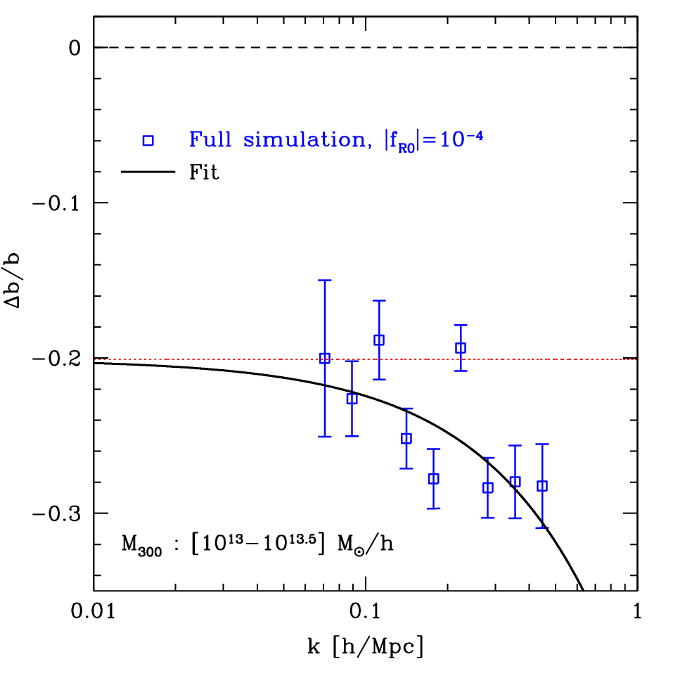
Whereas the abundance of halos can be significantly changed in , their clustering properties are relatively less affected compared with CDM. In Fig. 5 we show the relative difference between the halo bias in simulations with and CDM for the same mass bin of Fig. 3. For each box and run contribution, we subtracted the simulation bias from that of the corresponding CDM simulation with same initial conditions to form . The averages and error displayed are again obtained by bootstrap of the individual differences. The same linear fit procedure is applied and evaluated at to estimate the relative difference in the linear bias .
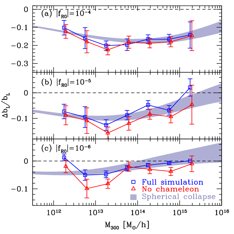
In Fig. 6 we compare the linear bias from and CDM simulations, computed as above, and the range of predictions from spherical collapse. The bias decreases with increasing since halos of a fixed mass become less rare and thus less highly biased. The chameleon effect in the full simulations decreases the difference in bias versus the no chameleon simulations as expected. As with the mass function, the spherical collapse range adequately describes the high mass halos even for the small-field chameleon cases due to a fortuitous cancellation of modeling errors.
III.3 Halo Profiles
The final ingredient in a basic understanding of halos and cosmological statistics that are built out of them is their average profiles. We plot the fractional density contrast defined in Eq. (7) and measured in the CDM simulations for the largest and hence best resolved mass bin in Fig. 7 (upper panel), for different box sizes of the CDM simulations. For reference we compare these with the corresponding halo model prediction (shaded) from the halo-mass correlation function of Eq. (35), consisting of an NFW profile plus a 2-halo term describing the surrounding mass, averaged over the same mass bin as the simulations. The range of predictions shown is bounded from above by a continued NFW profile, and bounded from below by an NFW profile truncated at as used in the halo model description of power spectra, Eq. (32). In the lower panel of Fig. 7, we show the same profiles relative to the halo model prediction with continued profiles. Removing the overall trend with the halo model better reveals the internal consistency of our simulations. The agreement between the smallest box and the larger boxes with coarser resolution and smaller particle number is % in case of the 128 boxes, and % for the 256 boxes. In the following, we show results from the 128 boxes for the largest mass halos, in order to increase halo statistics, and from the 64 boxes for all other masses.
Fig. 8, top panel, shows the stacked halo profiles for three mass bins, for CDM and full simulations with . The lower panel of Fig. 8 shows the relative deviation between CDM and halo profiles. When scaled to the same overdensity radius, halos in CDM and apparently have very similar profiles, especially in the inner part of the halo. Although a precise measurement of the NFW scale radius is not possible with our limited resolution, it is apparent that there are no dramatic effects of modified gravity on the halo concentration . Moreover the deviations are consistent with zero well within . The same holds for the no-chameleon simulations.
For the intermediate and larger halo masses, there is an enhancement of the halo profile at few, i.e. in the transition region between one-halo and two-halo contributions. The smallness of the enhancement of can be explained by a partial cancellation between the increased linear power spectrum and reduced linear bias in (§ B and § III.2). However, a quantitative understanding of the behavior of the halo-mass correlation at these radii is not possible with the simple halo model adopted here, as it fails in the transition region between one and two-halo terms (see Fig. 7). In the small field simulations, the deviations in the halo profiles are too small to be measured with our current suite of simulations.
Given the relative smallness of the modified gravity effects on halo profiles, the main effect of enhanced forces in the large field simulations is to change the mass and hence the abundance and bias of halos.

III.4 Halo Model Power Spectrum
We can now put the halo properties together and discuss statistics that can be interpreted under the halo model paradigm outlined in §B. The matter power spectrum is especially interesting in that the enhancement in the large field simulations found in [12] was not well described by standard linear to nonlinear scaling relations [22]. Without an adequate description of the large field limit, robust upper limits on , which should be available from current observations, are difficult to obtain.
The halo model provides a somewhat more physically motivated scaling relation between the linear and nonlinear power spectra [23]. Specifically we use the same range of ST predictions for the mass function and linear bias discussed in the previous sections in Eq. (32). In addition, we vary the concentration parameter of the halos, using either an unmodified relation [Eq. (30)], or an unmodified . The latter relation is motivated by our finding that the inner parts of halo profiles are unmodified in when referred to the same overdensity radius (§ III.3). Converting to the virial concentration, we obtain a 10% higher , which increases the power spectrum enhancement at through the 1-halo term [Eq. (32)].
The range of halo model predictions is shown in Fig. 9 for different values of , together with the simulation results from [12]. The upper boundary of each shaded band corresponds to unmodified spherical collapse parameters and unchanged , while the lower boundary is using the modified spherical collapse parameters, assuming enhanced forces throughout in the prediction, and unchanged .
The halo model provides a reasonable approximation to the relative deviations in the large field limit out to the /Mpc scales that can be resolved by the simulations. The modified collapse provide a somewhat better and more conservative approximation for the purposes of establishing upper limits for .
The halo model still fails to capture the chameleon suppression in the small field limit. Its failure is apparent even at for Mpc) and is relatively larger than the error in the mass function, linear bias and halo profiles themselves. This range also corresponds to the regime where the one halo and two halo terms are comparable, i.e. where our simple prescription of linear clustering of halos with density profiles truncated at the virial radius cannot be expected to apply.
A prescription that seeks to interpolate between modified and unmodified force law predictions [23] and a better treatment of the transition regime that includes nonlinear halo clustering and halo exclusion could potentially provide a better description but is beyond the scope of this study.
IV Discussion
Dark matter halos are the building blocks of cosmological observables associated with structure in the universe. Their statistical properties provide many interesting tests of cosmic acceleration, especially of those that seek to modify gravitational forces.
Here we have examined the abundance, clustering and profiles of dark matter halos in modified gravity models. In these models, gravitational forces are enhanced below the local Compton scale of an extra scalar degree of freedom . Generically, this extra force leads to an enhanced abundance of massive halos and a decrease in the bias of such halos, but relatively little change to the density profile or mass correlation around halos of fixed mass. The extent of these effects on halo statistics depends strongly on whether the background scalar field is in the large field () or small field limit ().
In the large field limit, forces are modified everywhere below the background Compton scale ( today [12]). The modifications in this regime are relatively well described by scaling relations for halo statistics. By modifying spherical collapse parameters to include the enhanced forces, we have shown that the mass function and linear halo bias can be described well by the Sheth-Tormen prescription. The halo-mass correlation and average density profiles are little changed from CDM due to a cancellation of effects from the enhanced forces and decreased bias.
Together these provide a description of the enhanced matter power spectrum that corresponds to a relatively small overestimate of by or less. This level of accuracy more than suffices for an order of magnitude constraint on field values. Moreover, the overestimate depends only weakly on and can largely be corrected. In this prescription, concentration uncertainties which are unresolved in our simulations should be marginalized. Concentration uncertainties also arise from baryonic effects in CDM [24] and marginalization over these leaves only the more unique intermediate scale deviations to distinguish modifications of gravity [25].
In the small field limit, potential wells of dark matter halos are comparable to or larger than the background field, so that the local Compton wavelength decreases substantially from the background value. Modifications to gravitational forces then decrease in the interior of halos by the so-called chameleon mechanism. This decrease has the effect of bringing deviations in all of the halo statistics down at the high mass end. At intermediate masses, the excess in the halo abundance can actually increase further due to a pile up of halos which also suppresses the change in the bias.
Scaling relations are not as easily modified to include the chameleon effect but do still have limited applicability. Due to a fortuitous cancellation of problems associated with a small background Compton wavelength and the chameleon mechanism, the modified Sheth-Tormen mass function can still be used to provide upper limits on the field values that err only on the conservative side. Likewise the bias description is reasonably accurate for intermediate to high mass halos. We caution that this fortuitous cancellation does not apply to all quantities that can be built out of halo statistics. For example the halo model for the power spectrum overpredicts the enhancement in the weakly non-linear regime.
To summarize, in the large field limit which encompasses the range that current cosmological observations can test, the scaling relations presented here should already enable strong tests of the model. However, more work in calibrating the effects of gravity will be required when cosmological observations reach the 10% percent level precision required to test the small field limit of modified gravity.
Acknowledgments: We thank N. Dalal, B. Jain, A. Kravtsov, U. Seljak, A. Upadhye, and A. Vikhlinin for useful conversations. This work was supported in part by the Kavli Institute for Cosmological Physics (KICP) at the University of Chicago through grants NSF PHY-0114422 and NSF PHY-0551142 and an endowment from the Kavli Foundation and its founder Fred Kavli. WH and ML were additionally supported by U.S. Dept. of Energy contract DE-FG02-90ER-40560 and WH by the David and Lucile Packard Foundation. Computational resources were provided by the KICP and by the KICP-Fermilab computer cluster.
Appendix A Spherical Collapse
In this Appendix, we examine the modifications to spherical collapse induced by the enhanced forces of the model and in particular, derive the collapse threshold and the virial overdensity used in the main text.
We begin with the nonlinear continuity and Euler equation for a pressureless fluid of non-relativistic matter. When expressed in terms of the gravitational potential , these equations are unaltered by the modification to gravity that remains a metric theory (e.g. [26])
| (8) |
where and spatial coordinates are comoving. These can be combined to a second order equation for
| (9) |
but require further information about the velocity and potential fields to form a closed system.
The potential is given by the field equation (3) and modified Poisson equation (4) in terms of the density fluctuation. For the velocity field, we will take an initial top hat density perturbation and make the approximation that it remains a top hat throughout the evolution. This approximation is valid in the limiting cases that the Compton radius is either much larger or much smaller than the perturbation.
Given the top hat assumption for the density, the velocity field in the interior takes the form to have a spatially constant divergence. Its amplitude is related to the top hat density perturbation through the continuity equation (8)
| (10) |
With the relation
| (11) |
the spherical collapse equation in the top hat approximation becomes
| (12) |
which along with Eqs. (3) and (4) (§ II.1) complete the system.
We can bring this equation to its more usual form for the radius of the top hat by using mass conservation
| (13) |
Therefore the evolution of and may be related as
| (14) |
Combining this relation with the top hat density equation (12), we obtain
| (15) |
where we have expressed the background expansion in terms of an effective dark energy contribution. Note that this set of equations also applies to any smooth dark energy contribution as long as we take in the Poisson equation.
For the system, there are two limiting cases worth noting and these both fall into the class of top hat preserving evolution. In the large field case the Compton wavelength is so long that ignores the collapse. In this case in the interior. In the opposite small field case, the Compton wavelength in the background is always smaller than the scale of the perturbation. In this case as in ordinary gravity with smooth dark energy. The two limits for the top hat equation (12) can be parameterized as
| (16) |
with corresponding to the large field limit and corresponding to the small field limit or smooth dark energy. Note that in the first term on the right hand side stands for the total matter overdensity, so that for the top-hat overdensity follows the same equation of motion as the background expansion in a smooth dark energy model.
We now specialize this equation for a background expansion that is close to CDM, and . Rewriting the time derivatives in term of , a CDM background and with
| (17) | |||||
with
| (18) |
and as the initial density perturbation at . Turn around occurs when or and collapse occurs when or .
Under the assumption that the initial conditions are set during matter domination when , linear theory says that where
| (19) |
The initial conditions are then and . More generally, the linearization of the continuity and Euler equations imply
| (20) |
The linear overdensity extrapolated to the collapse epoch is then a function of . For collapse during matter domination for as usual and for . In Fig. 10 (lower panel), we show the threshold for collapse at as a function of . In particular for , for and for .
To relate spherical collapse with virialized halos, one also has to modify the virial theorem for . All the steps in the usual derivation of the tensor virial theorem from the Boltzmann equation still apply to since the Boltzmann equation (energy momentum conservation in the metric) is unchanged (see e.g. [27]). The only change is in relating the potential energy to the matter in the top hat
| (21) |

The implications for spherical collapse then remain largely unchanged when expressed in terms of the turn around radius. During matter domination the scalar virial theorem still reads and and so . The difference is in the density evolution in spherical collapse. The traditional way of expressing the virial overdensity is to take the overdensity at during the collapse and divide by the average density at the end of collapse . For collapse in the matter dominated limit gives the usual and gives .
These conditions are modified by the acceleration of the expansion at low redshifts. Following [28], the metric effect of can be considered as providing a potential energy per unit mass of . Integrating this up through the top hat we get . The virial theorem with the combined potential energy gives
| (22) |
The different dependence on changes the virialization radius to the extent that is important. Let us define the ratio at turnaround
| (23) |
The relationship between the virial radius and the turnaround radius can then be obtained from inverting
| (24) |
Note that as , as expected. The effect of is to make the term less important.
In Fig. 10 (lower panel), we show the virial overdensity for collapse at as a function of . In particular, for the virial overdensity is for collapse today and for it is lowered to .
These modifications also imply that the virial temperature of halos of a fixed virial mass is proportional to and hence increases for . Likewise, hydrostatic equilibrium masses or any masses defined dynamically by the velocity dispersion of the matter would be larger than lensing masses by a factor of .
Appendix B Scaling Relations
In this appendix, we present the scaling relations that were used for comparisons with the simulations in section III. For the mass function we use the Sheth-Tormen (ST) prescription [16]. Though other, potentially more accurate, descriptions for CDM exist (e.g. [17]), this choice enables us to explore the changes expected in the simulations from spherical collapse (see Appendix A). We also found a good match to the ST mass function in our CDM simulations (§ III.1).
The ST description for the comoving number density of halos per logarithmic interval in the virial mass is given by
| (25) |
where the peak threshold and
| (26) |
Here is the variance of the linear density field convolved with a top hat of radius that encloses at the background density
| (27) |
where is the linear power spectrum and is the Fourier transform of the top hat window. The normalization constant is chosen such that . The parameter values of , , and for the spherical collapse threshold have previously been shown to match simulations of CDM at the level. The virial mass is defined as the mass enclosed at the virial radius , where in the CDM model. We discuss modifications to these parameters for the model in §III.
The peak-background split for halos predicts that the linear bias of halos should be consistent with the mass function. For the ST mass function, the bias is given by [16]
| (28) | |||||
For the halo profiles, we take an NFW form [18],
| (29) |
where is the scale radius of the halo and the normalization is given by the virial mass . We parametrize via the concentration given by [19]:
| (30) |
where is defined via . By assuming an NFW form, we can also rescale mass definitions from the virial mass to as outlined in [20]. We use this approach to compare these scaling relation predictions to the simulations in §III since the definition of the virial mass varies with cosmological parameters and modifications. For a given halo in CDM, is slightly larger than . Given that we generally rescale to , when no specific overdensity is given we implicitly take , e.g.
| (31) |
These properties are combined together in the halo model which treats cosmological statistics associated with structures through the halos that form them (see [21] for a review). For example, the matter power spectrum can be decomposed into 1-halo and 2-halo terms,
| (32) |
where
| (33) |
Here, is the Fourier transform of an NFW density profile truncated at , unless otherwise specified, and normalized so that as . Note that with the ST mass function and bias, .
Likewise the halo-mass cross spectrum for an infinitesimally narrow mass bin around is given by
| (34) |
Note that the Fourier transform of this quantity is the halo-mass correlation function, or average mass profile
| (35) | |||||
For comparison with simulations, we show the term with and without the truncation at the virial radius in §III.3. Both the overly simplistic treatment of halo profiles and the use of linear halo correlations make our simple model inaccurate in the region where the one and two halo pieces are comparable.
References
- [1] T. P. Sotiriou and V. Faraoni (2008), eprint 0805.1726.
- [2] S. Nojiri and S. D. Odintsov (2008), eprint 0807.0685.
- [3] S. M. Carroll, V. Duvvuri, M. Trodden, and M. S. Turner, Phys. Rev. D70, 043528 (2004), eprint astro-ph/0306438.
- [4] S. Nojiri and S. D. Odintsov, Phys. Rev. D68, 123512 (2003), eprint hep-th/0307288.
- [5] S. Capozziello, S. Carloni, and A. Troisi, Recent Res. Dev. Astron. Astrophys. 1, 625 (2003), eprint astro-ph/0303041.
- [6] J. Khoury and A. Weltman, Phys. Rev. D 69, 044026 (2004), eprint arXiv:astro-ph/0309411.
- [7] J. A. R. Cembranos, Phys. Rev. D73, 064029 (2006), eprint gr-qc/0507039.
- [8] I. Navarro and K. Van Acoleyen, JCAP 0702, 022 (2007), eprint gr-qc/0611127.
- [9] T. Faulkner, M. Tegmark, E. F. Bunn, and Y. Mao, Phys. Rev. D76, 063505 (2007), eprint astro-ph/0612569.
- [10] W. Hu and I. Sawicki, Phys. Rev. D 76, 064004 (2007a), eprint arXiv:0705.1158.
- [11] H. Oyaizu, Phys. Rev. D submitted (2008), eprint 0807.2449.
- [12] H. Oyaizu, M. Lima, and W. Hu, Phys. Rev. D submitted (2008), eprint 0807.2462.
- [13] A. Brandt, Proceedings of Third International Conference on Numerical Methods in Fluid Mechanics (1973).
- [14] W. L. Briggs, V. E. Henson, and S. F. McCormick, A multigrid tutorial (2nd ed.) (Society for Industrial and Applied Mathematics, Philadelphia, PA, USA, 2000), ISBN 0-89871-462-1.
- [15] A. Jenkins, C. S. Frenk, S. D. M. White, J. M. Colberg, S. Cole, A. E. Evrard, H. M. P. Couchman, and N. Yoshida, Mon. Not. R. Astron. Soc. 321, 372 (2001), eprint arXiv:astro-ph/0005260.
- [16] R. Sheth and B. Tormen, Mon. Not. R. Astron. Soc. 308, 119 (1999).
- [17] J. L. Tinker et al. (2008), eprint 0803.2706.
- [18] J. F. Navarro, C. S. Frenk, and S. D. M. White, Astrophys. J. 490, 493 (1997), eprint astro-ph/9611107.
- [19] J. S. Bullock, T. S. Kolatt, Y. Sigad, R. S. Somerville, A. V. Kravtsov, A. A. Klypin, J. R. Primack, and A. Dekel, Mon. Not. R. Astron. Soc. 321, 559 (2001), eprint arXiv:astro-ph/9908159.
- [20] W. Hu and A. V. Kravtsov, Astrophys. J. 584, 702 (2003), eprint arXiv:astro-ph/0203169.
- [21] A. Cooray and R. Sheth, Phys. Rep. 372, 1 (2002), eprint arXiv:astro-ph/0206508.
- [22] R. E. Smith, J. A. Peacock, A. Jenkins, S. D. M. White, C. S. Frenk, F. R. Pearce, P. A. Thomas, G. Efstathiou, and H. M. P. Couchman, Mon. Not. R. Astron. Soc. 341, 1311 (2003), eprint arXiv:astro-ph/0207664.
- [23] W. Hu and I. Sawicki, Phys. Rev. D 76, 104043 (2007b), eprint arXiv:0708.1190.
- [24] D. H. Rudd, A. R. Zentner, and A. V. Kravtsov, Astrophys. J. 672, 19 (2008), eprint arXiv:astro-ph/0703741.
- [25] A. R. Zentner, D. H. Rudd, and W. Hu, Phys. Rev. D 77, 043507 (2008), eprint 0709.4029.
- [26] P. J. E. Peebles, The large-scale structure of the universe (Research supported by the National Science Foundation. Princeton, N.J., Princeton University Press, 1980. 435 p., 1980).
- [27] J. Binney and S. Tremaine, Galactic Dynamics (Princeton University Press, 1987).
- [28] O. Lahav, P. B. Lilje, J. R. Primack, and M. J. Rees, Mon. Not. R. Astron. Soc. 251, 128 (1991).