DESY-08-179
August 24, 2026
V0 production in p+A collisions at
The HERA-B Collaboration
I. Abt24, M. Adams11, M. Agari14, H. Albrecht13, A. Aleksandrov30, V. Amaral9, A. Amorim9, S. J. Aplin13, V. Aushev17, Y. Bagaturia13,37, V. Balagura23, M. Bargiotti6, O. Barsukova12, J. Bastos9, J. Batista9, C. Bauer14, Th. S. Bauer1, A. Belkov12,†, Ar. Belkov12, I. Belotelov12, A. Bertin6, B. Bobchenko23, M. Böcker27, A. Bogatyrev23, G. Bohm30, M. Bräuer14, M. Bruinsma29,1, M. Bruschi6, P. Buchholz27, T. Buran25, J. Carvalho9, P. Conde2,13, C. Cruse11, M. Dam10, K. M. Danielsen25, M. Danilov23, S. De Castro6, H. Deppe15, X. Dong3, H. B. Dreis15, V. Egorytchev13, K. Ehret11, F. Eisele15, D. Emeliyanov13, S. Essenov23, L. Fabbri6, P. Faccioli6, M. Feuerstack-Raible15, J. Flammer13, B. Fominykh23,†, M. Funcke11, Ll. Garrido2, A. Gellrich30, B. Giacobbe6, J. Gläß21, D. Goloubkov13,34, Y. Golubkov13,35, A. Golutvin23, I. Golutvin12, I. Gorbounov13,27, A. Gorišek18, O. Gouchtchine23, D. C. Goulart8, S. Gradl15, W. Gradl15, F. Grimaldi6, J. Groth-Jensen10, Yu. Guilitsky23,36, J. D. Hansen10, J. M. Hernández30, W. Hofmann14, M. Hohlmann13, T. Hott15, W. Hulsbergen1, U. Husemann27, O. Igonkina23, M. Ispiryan16, T. Jagla14, C. Jiang3, H. Kapitza13,11, S. Karabekyan26, N. Karpenko12, S. Keller27, J. Kessler15, F. Khasanov23, Yu. Kiryushin12, I. Kisel24, E. Klinkby10, K. T. Knöpfle14, H. Kolanoski5, S. Korpar22,18, C. Krauss15, P. Kreuzer13,20, P. Križan19,18, D. Krücker5, S. Kupper18, T. Kvaratskheliia23, A. Lanyov12, K. Lau16, B. Lewendel13, T. Lohse5, B. Lomonosov13,33, R. Männer21, R. Mankel30, S. Masciocchi13, I. Massa6, I. Matchikhilian23, G. Medin5, M. Medinnis13, M. Mevius13, A. Michetti13, Yu. Mikhailov23,36, R. Mizuk23, R. Muresan10, M. zur Nedden5, M. Negodaev13,33, M. Nörenberg13, S. Nowak30, M. T. Núñez Pardo de Vera13, M. Ouchrif29,1, F. Ould-Saada25, C. Padilla13, D. Peralta2, R. Pernack26, R. Pestotnik18, B. AA. Petersen10, M. Piccinini6, M. A. Pleier14, M. Poli6,32, V. Popov23, D. Pose12,15, S. Prystupa17, V. Pugatch17, Y. Pylypchenko25, J. Pyrlik16, K. Reeves14, D. Reßing13, H. Rick15, I. Riu13, P. Robmann31, I. Rostovtseva23, V. Rybnikov13, F. Sánchez14, A. Sbrizzi1, M. Schmelling14, B. Schmidt13, A. Schreiner30, H. Schröder26, U. Schwanke30, A. J. Schwartz8, A. S. Schwarz13, B. Schwenninger11, B. Schwingenheuer14, F. Sciacca14, N. Semprini-Cesari6, S. Shuvalov23,5, L. Silva9, L. Sözüer13, S. Solunin12, A. Somov13, S. Somov13,34, J. Spengler13, R. Spighi6, A. Spiridonov30,23, A. Stanovnik19,18, M. Starič18, C. Stegmann5, H. S. Subramania16, M. Symalla13,11, I. Tikhomirov23, M. Titov23, I. Tsakov28, U. Uwer15, C. van Eldik13,11, Yu. Vassiliev17, M. Villa6, A. Vitale6,7,†, I. Vukotic5,30, H. Wahlberg29, A. H. Walenta27, M. Walter30, J. J. Wang4, D. Wegener11, U. Werthenbach27, H. Wolters9, R. Wurth13, A. Wurz21, S. Xella-Hansen10, Yu. Zaitsev23, M. Zavertyaev13,14,33, T. Zeuner13,27, A. Zhelezov23, Z. Zheng3, R. Zimmermann26, T. Živko18, A. Zoccoli6
1NIKHEF, 1009 DB Amsterdam, The Netherlands a
2Department ECM, Faculty of Physics, University of Barcelona, E-08028 Barcelona, Spain b
3Institute for High Energy Physics, Beijing 100039, P.R. China
4Institute of Engineering Physics, Tsinghua University, Beijing 100084, P.R. China
5Institut für Physik, Humboldt-Universität zu Berlin, D-12489 Berlin, Germany c,d
6Dipartimento di Fisica dell’ Università di Bologna and INFN Sezione di Bologna, I-40126 Bologna, Italy
7also from Fondazione Giuseppe Occhialini, I-61034 Fossombrone(Pesaro Urbino), Italy
8Department of Physics, University of Cincinnati, Cincinnati, Ohio 45221, USA e
9LIP Coimbra, P-3004-516 Coimbra, Portugal f
10Niels Bohr Institutet, DK 2100 Copenhagen, Denmark g
11Institut für Physik, Universität Dortmund, D-44221 Dortmund, Germany d
12Joint Institute for Nuclear Research Dubna, 141980 Dubna, Moscow region, Russia
13DESY, D-22603 Hamburg, Germany
14Max-Planck-Institut für Kernphysik, D-69117 Heidelberg, Germany d
15Physikalisches Institut, Universität Heidelberg, D-69120 Heidelberg, Germany d
16Department of Physics, University of Houston, Houston, TX 77204, USA e
17Institute for Nuclear Research, Ukrainian Academy of Science, 03680 Kiev, Ukraine h
18J. Stefan Institute, 1001 Ljubljana, Slovenia i
19University of Ljubljana, 1001 Ljubljana, Slovenia
20University of California, Los Angeles, CA 90024, USA j
21Lehrstuhl für Informatik V, Universität Mannheim, D-68131 Mannheim, Germany
22University of Maribor, 2000 Maribor, Slovenia
23Institute of Theoretical and Experimental Physics, 117218 Moscow, Russia k
24Max-Planck-Institut für Physik, Werner-Heisenberg-Institut, D-80805 München, Germany d
25Dept. of Physics, University of Oslo, N-0316 Oslo, Norway l
26Fachbereich Physik, Universität Rostock, D-18051 Rostock, Germany d
27Fachbereich Physik, Universität Siegen, D-57068 Siegen, Germany d
28Institute for Nuclear Research, INRNE-BAS, Sofia, Bulgaria
29Universiteit Utrecht/NIKHEF, 3584 CB Utrecht, The Netherlands a
30DESY, D-15738 Zeuthen, Germany
31Physik-Institut, Universität Zürich, CH-8057 Zürich, Switzerland m
32visitor from Dipartimento di Energetica dell’ Università di Firenze and INFN Sezione di Bologna, Italy
33visitor from P.N. Lebedev Physical Institute, 117924 Moscow B-333, Russia
34visitor from Moscow Physical Engineering Institute, 115409 Moscow, Russia
35visitor from Moscow State University, 119992 Moscow, Russia
36visitor from Institute for High Energy Physics, Protvino, Russia
37visitor from High Energy Physics Institute, 380086 Tbilisi, Georgia
†deceased
a supported by the Foundation for Fundamental Research on Matter (FOM), 3502 GA Utrecht, The Netherlands
b supported by the CICYT contract AEN99-0483
c supported by the German Research Foundation, Graduate College GRK 271/3
d supported by the Bundesministerium für Bildung und Forschung, FRG, under contract numbers 05-7BU35I, 05-7DO55P, 05-HB1HRA, 05-HB1KHA, 05-HB1PEA, 05-HB1PSA, 05-HB1VHA, 05-HB9HRA, 05-7HD15I, 05-7MP25I, 05-7SI75I
e supported by the U.S. Department of Energy (DOE)
f supported by the Portuguese Fundação para a Ciência e Tecnologia under the program POCTI
g supported by the Danish Natural Science Research Council
h supported by the National Academy of Science and the Ministry of Education and Science of Ukraine
i supported by the Ministry of Education, Science and Sport of the Republic of Slovenia under contracts number P1-135 and J1-6584-0106
j supported by the U.S. National Science Foundation Grant PHY-9986703
k supported by the Russian Ministry of Education and Science, grant SS-1722.2003.2, and the BMBF via the Max Planck Research Award
l supported by the Norwegian Research Council
m supported by the Swiss National Science Foundation
Inclusive doubly differential cross sections as a function of Feynman-x () and transverse momentum () for the production of , and in proton-nucleus interactions at 920 GeV are presented. The measurements were performed by HERA-B in the negative range () and for transverse momenta up to . Results for three target materials: carbon, titanium and tungsten are given. The ratios of production cross sections are presented and discussed. The Cronin effect is clearly observed for all three species. The atomic number dependence is parameterized as where is the proton-nucleon cross section. The measured values of are all near one. The results are compared with EPOS 1.67 and PYTHIA 6.3. EPOS reproduces the data to within except at very low transverse momentum.
PACS 13.85.Hd, 14.20.Jn, 14.40.Aq
1 Introduction
The study of strange particle production in proton induced reactions has a long history, starting from the discovery of strange particles in cosmic rays in the 1950s. Numerous studies have been made (see [1-20, and references therein]) including fixed-target experiments at Center-of-Mass (CM) energies up to 40 GeV, mainly with bubble chambers, as well as at CERN’s Intersecting Storage Ring in the 1970s and early 1980s ( see [21, 22, 23, 24]) and later at the SPS Collider [25]. More recently, studies of strangeness production at a CM energy of in both proton-proton and deuteron-gold collisions at RHIC have been published [27, 26]. A detailed understanding of the underlying production mechanism, particularly in proton-nucleus interactions, is lacking. Further work, both experimental and theoretical, is needed both to improve the modeling of atmospheric cosmic ray showers, and to serve as a reference for strangeness production studies in heavy ion collisions. The study presented in this paper was performed at the highest available fixed-target energy and benefits from a large sample size.
We present the doubly differential cross sections for , , and production in proton collisions with carbon, titanium and tungsten targets at a CM energy of as a function of the squared transverse momentum range () in the range () and Feynman-x () in the range (). The cross sections and derived quantities are compared to predictions obtained from PYTHIA 6.3[28] and the EPOS 1.67 event generator [29]. PYTHIA is not designed to model proton-nucleus interactions, but the comparison is nonetheless instructive. EPOS is an event model currently under development which has recently been shown to accurately account for many features of proton-proton[26] and deuteron-gold collisions at RHIC[29]. The EPOS model is based on parton-parton interactions in which cascades of usually off-shell partons (“parton ladders”) are produced which eventually hadronize into the observed final state hadrons. More than one parton ladder is generally produced. In the case of proton-nucleus collisions, the partons representing the ladder rungs can “rescatter” with other target nucleons via elastic or inelastic interactions. This leads to increased screening and also broadening with increasing target mass number.
In the following sections we briefly describe the detector, the analysis and finally present the results. The study presented here supersedes the previously published HERA-B study [30] whose results are inconsistent with those presented herein largely due to errors in the detector description used for the previous study.
2 HERA-B experiment and data sample
HERA-B was a fixed target experiment at the proton storage ring of HERA at DESY [31]. Collisions were produced by inserting one or more wire targets into the halo of the 920 GeV/c proton beam. The center-of-mass energy in the proton-nucleon system was .
The detector was designed and built as a magnetic spectrometer with a forward acceptance of 15-220 mrad in the bending (horizontal) and 15-160 mrad in the non-bending (vertical) plane. The target system [32] consisted of two stations separated by about 5 cm with four wires each. The wires were positioned above, below, and on either side of the beam and were made of various materials including carbon, titanium and tungsten. The vertex detector system (VDS) [33] was a planar micro-strip vertex detector providing a precise measurement of primary and secondary vertices. The VDS consisted of 8 stations (with 4 stereo views each) of double-sided silicon strip detectors mounted in movable Roman Pots which allowed operation as near as 10 mm from the beam and provided for retraction during beam manipulations. The vacuum vessel housing the detector was an integral part of the HERA proton ring. The VDS was followed by a large aperture dipole magnet with a field integral of , and a set of tracking chambers (OTR) [34] consisting of 95,000 channels of honeycomb drift cells. Particle identification was performed by a Ring Imaging Cherenkov detector [35], an electromagnetic calorimeter [36] and a muon system [37].
This analysis is based on about interactions on each of carbon, titanium and tungsten targets. The data set is a subsample of the full minimum bias data set ( events) which was taken over a three-day period from a single filling of protons in the HERA proton ring to minimize systematic uncertainties. Only one of the three target wires was in use at a time. All data were recorded with an interaction rate of 1.5 MHz, corresponding to about one inelastic interaction per six bunch crossings. Non-empty events were selected using an interaction trigger which required at least 20 hits in the RICH detector (compared to an average of 33 for a full ring from a particle [35]) or an energy deposit of at least 1 GeV in the electromagnetic calorimeter. The trigger was sensitive to more than 97% of the total inelastic cross section [39]. The data sample also includes about events per target selected at random, with no trigger requirement, which were taken at a 10 Hz rate throughout the data taking period. These “random” events were used for luminosity determination and systematic studies.
The entire candidate reconstruction chain was based exclusively on information from the VDS and OTR. All events were reconstructed with the standard HERA-B analysis package [40].
3 Data analysis
The , and particles are reconstructed from their two particle decays , and , respectively.
For this analysis, a track consists of matched reconstructed OTR and VDS track segments. A search for a primary vertex is performed using them and, if successful, the interaction point is taken to be the location of the found vertex. If unsuccessful, the position of the target wire together with the average position of interactions along the wire are used. In each event, a full combinatorial search for candidates is then performed.
candidates are selected from all pairs of oppositely charged tracks which form a secondary vertex downstream of the interaction point. The minimum distance between the two tracks of a pair is required to be less then 0.14 cm. The , and mass hypotheses are assigned in turn. If the invariant mass hypothesis lies in the region or either the or invariant mass hypothesis lie in the region , the pair is accepted for further analysis. To reduce cross-contamination of ’s and / samples, pairs with invariant mass in the range are excluded from the and analyses, and pairs with and mass hypotheses in the range are excluded from the analysis.
Finally, a cut on the product of the transverse momenta of the decay products relative to the flight direction of the candidate and the proper decay length of the , , is applied. This requirement rejects short-lived combinatorial background from the target region and also reduces background from conversions.


The final invariant mass distributions for selected , , and candidates from the carbon target sample are shown in Fig. 1. Distributions from the other samples are similar. The signals are clearly seen above a smooth background. The yields of are calculated from the number of entries in each bin of the signal region within a window around the peak position minus the background, which is taken from the left and right sidebands with a width of each. A fit to the mass spectra using two Gaussians with a common mean to describe the signal and a first order polynomial to describe the background gives central mass values of 497.0 MeV, 1115.3 MeV and 1115.9 MeV for , , and , respectively; all well within 1 MeV of the current PDG values [38].
| C | Ti | W | |
|---|---|---|---|
| 9350000 | 9790000 | 10900000 | |
4 Acceptance and visible kinematic region
The reconstruction efficiencies for , and in the selected decay channels are determined from Monte Carlo (MC) using the FRITIOF 7.02 package [42] for event generation. FRITIOF is a proton-proton, proton-nucleus and nucleus-nucleus collision generator based on a model in which hadrons are treated as strings. The generated events are propagated through the detector using the GEANT 3.21 package [43]. Realistic detector efficiencies, electronic noise and dead channel maps are included in the simulation. The MC events are processed through the same reconstruction chain as the data. The sizes of the MC samples used for the efficiency calculations are about the same as those of the data. The uncertainties due to MC statistics are added in quadrature with the statistical uncertainties of the data.
The total efficiency which includes geometric acceptance, track reconstruction efficiency, and the efficiency of selection cuts, depends on the kinematic variables and is, on average, 9% for , and 5% for and inside the “visible region”, defined as and , for all types. The efficiencies are determined on a grid in and with 6 equal bins in and 10 equal bins in over the range given above, for a total of 60 bins. The grid-based acceptance correction has the advantage of minimizing any biases due to inaccuracies in the generated kinematic distributions.
For mesons, the low bins of the lowest regions are poorly populated due to low acceptance, and are therefore excluded. Specifically, for a bin to be considered, we require that it contain at least 10 events in both MC and data samples. For mesons, the interval / for all samples and in addition the interval / for the titanium sample are excluded. For the total cross section, A-dependence, and production-ratio studies, the data are summed either in slices of or . The results are limited to the kinematic range over which all bins are populated. Thus, for the , only the interval is considered for such studies.
Based on a MC study, a small correction is applied to account for those particles which are produced in interactions with the detector material. The corrections obtained reduce the acceptance by – for , – for and for , depending on target material.


5 Experimental results
The main results of this paper, the doubly differential cross sections, are discussed in the following section. The subsequent sections are devoted to discussions of quantities derived from these numbers, such as A-dependence and production ratios.
5.1 Doubly differential cross sections
| [] | n | |||||
The doubly differential cross section for the state in the th bin of is computed from the following formula:
| (1) |
where [38] is the branching ratio of the detected decay and is the integrated luminosity of the data set for the specified target material (see Table 1). is the background-subtracted number of reconstructed candidates in the th bin of and is the corresponding efficiency calculated from the MC as described in Sect. 4. The bin widths are 0.02 in and in .
The values of the inclusive doubly differential cross sections, for the full visible region are reported in Tables 6, 7 and 8 for all three target materials and illustrated in Fig. 2. The measurement resolutions in and are small compared to the bin width. A discussion of systematic uncertainties can be found in Sect. 6. For the excluded bins (see Sect. 4), the values reported in the tables were extrapolated using the fits described below.
The measured cross section distributions have the same general behavior for all particles and can be described by the following parameterization:
| (2) |
The power law parameterization in is often used, particularly in the fragmention region where the measured power has been used to distinguish fragmentation models[44]. While the parametrization has no theoretical underpinning in the range of the present measurement, it nonetheless gives a good representation of the data. The parameterization of the dependence is also often seen in the literature, except that we have found it necessary to introduce a linear term in into the factor dividing since the distributions tend to flatten with decreasing . This is the well-known “sea-gull” effect [45] first observed [46] in bubble chamber experiments. The fitted curves are shown as dark solid lines in Fig. 2 and the fit parameters together with the fit s are summarized in Table 2. The functions are in agreement with the data at the level of 5% or better in the high statistics bins and otherwise compatible with the data within statistical errors.
The reported values for the parameter are for the most part considerably larger than either those expected by the counting rules given in [44] or the measurements summarized in the same paper. However, as noted above, the model of [44] applies only for values outside the measured range. Both Pythia and EPOS indicate that is a strong function of with close to the numbers reported in Table 2 for but decreasing to values similar to those given in [44] for . The fitted functions have been used to calculate the values of the doubly differential cross section in the unmeasured bins of the grid. These values are presented in Table 6, 7 and 8 (marked by asterisks).
The results of PYTHIA and EPOS are indicated in Fig. 2 by light solid lines and dotted lines, respectively. The PYTHIA results are for proton-proton collisions at (with default settings) and therefore the total calculated cross sections do not correspond to the measured pA cross sections. Thus, to facilitate the comparison of shapes, the normalizations are arbitrarily adjusted such that the PYTHIA results agree with the data in the highest and lowest bin of each plot separately. In contrast, EPOS provides the cross section relative to the total inelastic cross section for each target. The inelastic cross sections are taken from [39].
As expected, the EPOS calculations generally give a better description of the data than the (arbitrarily normalized) PYTHIA curves although PYTHIA is remarkably good at describing the data for the lighter target materials. Since the PYTHIA calculations are for proton-proton interactions, they can be expected to give a progressively poorer description of the data with increasing A, at least in part due to the Cronin effect [47]: the flattening of the distribution with increasing atomic mass number. In general, the EPOS curves give a quite satisfactory description of the data (to better than for most of the measured range) although there is a pronounced tendency to overestimate the cross section at low-, particularly for the lighter targets.

The average transverse momentum in a specific () slice can be calculated using the formula:
| (3) |
where the average in the ’th bin, , is calculated from the parameterization (Eq. 2), is the value of the cross section in the same bin, and is the number of () bins. This quantity is plotted in Fig. 3 as a function of for , , and for the tungsten target sample together with the corresponding EPOS predictions. The EPOS predictions show the same trend of increasing with decreasing as the data and also the same ordering with : of slightly higher than the of which is higher than the of , although the averages are slightly underestimated. The average from carbon and titanium samples behave similarly (not shown).
5.2 Integrated cross section and atomic mass number dependence


| interval | range, [GeV] | , [mb] | |
| - – | – | ||
| - – | – | ||
| - – | – | ||
The inclusive production cross section in the visible region is computed by summing the differential cross sections over all bins. The results, , are listed in Table 3. According to the fitted functional forms, the measured cross sections correspond to more than 98% of the total cross section in the visible interval for all targets and all particles.
| [mb] | |||
| [mb] | |||
| Fits of Figs. 5a,b,c to | |||
| Fits of Figs. 5d,e,f to | |||
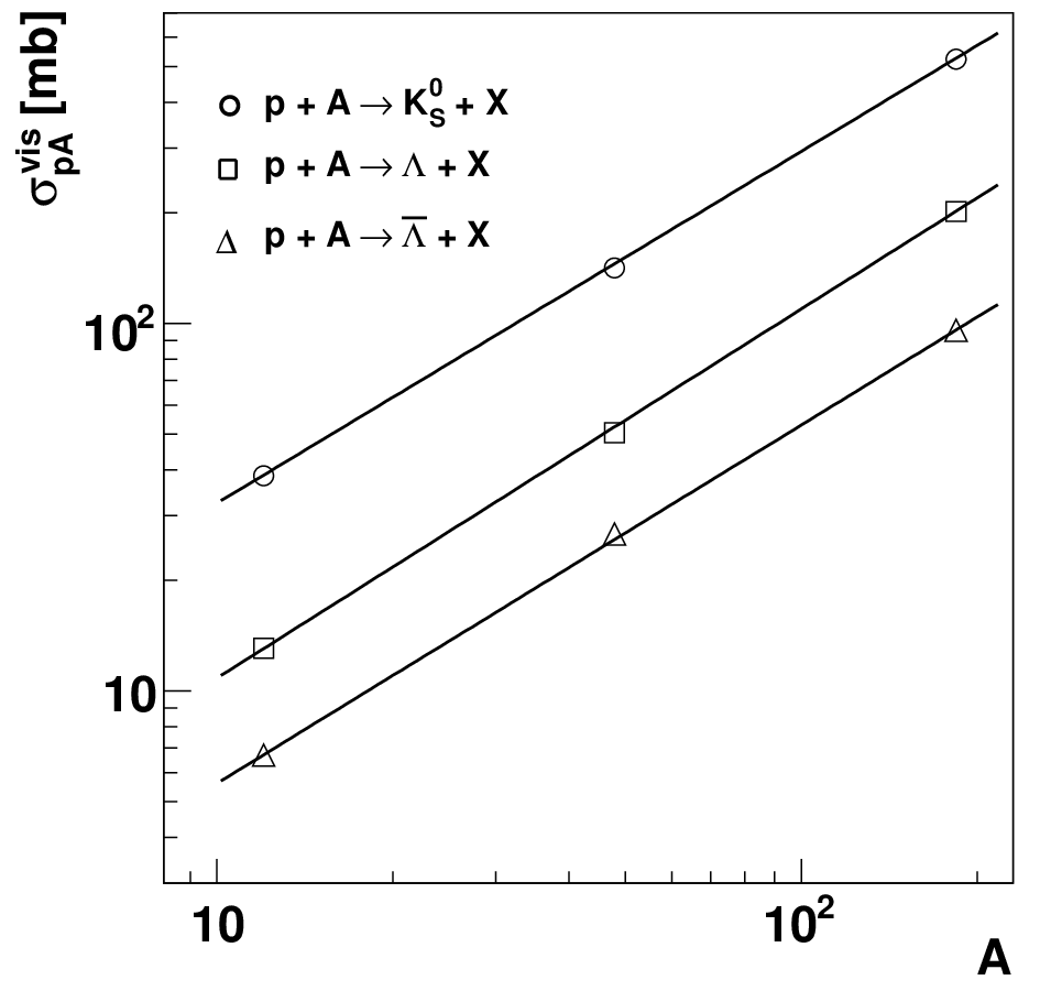
The dependence of the measured cross sections on the atomic mass of the target material (A) can be described by a power-law:
| (4) |
where, in this case, characterizes the average atomic mass number dependence of the visible cross section. The systematic uncertainties on the individual cross section measurements are highly correlated between the target materials, therefore the least-squares likelihood function used to extract and uses the full error matrix of the measurements. The visible cross sections, together with the fitted curves are shown in Fig. 4. The fit results and s are given in Table 4.
The dependences of on and on are shown on Fig. 5. The solid lines are from straight-line fits whose parameters are given in Table 4 and the dashed lines are the EPOS predictions. The Cronin effect manifests itself as an increase of with increasing . The EPOS curves reproduce the dependence rather well except for the first bins where EPOS underestimates . Since the main contributions to the cross sections are at low , the EPOS predictions lie well under the data points in the vs. plots although the trends with is the same within errors.
The total cross sections (also given in Table 4) are found be dividing the visible cross sections by the fraction of the total cross section in the visible region. This fraction was estimated using an average of EPOS results for the fractions of all s produced in proton-proton and proton-neutron interactions in the measured interval (34.7%, 17.5% and 35.4% for , and , respectively). The alternative of separately correcting each proton-nucleus cross section before extrapolation to was rejected since it relies more heavily on the Monte Carlo.
5.3 Particle ratios


The ratio of the cross section to that of the is plotted in Fig. 6 as functions of and for the three targets. For Fig. 6a, the data have been summed over the full measured range, and for Fig. 6b, over the full range. The EPOS calculations are also shown. The PYTHIA result indicated in Fig. 6b, is well above the data. The PYTHIA result vs. is well above the upper plot boundary in Fig. 6a, starting at at , and increasing smoothly to at . The EPOS result is in reasonable agreement with the data in Fig. 6a, where it is also seen to reproduce the A-dependence fairly well, despite the fact that the EPOS calculation of average is well below the data for both and (see Figs. 5b and 5c). As illustrated in Fig. 6b, the EPOS curve is also in reasonable agreement with the data over most of the range but the data shows a tendency to decrease with while EPOS suggests a flat dependence.
The ratio of to cross sections is shown in Fig. 7 for the three target materials. The STAR measurements [26] in interactions at and UA1 [25] in interactions at are also shown. The ratio shows no appreciable dependence on center-of-mass energy, atomic number or the type of colliding particles over the measured range. The EPOS results agree well with the data at low but tend to underestimate the data at higher . Nonetheless, as indicated in the figure, the EPOS calculation lies far closer to the data than the PYTHIA result over the full measured range.
5.4 Comparison with existing data
Only two experiments [21, 23] have measured production at a similar energy and in kinematic ranges which overlap with the present measurement. The first of these measurements, by Büsser et al., gives the average invariant cross section as a function of of three separate measurements at , , and (an average energy of ) in proton-proton collisions and in a center-of-mass rapidity () interval of about 2 units centered at 0 and for larger than 1.2 GeV/c() and 0.8 GeV/c ( and ). The measurements are shown in Fig. 8. The second report, by Drijard et al. [23] gives invariant cross sections for , , and over a wide range in rapidity and in proton-proton collisions at GeV. The relevant points are also shown in Fig. 8. The HERA-B measurements are indicated in Fig. 8 by curves which are derived from the parameterization given by (Eq. 3). The fit parameters are fixed to those of the carbon target (Table 2) and the resulting values are extrapolated to assuming the straight line fits to the vs. points shown in Fig. 5.
While the cross sections of [21] are in rather good agreement with the HERA-B results, the HERA-B and measurements are somewhat higher. Büsser et al. also extrapolate their measurements to and report mb () and mb (). The corresponding numbers for the present measurement, mb () and ( mb () are nearly a factor of two higher. As shown in Fig. 8, the measurements of [50] are also about a factor of two higher than the present measurement. This is, at least in part, explained by the substantially higher center-of-mass energy of the Drijard et al. measurements, however possible problems with the measurements reported in [23] have been noted [30] elsewhere.
Finally, in Fig. 9, we show the HERA-B results together with previously published values of the total proton-nucleon cross section as a function of squared CM energy (). The HERA-B results fit with the general trend of the data. Two notable exceptions are the two points at and indicated by squares ()and triangles () from Erhan et al. [22] for and production. We note however that these points depend sensitively on the extrapolations of Büsser et al.[21] and that a multiplicative factor of two is missing from the transformation given in [22] of the Büsser et al. points from to [51]. If our own measurements are substituted for the Büsser et al. extrapolations, we estimate that the total cross section values of Erhan et al. would increase by about a factor of two and a more satisfactory agreement among the different measurements would result, as indicated by the recalculated points in the figure.


6 Systematic uncertainties and checks
| signal counting | |||
|---|---|---|---|
| cut variation | |||
| tracking efficiency | |||
| branching ratio | |||
| MC model | |||
| total (w/o luminosity) | |||
| C | Ti | W | |
| luminosity (tot) | |||
| luminosity (uncorrelated) | |||
The following possible sources of systematic uncertainty have been considered:
- •
A bin-based method is used for estimating the number of produced candidates. An alternative fit-based method in which the invariant mass distributions are fit to a double Gaussian for the signal and a first-order Legendre polynomial for the background results in changes to the cross sections of 3.2% for , 3.3% for and 4.5% for .
- •
From varying the most powerful cut, namely the cut on , within reasonable limits, we estimate a systematic uncertainty of about 3.9% for , 5.2% for and 0.4% for mesons.
- •
The efficiencies for reconstruction of track segments in the VDS and in the OTR were measured independently by exploiting decays [49] of the . One of the two decay pions was reconstructed using RICH and ECAL information instead of either the OTR hits or the VDS hits and a search was made among the reconstructed tracks for a match. Based on a comparison of this method applied to data and to Monte Carlo, a systematic uncertainty on track reconstruction and matching efficiency of 1.5 per track is estimated.
- •
The influence of the track multiplicity on the reconstruction efficiency is found to give a negligible contribution to the systematic uncertainty.
- •
The systematic uncertainties on the branching ratios [38] are 0.05% for and 0.5% for and decays, respectively.
- •
The total systematic uncertainties due to the luminosity calculations [39] are 5.0%, 5.2% and 4.2% for carbon, titanium and tungsten targets, respectively. The uncertainties are correlated between target materials with correlation coefficients varying between 0.90 and 0.92. For the A-dependence and pN cross section results, these uncertainties and their correlations are taken into account.
- •
A check for a possible left-right bias in the spectrometer acceptance was made by deriving the visible cross section with subsets of the data with opposite signs of decay asymmetry (, where and are the components of momentum along the beam direction of and , respectively). The maximum difference between the values of cross sections for the negative and positive asymmetry samples is .
- •
The fact that the efficiency correction was done on a grid of and bins considerably reduces the dependence of the correction on the shape of the kinematic distributions produced by the MC compared to separate one-dimensional corrections. The remaining uncertainty was studied by varying - and -dependent weighting factors applied to the MC events. The difference between the average efficiency computed with a weight of unity and a weighting map which forces FRITIOF-generated distributions to conform to the corrected data is taken as the systematic uncertainty on the MC production model. The numbers are given in Table 5.
- •
In [52], we reported evidence for a positive polarization of ’s relative to the normal to the production plane in the visible region. Nonetheless the acceptance calculations done for the present measurement assume unpolarized production of ’s. It is however also shown in [53] that the acceptance is insensitive to polarization effects.
- •
The proper lifetimes of , and extracted from the data sample are cm, cm and cm, respectively (statistical errors only). The and lifetimes are within of the PDG values [38] while the measured lifetime is higher than the PDG value. The level of agreement is thus acceptable.
The systematic uncertainty estimates resulting from these considerations are collected in Table 5. The systematic uncertainties on the differential cross section measurements are quadratic sums of luminosity-dependent and -type dependent terms and are largely correlated over the measured range and constant to within about 20%. Since the uncertainties are for the most part correlated and constant, they appear as uncertainties in the overall scale depending only on target material and type and are quoted in Tables 6, 7 and 8.
7 Summary
We have studied the production cross sections for , , and in the central region () in proton interactions on nuclear targets (carbon, titanium and tungsten) at a center-of-mass energy of . The main results, the doubly differential cross sections are presented in Tables 6, 7, and 8. Several derived quantities: particle ratios, the -dependence parameter , and the total production cross sections are presented and discussed. The results are compared to PYTHIA and EPOS calculations. For the most part, the EPOS calculations agree with the data at the 20% level. PYTHIA is not designed to handle proton nucleus interactions and, as expected, produces distributions which are steeper than the data. PYTHIA also fails to describe the ratio of to , and, as previously pointed out in [26], the ratio of to . The failure cannot be attributed to A-dependence. The results are also compared to existing measurements and possible reasons for some discrepancies are discussed.
Acknowledgments
We express our gratitude to the DESY laboratory for their strong support in the installation of running of the experiment and the subsequent data analysis. We are also indebted to the DESY accelerator group for their continuous efforts to provide the best possible beam conditions. The HERA-B experiment would not have been possible without the enormous effort and commitment of our technical and administrative staff. It is a pleasure to thank all of them. We thank Klaus Werner for providing EPOS predictions and also for making the EPOS code available to us.
| (scale uncertainty: ) | |||||||
| - – - | - – - | - – - | - – - | - – - | - – | sum | |
| sum | |||||||
| (scale uncertainty: ) | |||||||
| - – - | - – - | - – - | - – - | - – - | - – | sum | |
| sum | |||||||
| (scale uncertainty: ) | |||||||
| - – - | - – - | - – - | - – - | - – - | - – | sum | |
| sum | |||||||
| (scale uncertainty: ) | |||||||
| - – - | - – - | - – - | - – - | - – - | - – | sum | |
| sum | |||||||
| (scale uncertainty: ) | |||||||
| - – - | - – - | - – - | - – - | - – - | - – | sum | |
| sum | |||||||
| (scale uncertainty: ) | |||||||
| - – - | - – - | - – - | - – - | - – - | - – | sum | |
| sum | |||||||
| (scale uncertainty: ) | |||||||
| - – - | - – - | - – - | - – - | - – - | - – | sum | |
| sum | |||||||
| (scale uncertainty: ) | |||||||
| - – - | - – - | - – - | - – - | - – - | - – | sum | |
| sum | |||||||
| (scale uncertainty: ) | |||||||
| - – - | - – - | - – - | - – - | - – - | - – | sum | |
| sum | |||||||
References
- [1] N. N. Biswas et al., Nucl. Phys. B 167, 41 (1980)
- [2] S. Mikocki et al., Phys. Rev. D 34, 42 (1986)
- [3] D. Ljung et al., Phys. Rev. 15, 3163 (1977)
- [4] D. Bogert et al., Phys. Rev. D 16, 2098 (1977)
- [5] R. T. Edwards et al., Phys.Rev. D 18, 76 (1978)
- [6] B. Y. Oh et al., Nucl. Phys. B 49, 13 (1972)
- [7] V. Blobel et al., Nucl. Phys. B 69, 454 (1974)
- [8] K. Jaeger et al., Phys. Rev. D 11, 1756 (1975)
- [9] H. Bøggild et al., Nucl. Phys. B 57, 77 (1973)
- [10] M. Alston-Garnjost et al., Phys. Rev. Lett. 35, 142 (1975)
- [11] J. W. Chapman et al., Phys. Lett. B 47, 465 (1973)
- [12] K. Jaeger et al., Phys. Rev. D 11, 2405 (1975)
- [13] A. Sheng et al., Phys. Rev. D 11, 1733 (1975)
- [14] K. Heller et al., Phys. Rev. D 16, 2737 (1977)
- [15] P. Skubic et al., Phys. Rev. D 18, 3115 (1978)
- [16] F. T. Dao et al., Phys. Rev. Lett. 30, 1151 (1973)
- [17] M. Asai et al., Z. Phys. C27, 11 (1985)
- [18] H. Kichimi et al., Phys. Rev. D 20, 37 (1979)
- [19]
A. Aleev et al., Yad. Fiz. 44 661, (1986);
Sov. J. Nucl. Phys. 44(3) 429, (1986) - [20] M. I. Adamovich et al., Eur. J. Phys. C 26, 357 (2003)
- [21] F. W. Büsser et al., Phys. Lett. B 61, 309 (1976)
- [22] S. Erhan et al., Phys. Lett. B 85, 447 (1979)
- [23] D. Drijard et al., Z. Phys. C 9, 293 (1981)
- [24] D. Drijard et al., Z. Phys. C 12, 217 (1982)
- [25] G. Bocquet et al., Phys. Lett. B 366, 441 (1996)
- [26] B.I. Adelev et al., Phys. Rev. C 75, 064901 (2007)
- [27] H. Jiang and X. Cai, Acta Phys. Hung. A 25, 313 (2006)
- [28] T. Sjostrand et al., Comp. Phys. Commun. 135, 238 (2001)
- [29] K. Werner et al., Phys. Rev. C 74, 044902 (2006)
- [30] I. Abt et al., Eur.Phys.J. C 29, 181 (2003)
- [31] E Hartouni. et al., HERA-B Design Report, DESY-PRC 95/01, (1995)
- [32] K. Ehret et al., Nucl Instr. Meth. A 446, 190 (2000)
- [33] C. Bauer et al., Nucl. Instr. Meth. A 501, 39 (2003)
- [34] H. Albrecht et al., Nucl. Instr. Meth. A 555, 319 (2005); H. Albrecht et al., Nucl. Instr. Meth. A 541, 610 (2005)
- [35] I. Ariño et al., Nucl. Instr. Meth. A 516, 445 (2004)
- [36] G. Avoni et al., Nucl. Instr. Meth A 580, 1209 (2007)
- [37] V. Eiges et al., Nucl. Instr. Meth A 461, 104 (2001)
- [38] C. Amsler et al., Phys. Lett. B 667, 1 (2008)
- [39] I. Abt et al., Nucl. Instr. Meth. A 582, 401 (2007)
- [40] I. Abt et al., Nucl. Instr. Meth. A 490, 546 (2002)
- [41] J. Podolansky and R. Armenteros, Fhil. Mag. 45, 13 (1954)
- [42] H. Pi, Comp. Phys. Comm. 71, 173 (1992)
- [43] R. Brun et al., GEANT3, CERN-DD-EE-84-1 (1987)
- [44] S. Brodsky and J. Gunion, Phys. Rev. D 17, 848, (1978)
- [45] G.W. van Apeldoorn et al., Nucl. Phys. B 91, 1 (1975)
- [46] M. Bardadin-Otwinowska et al., Phys Lett 21, 351 (1966)
- [47] J. Cronin et al., Phys. Rev. Lett. 38, 670 (1977)
- [48] W.M. Geist, Nucl. Phys. A 525, 149 (1991)
- [49] R. Pernack, PhD thesis, University of Rostock (2004)
- [50] HEPData DB, Durham, http://durpdg.dur.ac.uk/cgi-hepdata/hepreac/851590.
- [51] S. Erhan, Priv. Comm.
- [52] I. Abt et al., Phys. Lett. B 638, 415, 2006
- [53] E. Klinkby, Masters thesis, University of Copenhagen (2004).