Gauge Coupling Unification in F-theory GUT Models

The unification of the three gauge couplings of the strong and electroweak interactions at a scale $M_{X}=2.1\cdot 10^{16}\,$GeV in the minimal supersymmetric Standard Model (MSSM) is the strongest argument for the existence of a unifying grand unification at this high scale [1, 2, 3, 4]. The minimal simple gauge groups containing $SU(3)_{c}\times SU(2)_{w}\times U(1)_{Y}$ are $SU(5)$ and $SO(10)$. Besides the MSSM particles, these contain extra ones which have to receive a mass in the process of breaking the GUT gauge group. For a Georgi-Glashow $SU(5)$ GUT theory [5], there exist in particular the $X$ and $Y$ gauge bosons and in addition a vector-like pair of Higgs triplets $({\bf 3},{\bf 1})_{-{2\over 3}}+({\bf\overline{3}},{\bf 1})_{{2\over 3}}$ which combine with the weak Higgs doublet into the ${\bf 5}_{H}+{\bf\overline{5}}_{H}$ representation.

Combining the idea of a unification of gauge couplings with the unification of the gravitational interaction seems to be quite natural, as the GUT scale and Planck-scale $M_{pl}=2.4\cdot 10^{18}\,$GeV are not so far apart. Concrete examples for such a unification naturally arise from String Theory, where a compactification of for instance the $E_{8}\times E_{8}$ ten-dimensional heterotic string on a Calabi-Yau threefold ${\cal X}$ can lead to a four-dimensional effective field theory with ${\cal N}=1$ supersymmetry and gauge group $SU(5)$ or $SO(10)$. Since in most these string models there does not exist a light adjoint Higgs field, one has to implement an alternative mechanism by which the GUT gauge group is broken. In most cases this is done by turning on discrete Wilson lines supported on homologically non-trivial 1-cycles in the internal compact manifold.

Very recently, in the context of F-theory resp. Type IIB orientifold compactifications a different possibility has been made very concrete [6, 7]. Here the $SU(5)$ gauge group is supported on a stack of $D7$ branes wrapping a surface in the internal Calabi-Yau manifold ${\cal X}$. The three generations of chiral matter in the ${\bf 10}+{\bf\overline{5}}$ representation are localised on curves where the GUT brane intersects other branes. The same happens for the Higgs field ${\bf 5}_{H}+{\bf\overline{5}}_{H}$ which is also localised on such a curve. The GUT surface is chosen to be rigid, i.e. it is a del-Pezzo surface, so that there are no candidate $SU(5)$ adjoint Higgs fields. Moreover, a del-Pezzo surface does not admit any discrete Wilson line.

Similar to earlier considerations for the heterotic string [8, 9, 10], this leaves a third possibility to break the $SU(5)$ gauge group [11]. One can turn on an internal gauge flux $\overline{f}_{Y}$ with values in the $U(1)_{Y}$. One can describe this flux as a connection on some line bundle ${\cal L}_{Y}$, whose structure group breaks the $SU(5)$ to the SM gauge group. Usually, this would lead to Stückelberg masses for the four-dimensional hypercharge gauge field. However, if the $U(1)_{Y}$ flux is localised on a non-trivial two-cycle in the del-Pezzo, which is trivial when considered as a two-cycle in Calabi-Yau, the mass mixing with the axions can be avoided and the final gauge group is indeed $SU(3)_{c}\times SU(2)_{w}\times U(1)_{Y}$ [12]. We refer the reader to [6, 7, 11, 13, 14] for more details on such local F-theory models or to [15, 16] for the realisation on compact Type IIB orientifolds. A couple of phenomenological features of such models, like Yukawa textures [17, 18] and supersymmetry breaking [19], have been investigated recently.

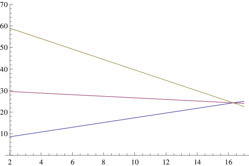
It is the aim of this letter to analyse the important issue of gauge coupling unification for such F-theory/IIB orientifold $SU(5)$ GUT models in more detail. Employing the formalism and notation put forward in [16], all computations are carried out in the Type IIB orientifold framework though they should carry over mutatis mutandis to the more general F-theory framework. The main new issue here is the presence of the $U(1)_{Y}$ flux, which at first sight causes a serious problem, in that it splits the values of the three MSSM gauge couplings at the string resp. unification scale. This might spoil the beautiful unification of these couplings shown in figure 1.

Let us assume that in either a local or a global model we have identified a del-Pezzo surface $D_{a}={\rm dP}_{r}$ on which we can wrap five D7-branes supporting a $U(5)$ gauge group. This surface is embedded into the Calabi-Yau as $\iota:D_{a}\to{\cal X}$. As shown in [16], via the Freed-Witten gauge flux quantisation condition, the fact that the del-Pezzo is non-Spin implies that these D7-branes must support a non-trivial line bundle ${\cal L}_{a}$. In the following we will choose this line bundle to come from a restriction of a line bundle on ${\cal X}$, i.e. ${\cal L}_{a}=\iota^{*}(L_{a})$.

The matter fields ${\bf 10}+{\bf\overline{5}}$ result from intersections of this $SU(5)$ brane with its orientifold image respectively a second single brane wrapping a divisor $D_{b}$ which supports a line bundle ${\cal L}_{b}$. In F-theory these matter fields are described as enhancements of the $SU(5)$ degeneration of the elliptic fiber of the fourfold to $SO(10)$ resp. $SU(6)$ along certain matter curves.

Now, one breaks the $SU(5)$ GUT theory by turning on a non-trivial $U(1)_{Y}$ flux ${\cal L}_{Y}$ supported on a two-cycle on the del-Pezzo surface which is however trivial in the Calabi-Yau, i.e. $\iota_{*}({\cal L}_{Y})=0$. Clearly, if the breaking of the $SU(5)$ is such that below the breaking scale one has precisely the MSSM matter, the running of the gauge couplings is such that at the one-loop level they unify at $M_{X}=2.1\cdot 10^{16}$GeV. The most natural scenario is that one identifies the GUT scale with the string scale.

Let us consider the tree-level gauge couplings at the string scale. The $SU(5)$ gauge kinetic function $f_{SU(5)}={4\pi\over g^{2}_{X}}+i\Theta$ is simply given by

where $g_{s}=e^{\varphi}$ denotes the string coupling constant and ${\rm Vol}(D_{a})={1\over 2}\int_{D_{a}}J\wedge J$ is the volume of the del-Pezzo surface $D_{a}$. However, the presence of the line bundles ${\cal L}_{a}$, ${\cal L}_{Y}$ generates subleading terms, which can be computed by dimensionally reducing the Chern-Simons action of the D7-brane wrapping the del-Pezzo surface $D_{a}$

In our case the overall flux $F$ has the following expansion

where $\lambda_{a}$ denote the eight traceless Gell-Man matrices and $\sigma_{i}$ the three traceless Pauli matrices. The capital letters $F_{G}$ denote the four-dimensional gauge fields and the small letters $\overline{f}$ the internal background fluxes. Now, inserting the expansion (3) into the Chern-Simons term (2) and extracting the $F\wedge F$ terms, we eventually find the three tree level gauge kinetic functions ¹¹ 1 These formulas differ from those derived in [13], which is due to the fact that here a different embedding, eq. (3), of the fractional line bundle ${\cal L}_{Y}$ into $U(5)$ has been used.

where we used ${\cal L}_{a}=\iota^{*}(L_{a})$ and $S=e^{-\varphi}+iC_{0}$ denotes the axio-dilaton field ²² 2 Twisting ${\cal L}_{a}=\iota^{*}(L_{a})$ by a “trivial” line bundle, i.e. ${\cal L}_{a}\to{\cal L}_{a}\otimes{\cal R}_{a}$ with $\iota_{*}({\cal R}_{a})=0$, eq. (4) changes such that $\int c^{2}_{1}({\cal L}_{Y})\to\int[\,c^{2}_{1}({\cal L}_{Y})+2\,c_{1}({\cal L}_{Y})\,c_{1}({\cal R}_{a})\,]$. Note that for $e_{Y}=c_{1}({\cal L}_{Y})$ and $e_{a}=c_{1}({\cal R}_{a})$ being roots of $E_{r}$ with $e_{Y}\cdot e_{a}=1$ this correction vanishes, thus leading to ordinary gauge coupling unification. . As usual in string theory, these couplings receive one-loop threshold corrections at order $M_{KK}\simeq O(M_{s})$ with $M_{KK}\simeq(1/{\rm Vol}(D_{a}))^{1\over 4}$, whose effect we ignore in the following at leading order.

For models without light exotics $({\bf 3},{\bf 2})_{5\over 3}+({\bf\overline{3}},{\bf 2})_{-{5\over 3}}$ originating from non-vanishing cohomology groups $H^{*}(D_{a},{\cal L}_{Y})$, we have to choose a line bundle ${\cal L}_{Y}$ supported on the $E_{r}$ sublattice of $H^{2}({\rm dP}_{r},\mathbb{Z})$ with $\int c^{2}_{1}({\cal L}_{Y})=-2$. In other words, $c_{1}({\cal L}_{Y})$ has to correspond to a root of $E_{r}$. We expect the masses of the lightest such states to be of order $M_{KK}$. Turning on this $SU(5)$ symmetry breaking flux, for finite $g_{s}$ the gauge couplings at the string scale $M_{s}$ do not unify any longer.

One might be tempted that this could explain the 4% deviation from MSSM gauge coupling unification at the 2-loop level [20]. However, for F-theory/IIB orientifold GUTs the order of the gauge couplings at the string scale is

which never occurs in [20] for any value of the scale $\mu$. Therefore, we seem to have a serious problem with gauge coupling unification in this class of GUT models.

As shown in the last section, at the string scale we find the relation

for $\Delta_{13}={3\over 5}{\alpha}^{-1}_{Y}-{\alpha}^{-1}_{s}$ and $\Delta_{23}={\alpha}^{-1}_{w}-{\alpha}^{-1}_{s}$. Intriguingly, this can also be written as

a relation which has already appeared for gauge couplings in more general Standard Model like four stack intersecting D6-brane models [22](see also [21]).

It is clear that, in order to have any chance that running up the low-energy couplings to the string scale, they satisfy relation (5) and (6), there must exist a new threshold in between. These new charged states must contribute to the running such that it creates a region for $\mu$, where the order of the gauge couplings is like in (5).

Recall that prior to GUT symmetry breaking, there were the Higgs fields ${\bf 5}_{H}+{\bf\overline{5}}_{H}$ and that the $U(1)_{Y}$ bundle was chosen such that the doublets remain massless and the triplets become massive, i.e.

Here $C$ denotes the curve $C\subset D_{a}$ supporting the Higgs fields and $K_{C}$ its canonical line bundle. In the case that the Higgs field is localised on a curve of genus one, the mass of the triplet is determined by a non-trivial Wilson line originating from the reduction of the line bundles on the genus one curve. These states have masses smaller than the Kaluza-Klein scale $M_{KK}$, which we assume to be (slightly) smaller than the order of the string scale. In [11] a second option was discussed, where the two Higgs fields are localised on different curves, so that via (8) the masses of the triplets come from pairings of ${\bf 3}_{H},{\bf\overline{3}}_{H}$ with other fields respectively. This allows to suppress dimension five proton decay operators.

Therefore, these colour triplets $({\bf 3},{\bf 1})_{-{2\over 3}}+({\bf\overline{3}},{\bf 1})_{{2\over 3}}$ are the distinguished natural candidates to change the running of the gauge couplings at a scale $M_{3\overline{3}}<M_{X}$ and we treat their mass scale as a parameter $1{\rm TeV}<M_{3\overline{3}}<M_{X}$ for the following analysis.

Above this new threshold the MSSM beta-function coefficients change according to

Choosing for instance $M_{3\overline{3}}=10^{15}\,$GeV, the running around the GUT scale changes as shown in figure 2.

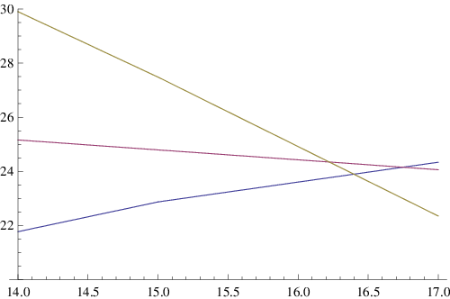
It is obvious that now there exist a region where the order of the gauge couplings is as in (5). Zooming in into this region we get figure 3.

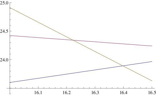
Now, in the region $16.2<\log_{10}(\mu)<16.4$ there must exist a point where precisely the relation (6) holds. Indeed, numerically we find that this happens at

which quite remarkably is the value of the usual GUT scale.

For analysing what happens around the GUT scale, we have to look more closely at the running of the gauge couplings between the threshold $M_{3\overline{3}}$ and the GUT scale. In fact, the running of the three gauge couplings at scales $\mu>M_{3\overline{3}}$ can be written as

Now requiring that the F-theory GUT relation (6) holds at $\mu=M_{X}=M_{s}$, leads to the simple relation

which is satisfied for any number of Higgs triplets and any threshold scale $M_{3\overline{3}}<M_{X}$.

Let us summarise the main observations made in this letter:

• •

  The breaking of the $SU(5)$ GUT via a non-trivial $U(1)_{Y}$ flux leads to a splitting of the three MSSM gauge couplings at the string/GUT scale

  $\displaystyle{1\over\alpha_{Y}(M_{s})}={1\over\alpha_{w}(M_{s})}+{2\over 3\alpha_{s}(M_{s})}\;,$

  (13)

  thus spoiling the usual gauge coupling unification.

• •

  If the Higgs triplet $({\bf 3},{\bf 1})_{-{2\over 3}}+({\bf\overline{3}},{\bf 1})_{{2\over 3}}$ is lighter than the GUT scale, this threshold changes the one-loop running of the gauge couplings such that they satisfy this F-theory GUT relation at $M_{X}$ independent of the value of the threshold scale.

• •

  In this case, from eq. (4), eq. (11) and $c_{1}({\cal L}_{Y})$ being a root of $E_{r}$, one can derive the following two additional relations with $\alpha_{X}^{-1}\simeq 24$

  $\displaystyle{1\over g_{s}}={1\over 2\pi}\log\left({M_{X}\over M_{3\overline{3}}}\right),\quad\ {M_{KK}\over M_{s}}\simeq\left({\alpha_{X}\over g_{s}}\right)^{1\over 4}$

  (14)

If the appearance of baryon number violating dim$=5$ operators $QQQL$ forces us to choose $M_{3\overline{3}}$ of the order of $M_{X}$, we get $g_{s}>1$, i.e. we are driven to the strong coupling regime, where F-theory is expected to be the appropriate description and where for $g_{s}\gg 1$ all corrections in (4) become negligible small. However, if there exists a mechanism to suppress these dangerous $QQQL$ operators, $M_{3\overline{3}}$ can be significantly smaller than $M_{X}$, while gauge coupling F-unification still holds. For $M_{3\overline{3}}<10^{13}\,$ GeV we even get $g_{s}<1$ with $M_{KK}=O(M_{X})$ ³³ 3 I thank D. Lüst and T. Weigand for helpful discussions..

Recall that in field theory GUTs one gets two relations among the gauge coupling constants at the GUT scale leading to one prediction for the couplings at the weak scale. In the F-theory case, one has instead only one direct relation among the gauge couplings (13) at the string scale, which already suffices to fix the GUT scale. In addition one finds one relation among the string parameters $g_{s}$ and $M_{3\overline{3}}$. If for a concrete string model one has prior knowledge that this relation holds, we also have one prediction among the gauge couplings at $M_{w}$. In the more general scheme with $g_{s}$ and $M_{3\overline{3}}$ treated as adjustable parameters F-theory is less predictive than a field theory GUT.

From the observation made in this letter one can draw two not unrelated conclusions. First, it shows the robustness of the $SU(5)$ gauge breaking mechanism by a $U(1)_{Y}$ flux. The shift in the string scale gauge couplings can be reconciled precisely by the running of the Higgs triplet below the string scale. Second, in all $SU(5)$ GUT models with the mass of the Higgs triplet significantly below the GUT scale, unification at $M_{X}=2.1\cdot 10^{16}\,$GeV requires the F-theory like split (7) in the GUT scale gauge couplings.

Finally, it is amusing that by writing equation (14) as $M_{3\overline{3}}=M_{s}\,\exp(-2\pi\Re(S))$ it looks, as if the Higgs triplet gets its dominant mass from a $D(-1)$-brane instanton.

Acknowledgements: I am very much indebted to Costas Bachas for reminding me to revisit the issue of gauge coupling unification in F-theory GUTs and to Dieter Lüst and Timo Weigand for very useful discussions. Moreover, I thank Michael Künkel and Sebastian Moster for further discussions.

References

- [1] J. R. Ellis, S. Kelley and D. V. Nanopoulos, Phys. Lett. B 249, 441 (1990).
- [2] U. Amaldi, W. de Boer and H. Fürstenau, Phys. Lett. B 260, 447 (1991).
- [3] C. Giunti, C. W. Kim and U. W. Lee, Mod. Phys. Lett. A 6 (1991) 1745.
- [4] P. Langacker and M. x. Luo, Phys. Rev. D 44 (1991) 817.
- [5] H. Georgi and S. L. Glashow, Phys. Rev. Lett. 32, 438 (1974).
- [6] R. Donagi and M. Wijnholt, arXiv:0802.2969 [hep-th].
- [7] C. Beasley, J. J. Heckman and C. Vafa, arXiv:0802.3391 [hep-th].
- [8] E. Witten, Nucl. Phys. B 268, 79 (1986).
- [9] R. Blumenhagen, S. Moster and T. Weigand, Nucl. Phys. B 751, 186 (2006) [arXiv:hep-th/0603015].
- [10] R. Tatar and T. Watari, arXiv:0806.0634 [hep-th].
- [11] C. Beasley, J. J. Heckman and C. Vafa, arXiv:0806.0102 [hep-th].
- [12] M. Buican, D. Malyshev, D. R. Morrison, H. Verlinde and M. Wijnholt, JHEP 0701, 107 (2007) [arXiv:hep-th/0610007].
- [13] R. Donagi and M. Wijnholt, arXiv:0808.2223 [hep-th].
- [14] J. Marsano, N. Saulina and S. Schäfer-Nameki, arXiv:0808.2450 [hep-th].
- [15] E. Plauschinn, arXiv:0811.2804 [hep-th].
- [16] R. Blumenhagen, V. Braun, T. W. Grimm and T. Weigand, arXiv:0811.2936 [hep-th].
- [17] A. Font and L. E. Ibanez, arXiv:0811.2157 [hep-th].
- [18] J. J. Heckman and C. Vafa, arXiv:0811.2417 [hep-th].
- [19] J. Marsano, N. Saulina and S. Schäfer-Nameki, arXiv:0808.1571 [hep-th].
- [20] M. Ibe and T. Watari, Phys. Rev. D 67, 114021 (2003) [arXiv:hep-ph/0303123].
- [21] L. E. Ibanez, C. Munoz and S. Rigolin, Nucl. Phys. B 553, 43 (1999) [arXiv:hep-ph/9812397].
- [22] R. Blumenhagen, D. Lüst and S. Stieberger, JHEP 0307, 036 (2003) [arXiv:hep-th/0305146].