Hodge decomposition in the homology of long knots

Victor Turchin Address: Kansas State University, USA. Email address: turchin@ksu.edu URL: http://www.math.ksu.edu/˜turchin/

Abstract.

The paper describes a natural splitting in the rational homology and homotopy of the spaces of long knots. This decomposition presumably arises from the cabling maps in the same way as a natural decomposition in the homology of loop spaces arises from power maps. The generating function for the Euler characteristics of the terms of this splitting is presented. Based on this generating function we show that both the homology and homotopy ranks of the spaces in question grow at least exponentially. Using natural graph-complexes we show that this splitting on the level of the bialgebra of chord diagrams is exactly the splitting defined earlier by Dr. Bar-Natan. In the Appendix we present tables of computer calculations of the Euler characteristics. These computations give a certain optimism that the Vassiliev invariants of order $>20$ can distinguish knots from their inverses.

Key words and phrases:

knot spaces, embedding calculus, Bousfield-Kan spectral sequence, graph-complexes, Hodge decomposition, Hochschild complexes, operads, bialgebra of chord diagrams, gamma function

1991 Mathematics Subject Classification

Primary: 57Q45; Secondary: 55P62, 57R40

Plan of the paper. Main results

The paper is divided into 3 parts. The first part is introductive. We describe there some general facts and constructions about the knot spaces we study. We also define there a convenient terminology for the sequel. The only new thing in this part is the definition of the Hodge decomposition in the rational homology and homotopy of knot spaces. In the second part we introduce natural graph-complexes computing the rational homology and homotopy of knot spaces together with their Hodge splitting. This construction generalizes an earlier construction of Bar-Natan that describes the primitives of the bialgebra of chord diagrams. To recall the latter bialgebra is intimately related to the Vassiliev knot invariants, which are also called invariants of finite type. The main result of this part is Theorem 8.2. We also formulate there Conjecture 12.1 that gives one more motivation for the study of the Hodge decomposition. It says that the Hodge decomposition of one-dimensional knots encodes information about the homology and homotopy of higher dimensional knots. Part 3 is more computational. Its main result is Theorem 13.1 that describes the generating function of the Euler characteristics of the terms of the Hodge splitting. Based on the formula for the generating function we show that the ranks of the rational homology and homotopy of the spaces of long knots grow at least exponentially, see Theorems 17.1, 17.2, 17.4.

Part I Introduction

1. Spaces of long knots modulo immersions

Denote by $Emb_{d}$ , $d\geq 3$ , the space of long knots, i.e. the space of smooth non-singular embeddings ${\mathbb{R}}^{1}\hookrightarrow{\mathbb{R}}^{d}$ coinciding with a fixed linear embedding $t\mapsto(t,0,0,\ldots,0)$ outside a compact subset of ${\mathbb{R}}^{1}$ . Similarly $Imm_{d}$ is the space of long immersions. The homotopy fiber of the inclusion $Emb_{d}\hookrightarrow Imm_{d}$ will be denoted by $\overline{Emb}_{d}$ . This space $\overline{Emb}_{d}$ of long knots modulo immersion and its rational homology and homotopy will be the object of our study. Its homology has a more natural interpretation then that of $Emb_{d}$ .¹¹ 1 The homology $H_{*}(\overline{Emb}_{d},{\mathbb{Q}})$ , $d\geq 4$ , is the Hochschild homology of the Poisson algebras operad [23, 37, 38]. On the other hand $\overline{Emb}_{d}$ is homotopy equivalent to the product [35, Proposition 5.17]:

\overline{Emb}_{d}\simeq Emb_{d}\times\Omega^{2}S^{d-1}.

So, there is no much difference the homology and homotopy of $\overline{Emb}_{d}$ or of $Emb_{d}$ is studied.

Proposition 1.1.

The spaces $\overline{Emb}_{d}$ , $d\geq 3$ , are acted on by the operad $C_{2}$ of little squares.

Sketch of the proof.

R. Budney constructed a model for the spaces $Emb_{d}^{framed}$ , $d\geq 3$ , of framed long knots that have a natural $C_{2}$ -action [7]. His construction can be easily generalized to the space $Imm_{d}^{framed}$ of framed long immersions. The inclusion $Emb_{d}^{framed}\hookrightarrow Imm_{d}^{framed}$ turns out to be a map of $C_{2}$ -algebras. But the homotopy fiber of this inclusion is homotopy equivalent to $\overline{Emb}_{d}$ , which implies the result. ∎

In case $d\geq 4$ , there is a different construction of such an action due to D. Sinha [35]. It is an open question whether these two $C_{2}$ -actions are equivalent.

Corollary 1.2.

For any field of coefficients ${\mathbb{K}}$ the homology $H_{*}(\overline{Emb}_{d},{\mathbb{K}})$ is a graded bicommutative bialgebra.

Corollary 1.3.

Since the spaces $\overline{Emb}_{d}$ , $d\geq 4$ , are connected, then for a field ${\mathbb{K}}$ of characteristics zero the homology $H_{*}(\overline{Emb}_{d},{\mathbb{K}})$ is a graded polynomial bialgebra generated by $\pi_{*}(\overline{Emb}_{d})\otimes{\mathbb{K}}$ .

2. Cosimplicial model for $\overline{Emb}_{d}$

For any $d\geq 4$ , D. Sinha defined a cosimplicial model ${C_{d}}^{\bullet}=\{{C_{d}}^{n}\,|\,n\geq 0\}$ , whose homotopy totalization is weakly homotopy equivalent to $\overline{Emb}_{d}$ [34]. The $n$ -th stage ${C_{d}}^{n}$ of this model is an appropriate compactification of the configuration space of $n$ distinct points labeled by $1,2,\ldots,n$ in $I\times{\mathbb{R}}^{d-1}=[0,1]\times{\mathbb{R}}^{d-1}$ . The space ${C_{d}}^{n}$ can also be viewed as the space of (bipointed) embeddings $\{0,1,\ldots,n,n+1\}\hookrightarrow I\times{\mathbb{R}}^{d-1}$ sending 0 to $(0,\bar{0})$ and $n+1$ to $(1,\bar{0})$ . The codegeneracy $s_{i}\colon{C_{d}}^{n}\to{C_{d}}^{n-1}$ , $i=1\ldots n$ , is the forgetting of the $i$ -th point in configuration, the coface $d_{i}\colon{C_{d}}^{n}\to{C_{d}}^{n+1}$ , $i=0\ldots n+1$ , is the doubling of the $i$ -th point in the direction of the vector $(1,\bar{0})$ .

The homology $\{H_{*}({C_{d}}^{n},{\mathbb{K}}),\,n\geq 0\}$ , and homotopy $\{\pi_{*}({C_{d}}^{n})\otimes{\mathbb{K}},\,n\geq 0\}$ form respectively a cosimplicial coalgebra that we will denote by ${A_{d}}^{\bullet}$ :

{A_{d}}^{\bullet}=\{{A_{d}}^{n},\,n\geq 0\}=\{H_{*}({C_{d}}^{n},{\mathbb{K}}),\,n\geq 0\},

and a cosimplicial Lie algebra

{L_{d}}^{\bullet}=\{{C_{d}}^{n},\,n\geq 0\}=\{\pi_{*}({C_{d}}^{n})\otimes{\mathbb{K}},\,n\geq 0\}.

We will usually assume that ${\mathbb{K}}={\mathbb{Q}}$ .

The cosimplicial model ${C_{d}}^{\bullet}$ for $\overline{Emb}_{d}$ defines the Bousfield-Kan homology and homotopy spectral sequences, whose first term in the homological case is

E^{1}_{-p,*}=H_{*}^{Norm}({C_{d}}^{p},{\mathbb{K}})=N{A_{d}}^{p},

and in the homotopy case:

{{\mathcal{E}}}^{1}_{-p,*}=\pi_{*}^{Norm}({C_{d}}^{p})\otimes{\mathbb{K}}=N{L_{d}}^{p}.

Where the normalized part $H_{*}^{Norm}({C_{d}}^{p},{\mathbb{K}})=N{A_{d}}^{p}$ , $\pi_{*}^{Norm}({C_{d}}^{n})\otimes{\mathbb{K}}=N{L_{d}}^{p}$ is the intersection of kernels of degeneracies: $\bigcap_{i=1}^{p}\ker s_{i*}$ .

Theorem 2.1 ([1, 22, 23]).

For a field ${\mathbb{K}}$ of characteristics zero and for $d\geq 4$ , both the homology and homotopy Bousfield-Kan spectral sequences associated with ${C_{d}}^{\bullet}$ collapse at the second term:

E^{2}_{*,*}=E^{\infty}_{*,*}=H_{*}(\overline{Emb}_{d},{\mathbb{K}}),\qquad{\mathcal{E}}^{2}_{*,*}={\mathcal{E}}^{\infty}_{*,*}=\pi_{*}(\overline{Emb}_{d})\otimes{\mathbb{K}}.

This theorem means that rationally the homology and homotopy of $\overline{Emb}_{d}$ are computed by the normalized complexes:

\Tot{A_{d}}^{\bullet}=\left(\oplus_{n\geq 0}N{A_{d}}^{n},d\right),\qquad\qquad\Tot{C_{d}}^{\bullet}=\left(\oplus_{n\geq 0}N{C_{d}}^{n},d\right),

where the differential $d$ is as usual the alternated sum of cofaces $d=\sum_{i=0}^{n+1}(-1)^{i}d_{i*}$ .

3. Hodge decomposition

As usual we assume that the main field of coefficients ${\mathbb{K}}$ is of characteristics zero. Gerstenhaber and Schak [16] defined the so called Hodge decomposition in the Hochschild (co)homology of commutative algebras with coefficients in a symmetric bimodule $M$ over $A$ .

(3.1)

HH_{*}(A,M)=\oplus_{i}HH_{*}^{(i)}(A,M),\qquad HH^{*}(A,M)=\oplus_{i}HH_{(i)}^{*}(A,M).

The construction of Gerstenhaber and Schak [16] used the $S_{n}$ -action on the components of Hochschild complexes:

(\oplus_{n\geq 0}M\otimes A^{\otimes n},\delta),\qquad(\oplus_{n\geq 0}Hom(A^{\otimes n},M),d).

They defined the families of orthogonal projectors $e_{n}^{(i)}\in{\mathbb{K}}[S_{n}]$ , $1\leq i\leq n$ if $n>0$ , and $i=0$ if $n=0$ , satisfying the following properties:

(3.2)

\bullet

e_{n}^{(i)}\cdot e_{n}^{(j)}=\delta_{ij}e_{n}^{(i)}

(they are orthogonal projectors);

\bullet

\sum_{i=0}^{n}e_{n}^{(i)}=1

(the family of projectors

e_{n}^{(i)}

i=0\ldots n

, is complete);

\bullet

\delta e_{n}^{(i)}=e_{n-1}^{(i)}\delta

de_{n}^{(i)}=e_{n+1}^{(i)}d

0=1\ldots n

In the above formula $e_{n}^{(i)}=0$ if $i$ is not in the range $1\ldots n$ (in case $n=0$ one has $e_{0}^{(i)}=0$ if $i\neq 0$ ).

By the last property the complexes ( ( 3.1 ) ) split into a direct sum of complexes with the $i$ -th complex being the image of the projection $e^{(i)}=\sum_{n=0}^{\infty}e_{n}^{(i)}$ . This splitting induces splitting in Hodge (co)homology which is called “Hodge decomposition”. Notice that the same construction works equally well in the differential graded setting [8, 40].

Later on J.-L. Loday gave a more general set up for this splitting [28]. He noticed that it takes place for any (co)simplicial complex that can be factored through the category $\Gamma$ (resp. $\Gamma^{op}$ ) of finite pointed sets. Recall that a simplicial (resp. cosimplicial) vector space is a functor from the category $\Delta^{op}$ (resp. $\Delta$ ) to the category of vector spaces:

X_{\bullet}\colon\Delta^{op}\longrightarrow Vect,\qquad X^{\bullet}\colon\Delta\longrightarrow Vect.

We will also consider cosimplicial dg-vector spaces. In that case the target category is $dg-Vect$ differential graded vector spaces. The objects of $\Delta^{op}$ are sets

[n]=\{0,1,\ldots,n+1\},\,\,n=0,1,2,\ldots

The morphisms are the bipointed ordered maps $[n]\to[m]$ preserving the linear order. By “bipointed” we mean maps sending 0 to 0, and $n+1$ to $m+1$ . The morphisms are generated by the so called face maps:

d_{i}\colon[n]\to[n-1],\quad i=0\ldots n,

d_{i}(j)=\begin{cases}j,&\text{if $j\leq i$;}\\ j-1,&\text{if $j>i$}\end{cases}

(the preimage $d_{i}^{-1}(i)$ has two points $i$ and $i+1$ ), and degeneracies:

s_{i}\colon[n]\to[n+1],\quad i=1\ldots n+1,

s_{i}(j)=\begin{cases}j,&\text{if $j<i$;}\\ j+1,&\text{if $j\geq i$}\end{cases}

(the preimage $d_{i}^{-1}(i)$ is empty).

The simplicial and cosimplicial complexes are defined as follows:

(3.3)

(\oplus_{n\geq 0}X_{n},\partial),\qquad(\oplus_{n\geq 0}X^{n},d),

where the differential $\partial$ (respectively $d$ ) is the alternated sum of (co)faces $d_{i}$ plus (in the differential graded case) the inner differential of each $X_{n}$ (respectively $X^{n}$ ).

It is usually convenient to consider the normalized complexes:

\Tot X_{\bullet}=(\oplus_{n\geq 0}NX_{n},\partial),\qquad\Tot X^{\bullet}=(\oplus_{n\geq 0}NX^{n},d),

which are quasi-isomorphic to the initial ones ( ( 3.3 ) ). The normalized part is defined as follows

NX_{n}=X_{n}\left/+_{i=1}^{n}\mathrm{Im}\,s_{i},\right.\qquad NX^{n}=\cap_{i=1}^{n}\mathrm{ker}\,s_{i}.

The category $\Gamma$ has objects

(3.4)

\underline{n}=\{*,1,2,\ldots,n\},\,\,n=0,1,2,\ldots

The morphisms $Mor_{\Gamma}(\underline{m},\underline{n})$ are the pointed maps $\underline{m}\to\underline{n}$ (we consider each set ( ( 3.4 ) ) to be pointed in $*$ ). One has a natural functor $\rho\colon\Delta^{op}\longrightarrow\Gamma$ induced by the set maps:

[n]\stackrel{{\scriptstyle\rho}}{{\longrightarrow}}{\underline{n}},

\rho(i)=\begin{cases}i,&1\leq i\leq n;\\ *,&\text{$i=0$ or $n+1$}.\end{cases}

By abuse of the language $\rho(d_{i})$ , $\rho(s_{i})$ will still be denoted by $d_{i}$ , $s_{i}$ and called faces and degeneracies respectively. The morphisms of $\Gamma$ are generated by faces, degeneracies, and also by the isomorphisms of each object $\underline{n}$ (that are given by the $S_{n}$ -group action).

Remark 3.1.

Let $\Gamma_{cycl}$ denote the subcategory of $\Gamma$ , whose objects are the same and morphisms are the pointed maps $\underline{m}\to\underline{n}$ preserving the cyclic order. It is easy to see, that $\Gamma_{cycl}$ is isomorphic to $\Delta^{op}$ via the functor $\rho$ :

\rho\colon\Delta^{op}\stackrel{{\scriptstyle\simeq}}{{\longrightarrow}}\Gamma_{cycl}.

J.-L. Loday noticed [28] that if a simplicial (resp. cosimplicial) differential graded vector space $X_{\bullet}$ (resp. $X^{\bullet}$ ) can be factored through the category $\Gamma$ (resp. $\Gamma^{op}$ ):

(3.5)

then each $X_{n}$ (resp. $X^{n}$ ) admits an $S_{n}$ -action, and moreover the projections $e_{n}^{(i)}\in{\mathbb{K}}[S_{n}]$ satisfy the properties ( ( 3.2 ) ), and therefore define the Hodge splitting

\Tot X_{\bullet}=\oplus_{i\geq 0}\Tot^{(i)}X_{\bullet},\qquad\Tot X^{\bullet}=\oplus_{i\geq 0}\Tot^{(i)}X^{\bullet}.

4. Operadic point of view. $\Sigma$ -cosimplicial spaces, and commutative $\Sigma$ -cosimplicial spaces

Notice that the Hodge splitting for Hochschild complexes was possible only for commutative algebras with coefficients in a symmetric bimodule. Only in this case the symmetric group action is “nicely” compatible with the differential which is built out of the product. In this section we define a natural formalism that generalizes this idea and will be helpful to detect $\Gamma$ and $\Gamma^{op}$ -modules.

Let ${\mathcal{O}}$ be any of the following three operads:

•

non- $\Sigma$ operad of associative algebras ${\mathcal{ASSOC}}=\{{\mathcal{ASSOC}}(n),\,n\geq 0\}$ whith ${\mathcal{ASSOC}}(n)={\mathbb{K}}$ for all $n$ .
•

operad of commutative algebras ${\mathcal{COMM}}=\{{\mathcal{COMM}}(n),\,n\geq 0\}$ with ${\mathcal{COMM}}(n)={\mathbb{K}}$ being the trivial representation of $S_{n}$ .
•

operad of associative algebras which will be also denoted by ${\mathcal{ASSOC}}=\{{\mathcal{ASSOC}}(n),\,n\geq 0\}$ , but in this $\Sigma$ -case ${\mathcal{ASSOC}}(n)={\mathbb{K}}[S_{n}]$ . To make a difference between non- $\Sigma$ et $\Sigma$ cases we will always specify which one is considered.

Definition 4.1.

$M=\{M(n),n\geq 0\}$ is a weak bimodule over the operad ${\mathcal{O}}$ if it is endowed with a series of composition maps:

(4.1)

\overline{\circ}_{i}\colon{\mathcal{O}}(n)\otimes M(k)\to M(n+k-1),\,\,i=1\ldots n,\text{ (left action)};

(4.2)

\underline{\circ}_{i}\colon M(k)\otimes{\mathcal{O}}(n)\to M(k+n-1),\,\,i=1\ldots k,\text{ (right action)},

satisfying natural associativity property, and (in the $\Sigma$ -case) compatibility with the $S_{n}$ -group action (in the $\Sigma$ -case we assume that $M(n)$ are $S_{n}$ -modules).²² 2 We say “weak” because the left action “is weak”. The usual left action is given by a series of maps ${\mathcal{O}}(k)\otimes\bigl(M(k_{1})\otimes M(k_{2})\otimes\ldots M(k_{n})\bigr)\to M(k_{1}+\ldots+k_{n})$ .

The result of composition $\overline{\circ}_{i}(o,m)$ , and $\underline{\circ}_{i}(m,o)$ , for $o\in{\mathcal{O}}(n)$ , and $m\in M(k)$ , will be denoted by $o\circ_{i}m$ , and $m\circ_{i}o$ .

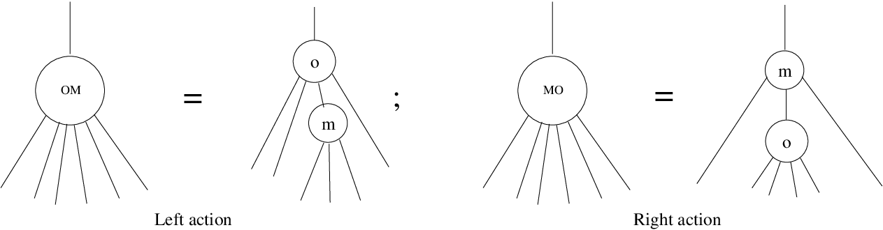
We will also adopt notation using formal variables. For example, $o\circ_{3}m$ from the above picture will be denoted as $o(x_{1},x_{2},m(x_{3},x_{4},x_{5}),x_{6})$ , and $m\circ_{2}o$ as $m(x_{1},o(x_{2},x_{3},x_{4},x_{5}),x_{6})$ .

Lemma 4.2.

The structure of a cosimplicial vector space is equivalent to the structure of a weak non- $\Sigma$ bimodule over (non- $\Sigma$ ) ${\mathcal{ASSOC}}$ .

Lemma 4.3.

The structure of a $\Gamma^{op}$ -module is equivalent to the structure of a weak bimodule over ${\mathcal{COMM}}$ .

The same is true in the differential graded case in which the acting operads ${\mathcal{ASSOC}}$ and ${\mathcal{COMM}}$ are considered with trivial differential.

Proof of Lemmas 4.2, 4.3.

Instead of giving a formal proof let us consider a few examples how cosimplicial and $\Gamma^{op}$ structure maps correspond to the composition operations ( ( 4.1 ) - ( 4.2 ) ). Let $M=\{M(n),\,n\geq 0\}$ be a non- $\Sigma$ weak bimodule over (non- $\Sigma$ ) ${\mathcal{ASSOC}}$ . Let us pick $m=6$ , $n=3$ , and some map $\alpha\in Mor_{\Delta^{op}}([6],[3])$ :

By Remark 3.1 this morphism corresponds to the following morphism in $Mor_{\Gamma_{cycl}}(\underline{6},\underline{3})$ .

We define the map $\alpha_{M}\colon M(3)\to M(6)$ using the compositions ( ( 4.1 ) ), ( ( 4.2 ) ):

Or equivalently

\alpha_{M}(m)(x_{1},x_{2},x_{3},x_{4},x_{5},x_{6})=x_{1}m(x_{2}x_{3},1,x_{4}x_{5}x_{6}).

By , , , , $\ldots$ in the above picture we represent respectively $1\in{\mathcal{ASSOC}}(0)$ , $x_{1}\in{\mathcal{ASSOC}}(1)$ , $x_{1}x_{2}\in{\mathcal{ASSOC}}(2)$ , $x_{1}x_{2}x_{3}\in{\mathcal{ASSOC}}(3)$ , $\ldots$ . The idea is to denote the output of $m$ and of $\alpha(m)$ by $*$ , and their inputs by $1,2,3,\ldots$ , and then to see how the output and inputs of $\alpha_{M}(m)$ are connected to the output and inputs of $M$ .

Similarly if $M$ is a weak bimodule over ${\mathcal{COMM}}$ , then any morphism $\alpha\colon\underline{m}\to\underline{n}$ defines a map $\alpha_{M}\colon M(n)\to M(m)$ . For example, the map $\alpha\colon\underline{4}\to\underline{2}$ :

defines a map $\alpha_{M}\colon M(2)\to M(4)$ constructed as follows:

Equivalently $\alpha_{M}(m)(x_{1},x_{2},x_{3},x_{4})=x_{1}x_{3}m(1,x_{2}x_{4})$ . ∎

We have seen that weak bimodules over ${\mathcal{COMM}}$ and weak non- $\Sigma$ bimodules over ${\mathcal{ASSOC}}$ have a very natural interpretation. Actually weak bimodules over ${\mathcal{ASSOC}}$ are also very common objects. As example the Hochschild complex of any (not necessarily symmetric) algebra $A$ with coefficients in its any bimodule has this structure. The category that encodes this structure is also well-known it is the category of finite pointed non-commutative sets [32].

The following definition is not standard, but will be convenient for the language of the paper.

Definition 4.4.

(a) A weak bimodule over ( $\Sigma$ operad) ${\mathcal{ASSOC}}$ will be called $\Sigma$ -cosimplicial space.

(b) A weak bimodule over ${\mathcal{COMM}}$ or equivalently $\Gamma^{op}$ -module will be called commutative $\Sigma$ -cosimplicial space.

Roughly speaking $\Sigma$ -cosimplicial spaces are cosimplicial spaces with $S_{n}$ action on each component, and commutative $\Sigma$ -cosimplicial spaces are $\Sigma$ -cosimplicial spaces for which this $S_{n}$ action is nicely compatible with the face maps.

4.1. In the category of topological spaces

Similar constructions (Lemmas 4.2-4.3, Definition 4.4) work well for any symmetric monoidal category with associative coproducts. Again abusing the notation ${\mathcal{COMM}}=\{{\mathcal{COMM}}(n),\,n\geq 0\}=\{*,\,n\geq 0\}$ will denote the topological commutative operad and ${\mathcal{ASSOC}}$ will denote both $\Sigma$ and non- $\Sigma$ associative operads:

	$\displaystyle\text{non-$\Sigma$ case: }{\mathcal{ASSOC}}=\{{\mathcal{ASSOC}}(n)=*,\,n\geq 0\}.$
	$\displaystyle\text{$\Sigma$ case: }{\mathcal{ASSOC}}=\{{\mathcal{ASSOC}}(n)=S_{n},\,n\geq 0\}.$

4.2. Subcomplex of alternative multiderivations

There is one important case when the Hochschild cohomology is easy to compute. This is when $A$ is a smooth algebra, and $M$ is its flat symmetric bimodule. In this case the cohomology $HH^{*}(A,M)$ is described by the space of alternative multiderivations.

Definition 4.5.

Let $Y^{\bullet}$ be a commutative $\Sigma$ -cosimplicial $dg$ -vector space.

(a) An element $y\in Y^{\bullet}$ is called alternative if for any $\sigma\in S_{n}$

(4.3)

y(x_{\sigma_{1}},x_{\sigma_{2}},\ldots,x_{\sigma_{n}})=(-1)^{|\sigma|}y(x_{1},x_{2},\ldots,x_{n}).

(b) An element $y\in Y^{n}$ is called a multiderivation if for any $i=1\ldots n$ one has

(4.4)

y(x_{1},\ldots,x_{i-1},x_{i}x_{i+1},x_{i+2},\ldots,x_{n+1})=\\ x_{i}y(x_{1},\ldots,\hat{x}_{i},\ldots,x_{n+1})+y(x_{1},\ldots,\hat{x}_{i+1},\ldots,x_{n+1})x_{i+1}.

Let $AM(Y^{n})$ denote the subspace of alternative multiderivations in $Y^{n}$ .

Lemma 4.6.

The space $AM(Y^{n})$ , $n\geq 0$ , is a subcomplex of $\Tot Y^{\bullet}$ .

Proof.

Let $y\in AM(Y^{n})$ . For any $1\leq i\leq n$ one has

s_{i}y=y(x_{1},\ldots,x_{i-1},1,x_{i},\ldots,x_{n-1})=y(x_{1},\ldots,x_{i-1},1\cdot 1,x_{i},\ldots,x_{n-1})=\\ 1\cdot y(x_{1},\ldots,x_{i-1},1,x_{i},\ldots,x_{n-1})+y(x_{1},\ldots,x_{i-1},1,x_{i},\ldots,x_{n-1})\cdot 1=2s_{i}y.

Therefore $s_{i}y=0$ .

On the other hand the external part of the differential, which is the alternative sum of cofaces $d_{i}$ , takes any multiderivation to zero, which can be checked by similar computations. One has also that the internal part of the differential preserves the alternative and multiderivation properties since it commutes with $\Gamma^{op}$ structure maps. ∎

The complex $\oplus_{n\geq 0}AM(Y^{n})$ will be also denoted by $AM(Y^{\bullet})$ . The following definition is inspired by the example from the beginning of the section.

Definition 4.7.

A commutative $\Sigma$ -cosimplicial $dg$ -vector space will be called smooth if the inclusion

AM(Y^{\bullet})\hookrightarrow\Tot Y^{\bullet}

is a quasi-isomorphism.³³ 3 This definition is a weaker version of [31, Definition 4.3] given by Pirashvili. [31, Theorem 4.6] implies that smooth $\Gamma$ -modules in the sense of Pirashvili are always smooth in our definition.

Remark 4.8.

For a smooth commutative $\Sigma$ -cosimplicial $dg$ -vectror space, the Hodge decomposition in the homology can be easily understood:

H_{*}^{(i)}(\Tot Y^{\bullet})=H_{*}(AM(Y^{i})).

This follows from the fact that $AM(Y^{i})$ lies in the image of $e_{i}^{(i)}=\frac{1}{i!}\sum_{\sigma\in S_{i}}(-1)^{|\sigma|}\sigma.$

5. Hodge decomposition in the homology and homotopy of long knots

Let $Top$ denote the category of topological spaces, and $hoTop$ denote the category with the same objects $Ob(hoTop)=Ob(Top)$ , but with the morphisms being the homotopy classes of maps. One has a forgetful functor:

(5.1)

Top\stackrel{{\scriptstyle h}}{{\longrightarrow}}hoTop.

Proposition 5.1.

The cosimplicial space ${C_{d}}^{\bullet}$ (see Section 2) has the property that $h\circ{C_{d}}^{\bullet}$ factors through $\Gamma^{op}$ :

(5.2)

or in other words ${C_{d}}^{\bullet}$ is a commutative $\Sigma$ -cosimplicial space in $hoTop$ .

Proof.

D. Sinha constructed another cosimplicial model for $\overline{Emb}_{d}$ , which is homotopy equivalent to the one that we briefly described in Section 2. The $n$ -th stage of this model is the $n$ -th component of some operad ${\mathcal{K}}_{d}$ which is homotopy equivalent to the operad of little $d$ -cubes. Using a natural inclusion

(5.3)

{\mathcal{ASSOC}}\hookrightarrow{\mathcal{K}}_{d},

${\mathcal{K}}_{d}$ becomes a cosimplicial space (being a bimodule over ${\mathcal{ASSOC}}$ , see Lemma 4.2). But ( ( 5.3 ) ) is a morphism of $\Sigma$ -operads. Therefore ${{\mathcal{K}}_{d}}^{\bullet}$ is a $\Sigma$ -cosimplicial space. But notice that all the components $K_{d}(n),$ $n\geq 0$ are connected, therefore in the category $hoTop$ the morphism ( ( 5.3 ) ) factors though ${\mathcal{COMM}}$ :

(5.4)

As a consequence in $hoTop$ the operad ${\mathcal{K}}_{d}$ is a weak bimodule over ${\mathcal{COMM}}$ , or equivalently is a commutative $\Sigma$ -cosimplicial space. ∎

Corollary 5.2.

Since the homology and homotopy functors factor through $hoTop$ , both the homology ${A_{d}}^{\bullet}=H_{*}({C_{d}}^{\bullet},{\mathbb{K}})$ and homotopy ${L_{d}}^{\bullet}=\pi_{*}({C_{d}}^{\bullet})\otimes{\mathbb{K}}$ of ${C_{d}}^{\bullet}$ are commutative $\Sigma$ -cosimplicial graded spaces.

There is another but similar way to see that ${A_{d}}^{\bullet}$ is a weak bimodule over ${\mathcal{COMM}}$ . The vector spaces $\{{A_{d}}^{n},\,n\geq 0\}$ form an operad, which is the homology operad of the little $d$ -cubes. By [10] it is the operad of $(d-1)$ -Poisson algebras: graded commutative algebras with a Lie bracket of degree $(d-1)$ compatible with the product:

[x_{1},x_{2}x_{3}]=[x_{1},x_{2}]x_{3}+(-1)^{|x_{2}|+(d-1)}x_{2}[x_{1},x_{3}].

This operad contains ${\mathcal{COMM}}$ and therefore is a weak bimodule over it.

Corollary-Definition 5.3.

The complexes $\Tot{A_{d}}^{\bullet}$ , $\Tot{L_{d}}^{\bullet}$ admit Hodge splitting

(5.5)

\Tot{A_{d}}^{\bullet}=\oplus_{i}\Tot^{(i)}{A_{d}}^{\bullet}.

(5.6)

\Tot{L_{d}}^{\bullet}=\oplus_{i}\Tot^{(i)}{L_{d}}^{\bullet}.

Since the above complexes compute the rational homology and homotopy of $\overline{Emb}_{d}$ , this gives the Hodge decomposition in its homology and homotopy:

(5.7)

H_{*}(\overline{Emb}_{d},{\mathbb{Q}})=\oplus_{i}H_{*}^{(i)}(\overline{Emb}_{d},{\mathbb{Q}}):=\oplus_{i}H_{*}(\Tot^{(i)}{A_{d}}^{\bullet}),

(5.8)

\pi_{*}(\overline{Emb}_{d})\otimes{\mathbb{Q}}=\oplus_{i}\pi_{*}^{(i)}(\overline{Emb}_{d},{\mathbb{Q}}):=\oplus_{i}H_{*}(\Tot^{(i)}{L_{d}}^{\bullet}).

6. Geometric interpretation of the Hodge decomposition. Cabling maps

Studying knot spaces is in many aspects similar to studying loop spaces. Recall that the real cohomology of the loop space $\Omega M$ of a 1-connected variety $M$ is naturally isomorphic to the Hochschild homology of the De Rham algebra $\Omega^{*}(M)$ (of differential forms on $M$ ) with trivial coefficients:

(6.1)

H^{*}(\Omega M,{\mathbb{R}})\simeq HH_{*}(\Omega^{*}(M),{\mathbb{R}}).

Similarly the cohomology of the free loop space $\Lambda M$ can be expressed as the Hochschild cohomology of $\Omega^{*}(M)$ with coefficients in itself:

(6.2)

H^{*}(\Lambda M,{\mathbb{R}})\simeq HH_{*}(\Omega^{*}(M),\Omega^{*}(M)).

The differential algebra $\Omega^{*}(M)$ is graded commutative, and both bimodules ${\mathbb{R}}$ , and $\Omega^{*}(M)$ are graded commutative over it. Hence it makes sense to consider the Hodge decomposition of ( ( 6.1 ) - ( 6.2 ) ). Let $\Phi_{n}$ denote the power maps

\Omega M\stackrel{{\scriptstyle\Phi_{n}}}{{\longrightarrow}}\Omega M,\qquad\Lambda M\stackrel{{\scriptstyle\Phi_{n}}}{{\longrightarrow}}\Lambda M.

induced by a degree $n$ map of a circle into itself $S^{1}\stackrel{{\scriptstyle n}}{{\longrightarrow}}S^{1}$ . It was shown in [8] that the Hodge decomposition in $HH_{*}(\Omega^{*}(M),{\mathbb{R}})$ (resp. $HH_{*}(\Omega^{*}(M),\Omega^{*}(M))$ ) corresponds via isomorphisms ( ( 6.1 ) ), ( ( 6.2 ) ) to the decomposition into eigenspaces of the power maps in cohomology:

H^{*}(\Omega M,{\mathbb{R}})\stackrel{{\scriptstyle\Phi_{n}^{*}}}{{\longrightarrow}}H^{*}(\Omega M,{\mathbb{R}}),\qquad H^{*}(\Lambda M,{\mathbb{R}})\stackrel{{\scriptstyle\Phi_{n}^{*}}}{{\longrightarrow}}H^{*}(\Lambda M,{\mathbb{R}}).

More precisely the $HH_{*}^{(i)}$ term is always the eigenspace of $\Phi_{n}^{*}$ with eigenvalue $n^{i}$ .

We believe that a similar assertion holds for the homotopy and homology of $\overline{Emb}_{d}$ . But instead of power maps one has to use cabling maps (abusing notation we will denote them similarly):

\Phi_{n}\colon\overline{Emb}_{d}\to\overline{Emb}_{d}.

The construction of $\Phi_{n}$ is similar to the proof of Proposition 1.1 and goes in 2 steps. First one constructs such maps for the spaces of long framed embeddings $Emb_{d}^{framed}$ , and long framed immersions $Imm_{d}^{framed}$ :

(6.3)

Below we show how to construct a 2-cabling of a framed long knot (framing is necessary to make the construction work on the level of spaces):

This construction works nicely if one uses Budney’s model for the space of framed long knots [7] (the space denoted by $EC(1,D^{d-1})$ ), and its analogue for the space of framed immersions. Since the diagram ( ( 6.3 ) ) commutes, one obtains the induced “cabling” map $\Phi_{n}$ on the homotopy fiber of the inclusion $Emb_{d}^{framed}\hookrightarrow Imm_{d}^{framed}$ . But this homotopy fiber is exactly $\overline{Emb}_{d}$ .

7. Relation between the Hodge decomposition in the homology and homotopy

Rational homotopy of $\overline{Emb}_{d}$ is isomorphic to the primitive part of the rational homology, see Corollary 1.2. By Theorem 2.1,

H_{*}(\overline{Emb}_{d},{\mathbb{Q}})=H_{*}(\Tot{A_{d}}^{\bullet}),\qquad\pi_{*}(\overline{Emb}_{d})\otimes{\mathbb{Q}}=H_{*}(\Tot{L_{d}}^{\bullet}).

Therefore the space of primitives of $H_{*}(\Tot{A_{d}}^{\bullet})$ is isomorphic to $H_{*}(\Tot{L_{d}}^{\bullet})$ :

(7.1)

Prim(H_{*}(\Tot{A_{d}}^{\bullet}))\simeq H_{*}(\Tot{L_{d}}^{\bullet})

A pure algebraic proof for this isomorphism is given in [22].

Proposition 7.1.

(i) The coproduct structure of $\Tot A^{\bullet}$ respects the Hodge degree:

\Delta\Tot^{(k)}{A_{d}}^{\bullet}\subset\bigoplus_{i=0}^{k}\Tot^{(i)}{A_{d}}^{\bullet}\otimes\Tot^{(k-i)}{A_{d}}^{\bullet}.

(ii) The isomorphism ( ( 7.1 ) ) respects the Hodge decomposition.

The above proposition means that the study of the Hodge decomposition in the homology or in the homotopy are two equivalent problems, since the homology $H_{*}(\Tot{A_{d}}^{\bullet})$ is a free graded cocommutative coalgebra over $Prim(H_{*}(\Tot{A_{d}}^{\bullet}))\simeq H_{*}(\Tot{L_{d}}^{\bullet})$ .

Proof.

The proof of (i) follows from the following lemma:

Lemma 7.2.

Let $B^{\bullet}$ and $C^{\bullet}$ be two commutative $\Sigma$ -cosimplicial spaces, then $B^{\bullet}\otimes C^{\bullet}$ is also a commutative $\Sigma$ -cosimplicial space and moreover the Eilenberg-Mac Lane map

\Tot(B^{\bullet}\otimes C^{\bullet})\to\Tot B^{\bullet}\otimes\Tot C^{\bullet}

respects the Hodge degree.

Proof.

This fact is well known. For example, one can see it from the geometric approach of F. Patras to describe Adams operations [29, 30] (see in particular Proposition 1.3 of [30] and the remark that follows.) ∎

To prove (i) we notice that the coproduct on $\Tot{A_{d}}^{\bullet}$ is obtained as a composition of two maps:

\Tot{A_{d}}^{\bullet}\stackrel{{\scriptstyle\Delta^{\bullet}}}{{\longrightarrow}}\Tot({A_{d}}^{\bullet}\otimes{A_{d}}^{\bullet})\stackrel{{\scriptstyle EM}}{{\longrightarrow}}\Tot{A_{d}}^{\bullet}\otimes\Tot{A_{d}}^{\bullet}.

The first map $\Delta^{\bullet}$ is induced by a degree-wise coproduct (in the homology of configuration spaces), which is a morphism of commutative $\Sigma$ -cosimplicial spaces. The second one respects the Hodge degree by Lemma 7.2.

(ii) Recall that the proof of ( ( 7.1 ) ) was given by the following sequence of quasi-isomorphisms:

(7.2)

where ${A_{d}}_{\bullet}$ is the simplicial graded commutative algebra dual to ${A_{d}}^{\bullet}$ (i.e. ${A_{d}}_{n}=H^{*}({C_{d}}^{n},{\mathbb{Q}})$ ), and ${L_{d}}_{\bullet}$ is the simplicial graded Lie coalgebra dual to ${L_{d}}^{\bullet}$ (i.e. ${L_{d}}_{n}=Mor(\pi_{*}({C_{d}}^{n}),{\mathbb{Q}})$ ). The algebra $\Tot{A_{d}}_{\bullet}$ is polynomial, $\Tot{A_{d}}_{\bullet}/(\Tot{A_{d}}_{\bullet})^{2}$ describes the quotient complex by all the non-generators. The homology of $\Tot{A_{d}}_{\bullet}/(\Tot{A_{d}}_{\bullet})^{2}$ is $Prim(H_{*}(\Tot{A_{d}}_{\bullet}))$ . The functor ${\mathcal{L}}(-)$ is the cobar construction that assigns to any commutative $dg$ -algebra a free $dg$ -Lie coalgebra. The first, and the second quasi-isomorphisms, $\alpha$ , and $EM_{\mathcal{L}}$ , respect the Hodge decomposition by Lemma 7.2. The last one is induced by a morphism of differential graded $\Gamma$ -modules and therefore respects the Hodge degree. ∎

Part II Graph-complexes

8. Bialgebra of chord diagrams. Generalizing a result of Bar-Natan

The bialgebra of chord diagrams is a well-known object in Low Dimensional Topology which encodes the so called Vassiliev invariants of knots. Bar-Natan has shown that this bialgebra is isomorphic to the bialgebra of unitrivalent graphs attached to a line modulo $STU$ , $IHX$ , and $AS$ relations [6]. Theorem 8.6 of [22] generalizes and also gives another proof of this result using graph-complexes. In this paper we will go a step further and will generalize the following result of Bar-Natan:

Theorem 8.1 (Bar-Natan [6]).

The space of primitive elements of the bialgebra of chord diagrams is isomorphic to the space of connected unitrivalent graphs (with at least one univalent vertex) modulo $IHX$ , and $AS$ relations.

The bialgebra of chord diagrams is naturally graded by complexity - number of chords. The complexity of a unitrivalent graph is the Betti number of the graph obtained by gluing together all univalent vertices, see Figure C.

From this theorem we see that the space of primitives has another grading which is the number of univalent vertices.

Theorem 8.2.

The homotopy $\pi_{*}(Emb_{d})\otimes{\mathbb{Q}}$ , resp. the homology $H_{*}(\overline{Emb}_{d},{\mathbb{Q}})$ is computed by the graph-complex $AM({P_{d}}^{\bullet})$ , resp. $AM({D_{d}}^{\bullet})$ (that we define below) of connected, resp. possibly disconnected or empty uni- $\geq 3$ -valent graphs. Moreover via this isomorphism the complexity grading is the first Betti number of the graph obtained by gluing together all the univalent vertices, and the Hodge degree is the number of univalent vertices.

This theorem is proved in Section 10.

Below we describe explicitly the complexes $AM({P_{d}}^{\bullet})$ , $AM({D_{d}}^{\bullet})$ .

8.1. Definition of $AM({P_{d}}^{\bullet})$ , $AM({D_{d}}^{\bullet})$

Let us first define the complex $AM({P_{d}}^{\bullet})$ . By a connected uni- $\geq 3$ -valent graph we mean a connected graph with a non-empty set of univalent vertices (which are called external) and some (possibly empty) set of vertices of valence at least 3 (those vertices are called external). The graphs are allowed to have both multiple edges and loops — edges connecting a vertex to itself:

Neither external, nor internal vertices are labeled. Two graphs are considered to be equivalent if there is a bijection between their sets of vertices and edges respecting the adjacency structure of the graphs.

The orientation set of a graph is the set of its external (univalent) vertices (those vertices are considered to have degree $-1$ ), its internal vertices (which are considered to have degree $-d$ ), and its edges (considered to have degree $(d-1)$ ). The total grading of a graph is the sum of gradings of its edges, and vertices. An orientation of a graph is an ordering of its orientation set together with fixing of orientation of each edge.

Definition 8.3.

The space of $AM({P_{d}}^{\bullet})$ is a graded vector space over ${\mathbb{K}}$ spanned by the above connected uni- $\geq 3$ -valent graphs modulo the orientation relations:

(1) If $\Gamma_{1}$ and $\Gamma_{2}$ differ only by an orientation of an edge, then

\Gamma_{1}=(-1)^{d}\Gamma_{2}.

(2) If $\Gamma_{1}$ and $\Gamma_{2}$ differ only by a permutation of an orientation set, then

\Gamma_{1}=\pm\Gamma_{2},

where the sign is a Koszul sign of permutation (taking into account the degrees of elements).

The differential in $AM({P_{d}}^{\bullet})$ is a sum of expansions of internal vertices, see example below.

Together with the main grading which is the sum of gradings of edges and vertices, we will consider two additional gradings. The first one, complexity, is defined as the first Betti number of the graph obtained by gluing all univalent vertices together, see Figure C. The second one, Hodge degree, is defined as the number of external vertices (we will later on see that indeed it corresponds to to the Hodge degree of some Hochschild complex). The differential in $AM({P_{d}}^{\bullet})$ preserves both the complexity and the Hodge degree, therefore the complex $AM({P_{d}}^{\bullet})$ splits into a direct sum of complexes:

AM({P_{d}}^{\bullet})=\oplus_{i,j}AM_{j}({P_{d}}^{i})

by complexity $j$ , and Hodge degree $i$ .

Remark 8.4.

Similar graph-complexes appear in the study of the homology of the outer spaces [12, 13, 19, 25]. The difference is that in our case the graphs have univalent vertices.

The second complex $AM({D_{d}}^{\bullet})$ can be defined as a free differential graded cocommutative coalgebra cogenerated by the complex $AM({P_{d}}^{\bullet})$ . This complex can also be viewed as a graph-complex of possibly empty or disconnected uni- $\geq 3$ -valent graphs, each connected component being from the space $AM({P_{d}}^{\bullet})$ .

The notation $AM(-)$ comes from “Alternative Multiderivations” (see Section 4.2). We will see in Section 10 that they are indeed isomorphic to the complexes of alternative multiderivations of the commutative $\Sigma$ -cosimplicial $dg$ -vector spaces ${P_{d}}^{\bullet}$ , and ${D_{d}}^{\bullet}$ .

9. Operadic graph-complexes

To recall the components of the cosimplicial space ${A_{d}}^{\bullet}=\{{A_{d}}^{n},\,n\geq 0\}=\{H_{*}({C_{d}}^{n}),\,n\geq 0\}$ form the operad of $(d-1)$ -Poisson algebras, that we also denote by $A_{d}$ .⁴⁴ 4 In [23, 37, 38] this operad was denoted by ${\mathcal{P}oiss}_{d-1}$ . We switched the notation for a convenience of presentation. In this section we define a series of graph-complexes $D_{d}=\{D_{d}(n),\,n\geq 0\}$ , that form an operad quasi-isomorphic to the operad $A_{d}$ . Moreover the quasi-isomorphism is given by a natural inclusion. The construction of $D_{d}$ takes roots in [21] and had a number of remakes [22, 24]. The difference of our construction is that we obtain an operad, and not a cooperad like in [21, 22, 24]. So our construction is dual to the previous ones. Another difference is that we also allow a little bit more admissible graphs: we permit graphs to have multiple edges (contrary to [21, 24], but similarly to [22]), and loops — edges connecting a vertex to itself (contrary to all previous versions). The $n$ -th component $D_{d}(n)$ is spanned by admissible graphs that have $n$ external vertices labeled by $1,2,\ldots,n$ , and some number of non-labeled internal vertices. The external vertices can be of any non-negative valence, the internal ones should be of valence at least 3. The only condition we put on graphs – each connected component should contain at least one external vertex (no pieces flying in air).

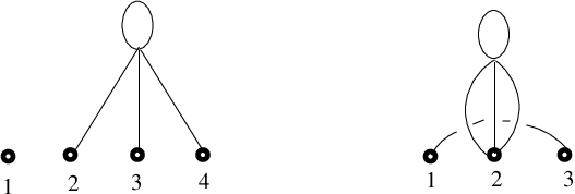
The orientation set of such a graph is the union of the set of internal vertices (those elements are considered to be of degree $-d$ ), and the set of edges (such elements are of degree $(d-1)$ ). Similarly to Section 8 we will say that a graph is oriented if one fixes orientation of all its edges, and an ordering of its orientation set. The space $D_{d}(n)$ is defined to be spanned by all oriented admissible graphs (with $n$ external vertices) modulo the orientation relations (1)-(2) similar to those of Definition 8.3.

Remark 9.1.

For even $d$ the orientation relations kill the graphs with multiple edges, and for odd $d$ — the graphs with loops.

The differential is the sum of expansions of vertices (being dual to to the sum of contractions of edges). It diminishes the total degree by 1. One should be a little bit careful with the external vertices. An expansion of an external vertex produces one external vertex (with the same label) and one internal one.

For the rule of signs see [24], or define any reasonable one by yourself.

The operadic structure defined by compositions

\circ_{i}\colon D_{d}(n)\otimes D_{d}(m)\to D_{d}(n+m-1)

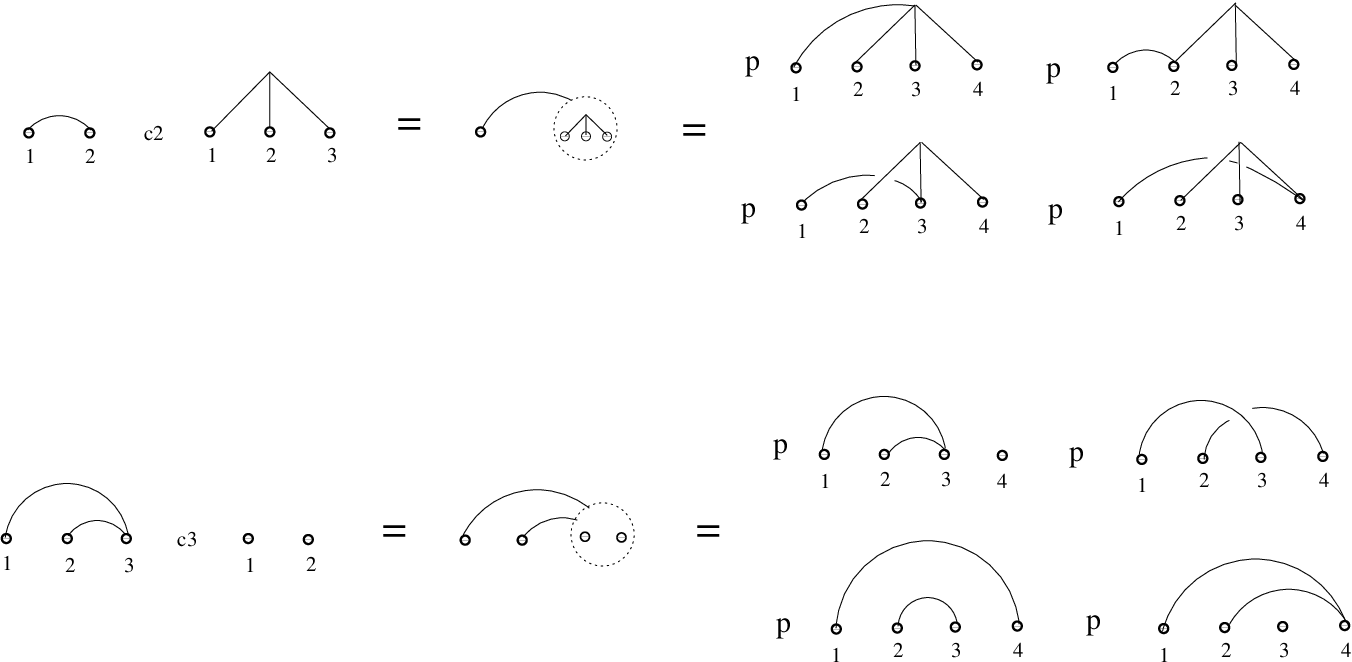
is dual to the cooperadic structure in [24]. If $\Gamma_{1}\in D_{d}(n)$ , $\Gamma_{2}\in D_{d}(m)$ two graphs, then $\Gamma_{1}\circ_{i}\Gamma_{2}$ is the sum of graphs obtained by making $\Gamma_{2}$ very small and inserting it in the $i$ -th external point of $\Gamma_{1}$ . The edges adjacent to the external vertex $i$ in $\Gamma_{1}$ become adjacent to one of the vertices of $\Gamma_{2}$ . The sum is taken by all such insertions, see Figure G.

Proposition 9.2.

The assignment

x_{1}x_{2}\mapsto\,\begin{picture}\put(2.0,5.0){\circle*{3.0}}\put(18.0,5.0){\circle*{3.0}}\put(0.0,-1.0){${}_{1}$}\put(16.0,-1.0){${}_{2}$}\end{picture}\,,\qquad[x_{1},x_{2}]\mapsto\,\begin{picture}\put(2.0,5.0){\circle*{3.0}}\put(18.0,5.0){\circle*{3.0}}\qbezier{}{2}{5}{10}{15}{18}{5}\put(0.0,-1.0){${}_{1}$}\put(16.0,-1.0){${}_{2}$}\end{picture}\,,

where $x_{1}x_{2},$ $[x_{1},x_{2}]\in A_{d}(2)$ are the product and the bracket of the operad $A_{d}$ of $(d-1)$ -Poisson algebras, defines an inclusion of operads

(9.1)

that turns out to be a quasi-isomorphism ( $A_{d}$ is considered to have a zero differential).

Proof.

This assertion is dual to [24, Theorem 9.1]. The graph-complexes used in [24] are slightly different, but the proof is the same. ∎

Notice that the operad $A_{d}$ contains the operad ${\mathcal{COMM}}$ . Therefore the inclusion ( ( 9.1 ) ) can be viewed as a morphism of weak bimodules over ${\mathcal{COMM}}$ . Denote by ${D_{d}}^{\bullet}=\{{D_{d}}^{n},\,n\geq 0\}=\{D_{d}(n),\,n\geq 0\}$ the corresponding commutative $\Sigma$ -cosimplicial space.

Corollary 9.3.

Inclusion ( ( 9.1 ) ) defines a quasi-isomorphism of complexes

that respects the Hodge splitting.

The complex $\Tot{D_{d}}^{\bullet}$ is a graph-complex spanned by admissible graphs whose external vertices are of positive valence. The differential is the sum of expansions of vertices. An expansion of an external vertex can produce either two external vertices, or one external vertex and one internal one:

Corollary 9.4.

The graph-complex $\Tot{D_{d}}^{\bullet}$ computes the rational homology of the space $\overline{Emb}_{d}$ together with its Hodge splitting: for ${\mathbb{K}}={\mathbb{Q}}$ one has

H_{*}(\Tot^{(i)}{D_{d}}^{\bullet})=H_{*}^{(i)}(\overline{Emb}_{d},{\mathbb{Q}}).

The operad $D_{d}$ is actually an operad in the category of graded cocommutative coalgebras.⁵⁵ 5 Moreover ( ( 9.1 ) ) is a morphism of such operads. The coalgebra structure in each component $D_{d}(n)$ is given by a cosuperimposing:

Let ${P_{d}}^{n}$ denote the primitive part of ${D_{d}}^{n}=D_{d}(n)$ . The space ${P_{d}}^{n}$ is spanned by the graphs with $n$ external vertices that become connected if one removes all the external vertices together with their small vicinities.

The family of spaces ${P_{d}}^{\bullet}=\{{P_{d}}^{n},\,n\geq 0\}$ is preserved by the commutative $\Sigma$ -cosimplicial structure maps, simply because these maps respect the coalgebra structure of ${D_{d}}^{n}$ , $n\geq 0$ .

Proposition 9.5.

The weak $\Sigma$ -cosimplicial $dg$ -vector spaces ${L_{d}}^{\bullet}$ and ${P_{d}}^{\bullet}$ are quasi-isomorphic (by a zig-zag of quasi-isomorphisms). As a consequence $\Tot{P_{d}}^{\bullet}$ computes the rational homotopy of $\overline{Emb}_{d}$ together with its Hodge splitting: for ${\mathbb{K}}={\mathbb{Q}}$ one has

H_{*}(\Tot^{(i)}{P_{d}}^{\bullet})=\pi_{*}^{(i)}(\overline{Emb}_{d},{\mathbb{Q}}).

Proof.

The proof of Theorem 9.4 in [22] gives the necessary zig-zag. ∎

10. ${D_{d}}^{\bullet}$ and ${P_{d}}^{\bullet}$ are smooth

Recall Definition 4.7 of a smooth commutative $\Sigma$ -cosimplicial $dg$ -vector space.

Theorem 10.1.

The commutative $\Sigma$ -cosimplicial spaces ${D_{d}}^{\bullet}$ and ${P_{d}}^{\bullet}$ are smooth. Moreover their complexes of alternative multiderivations are isomorphic to the graph-complexes described in Section 8.1. ⁶⁶ 6 We abused the notation: in Section 8.1 we denoted the defined complexes by $AM({D_{d}}^{\bullet})$ , $AM({P_{d}}^{\bullet})$ . We did it deliberately since they are naturally isomorphic to the complexes of alternative multiderivations that we consider in this section.

An immediate corollary of this theorem (and of Corollary 9.4, and Proposition 9.5) is Theorem 8.2.

Proof.

Let us first show that the complexes from Section 8.1 are indeed isomorphic to $AM({D_{d}}^{\bullet})$ , $AM({P_{d}}^{\bullet})$ . An element of ${D_{d}}^{\bullet}$ (resp. ${P_{d}}^{\bullet}$ ) is a multiderivation if and only if it is a linear combination of graphs whose all external vertices are univalent. Indeed, the equation (4.4) implies that the valence of the $i$ -th vertex for all the graphs in the sum is one. On the other hand alternative means that we anti-symmetrize the external vertices, which exactly means that we put the weight $-1$ in each of them and then forget their labeling.

Now let us show that ${D_{d}}^{\bullet}$ , ${P_{d}}^{\bullet}$ are indeed smooth. Denote by $M({D_{d}}^{\bullet})=\oplus_{n}M({D_{d}}^{n})$ , $M({P_{d}}^{\bullet})=\oplus_{n}M({P_{d}}^{n})$ their subspaces of multiderivations. By a previous argument these subspaces are spanned by the graphs whose all external vertices are univalent. The graphs that span $M({P_{d}}^{\bullet})$ are connected, those that span $M({D_{d}}^{\bullet})$ might have any number of connected components.

Consider a free commutative algebra generated by $x_{1},x_{2},\ldots,x_{n}$ . Let us take its normalized Hochschild complexes with coefficients in a trivial bimodule ${\mathbb{K}}$ . Let $K_{n}$ denote a subcomplex of this Hochschild complex spanned by the elements of degree 1 in each variable $x_{i}$ , $i=1\ldots n$ . Notice that $K_{n}$ is finite-dimensional. For example, $K_{2}$ is spanned by three elements: $x_{1}\otimes x_{2}$ , $x_{2}\otimes x_{1}$ , and $x_{1}x_{2}$ . Let $K_{n}^{\vee}$ denote the dual of $K_{n}$ .

In $\Tot{P_{d}}^{\bullet}$ , $\Tot{D_{d}}^{\bullet}$ (and also in their subcomplexes $AM({P_{d}}^{\bullet})$ , $AM({P_{d}}^{\bullet})$ ) consider the filtration by the number of internal vertices. The differential $d_{0}$ of the associated spectral sequence is the alternated sum of faces (external part of the differential in totalization). One can easily see that the term $E_{0}$ of the associated spectral sequence is isomorphic as a complex respectively to $\oplus_{n\geq 0}K_{n}^{\vee}\otimes_{S_{n}}M({P_{d}}^{n})$ , $\oplus_{n\geq 0}K_{n}^{\vee}\otimes_{S_{n}}M(D_{d}^{n})$ , where $M({P_{d}}^{n})$ , $M({D_{d}}^{n})$ are taken with zero differential. The idea of these isomorphism is that any graph in $\Tot{P_{d}}^{\bullet}$ (resp. $\Tot{D_{d}}^{\bullet}$ ) can be obtained from a graph with all external vertices of valence 1 by gluing together consecutive external vertices. This correspondence is not unique that’s why we take the tensor product over the symmetric group $S_{n}$ .

The homology of $K_{n}^{\vee}$ is concentrated in the top degree and is isomorphic to the sign representation $sign_{n}$ of $S_{n}$ . One can define an explicit inclusion

sign_{n}\hookrightarrow K_{n}^{\vee}

that defines a quasi-isomorphism of $dg$ - $S_{n}$ -modules. As a consequence the $E_{1}$ term is isomorphic to

\oplus_{n}M({P_{d}}^{n})\otimes_{S_{n}}sign_{n},\qquad\oplus_{n}M({D_{d}}^{n})\otimes_{S_{n}}sign_{n}.

respectively. But the above complexes are exactly $AM(D_{d}^{\bullet})$ , $AM(P_{d}^{\bullet})$ . Therefore the inclusions $AM({P_{d}}^{\bullet})\hookrightarrow\Tot{P_{d}}^{\bullet}$ , $AM({D_{d}}^{\bullet})\hookrightarrow\Tot{D_{d}}^{\bullet}$ induce an isomorphism of the spectral sequences (associated with the above filtration) after the first term. Therefore these inclusions are quasi-isomorphisms. ∎

Remark 10.2.

Recall Remark 9.1 that the loops are possible only if $d$ is even. But even in this case if we quotient out ${P_{d}}^{\bullet}$ by the graphs with loops, then ${P_{d}}^{\bullet}$ is no more smooth only in complexity 1. Indeed, the isomorphism $E_{0}\simeq\oplus_{n\geq 0}K_{n}^{\vee}\otimes_{S_{n}}M({P_{d}}^{n})$ fails to be true only in complexity 1, since there is only one graph in $M({P_{d}}^{\bullet})$ that can produce a loop by gluing consecutive external vertices.

11. $AM({P_{d}}^{\bullet})$ in small complexities

In this section we present the results of computations of the homology of $AM({P_{d}}^{\bullet})$ for complexities $j=1$ , 2, and 3.

Complexity $j=1$

Odd $d$

There is only one graph which is not canceled by the orientation relations:

(11.1)

It defines a rational homotopy of $\overline{Emb}_{d}$ of dimension $d-3$ . Its Hodge degree is 2.

Even $d$

Again we have only one non-trivial graph:

(11.2)

that defines a rational homotopy of dimension $d-3$ . Its Hodge degree is 1.

Complexity $j=2$

Odd $d$

There are only 2 non-trivial graphs

(11.3)

\includegraphics[width=56.9055pt]{complexity2_odd_1.eps},

and

(11.4)

\includegraphics[width=42.67912pt]{complexity2_odd_2.eps}.

The first one has the degree $2d-6$ (its Hodge degree is 2), the second one has the degree $2d-5$ (its Hodge degree is 1).

Remark 11.1.

The cycles ( ( 11.1 ) ), ( ( 11.2 ) ), and ( ( 11.4 ) ) are exactly those that arise from the rational homotopy of the factor $\Omega^{2}S^{d-1}$ in $\overline{Emb}_{d}=Emb_{d}\times\Omega^{2}S^{d-1}$ .

Even $d$

Recall from Remark 10.2, that starting from complexity 2 one can consider a quasi-isomorphic complex spanned by the graphs in $AM({D_{even}}^{\bullet})$ without loops. In complexity 2 one has only one such graph:

(11.5)

It defines a cycle of dimension $2d-6$ . its Hodge degree is 3.

Complexity $j=3$

Odd $d$

The case of odd $d$ is harder because of the presence of multiple edges. In the Hodge degrees 4 and 3 all the graphs are trivial modulo the orientation relations. In the Hodge degree 2 one has a complex spanned by 5 graphs:

Its only cycle is concentrated in the lowest degree $3d-9$ and is given by any of the 3 graphs:

(11.6)

We bring attention of the reader that pairing with the dual graph-complex (whose differential is a sum of contractions of edges) is given by the following rule: if a non-trivial graph in the dual graph complex is not isomorphic to a graph $\Gamma$ in $AM({P_{d}}^{\bullet})$ then the pairing is zero, otherwise it is the order of the group of symmetries of $\Gamma$ . In particular a cycle dual to ( ( 11.6 ) ) is given by the sum:

The order of the group of symmetries for the first graph is 8, for the second and the third ones it is 4. Therefore the pairing between ( ( 11.6 ) ) and the above cycle is 8.

In Hodge degree 1, one has a complex spanned by 9 graphs:

Easy computations show that there is only one non-trivial cycle which lies in the lowest degree $3d-8$ . It is given by any of 2 graphs:

(11.7)

The other 2 graphs in this degree lie in the boundary. The dual cycle is the sum:

Even $d$

The case of even $d$ is easier since the graphs are without multiple edges (and also without loops due to Remark 10.2).

In Hodge degree 4 there are only 2 non-trivial graphs that cancel each other:

In Hodge degree 3 there is no non-trivial graphs. In Hodge degree 2 there is only 1 graph:

(11.8)

that defines a cycle of degree 3d-9.

In Hodge degree 1 one has only 1 non-trivial graph:

(11.9)

It defines a cycle of degree $3d-8$ .

Remark 11.2.

In complexity 3 the rational homotopy for both even and odd $d$ are given by the same graphs:

and

Remark 11.3.

The computations in this section are consistent with the computations of the Euler characteristics of the Hodge splitting in rational homotopy, see Tables 1 and 3, and also with the previous computation of the rational homotopy of $\overline{Emb}_{d}$ , see [36, 38].

12. Homotopy graph-complexes for spaces of knotted planes

Theorem 8.1 seems unnatural since it forgets the natural “linear” topology of the real line ${\mathbb{R}}^{1}$ . From this point of view Theorem 8.2 seems to be even more strange and unbelievable. But the surprise is that these complexes $AM({P_{d}}^{\bullet})$ are naturally related to the topology of embedding spaces of higher dimensional affine spaces for which the complexes in question do seem naturally appropriate.

Let $Emb({\mathbb{R}}^{k},{\mathbb{R}}^{d})$ denote the space of smooth non-singular embeddings ${\mathbb{R}}^{k}\hookrightarrow{\mathbb{R}}^{d}$ with a fixed linear behavior outside some compact subset of ${\mathbb{R}}^{k}$ . Similarly let $Imm({\mathbb{R}}^{k},{\mathbb{R}}^{d})$ denote the space of immersions with the same behavior at infinity, and let $\overline{Emb}({\mathbb{R}}^{k},{\mathbb{R}}^{d})$ denote the homotopy fiber of the inclusion $Emb({\mathbb{R}}^{k},{\mathbb{R}}^{d})\hookrightarrow Imm({\mathbb{R}}^{k},{\mathbb{R}}^{d})$ .

Let ${\mathcal{E}}_{k,d}$ denote a graph-complex whose definition is the same as the one given for $AM({P_{d}}^{\bullet})$ in Section 8 with the only exception that we assign degree $-k$ instead of $-1$ to the external vertices of the uni- $\geq 3$ -valent graphs. In particular ${\mathcal{E}}_{1,d}=AM({P_{d}}^{\bullet})$ . Up to a shift of gradings ${\mathcal{E}}_{k,d}$ depends on the parities of $k$ , and $d$ only.

Conjecture 12.1.

The rational homotopy of $\overline{Emb}({\mathbb{R}}^{k},{\mathbb{R}}^{d})$ , $d\geq 2k+2$ , is naturally isomorphic to the homology of ${\mathcal{E}}_{k,d}$ :

\pi_{*}(\overline{Emb}({\mathbb{R}}^{k},{\mathbb{R}}^{d}))\otimes{\mathbb{Q}}\simeq H_{*}({\mathcal{E}}_{k,d}).

This conjecture would imply that up to a shift of gradings the rational homotopy and homology of $\overline{Emb}({\mathbb{R}}^{k},{\mathbb{R}}^{d})$ , $d\geq 2k+2$ , depends on the parities of $k$ and $d$ only. We stress again the fact that surprisingly this biperiodicity starts already from $k=1$ !

The above conjecture is equivalent to a collapse at $E^{2}$ of some spectral sequence arising naturally from the Goodwillie-Weiss embedding calculus and computing the rational homology of $\overline{Emb}({\mathbb{R}}^{k},{\mathbb{R}}^{d})$ . To be precise $H_{*}({\mathcal{E}}_{k,d})$ is exactly the primitive part of $E^{2}$ . Recall that besides the long knots (Theorem 2.1) this rational homology collapse result holds also for the spaces of embeddings modulo immersions $\overline{Emb}(M,{\mathbb{R}}^{d})$ of any compact manifold into an affine space of a sufficiently high dimension $d$ [2]. Unfortunately neither the method for long knots [23], nor the one of [2] can be applied to the case of knotted planes.

Part III Euler characteristics of the Hodge splitting

13. Generating function of Euler characteristics

Recall that the rational homology of $\overline{Emb}_{d}$ is computed by the complex

\Tot{A_{d}}^{\bullet}=(\oplus_{n\geq 0}s^{-n}N{A_{d}}^{n},\partial)=(\oplus_{n\geq 0}s^{-n}H_{*}^{Norm}({C_{d}}^{n},{\mathbb{Q}}),\partial).

The homology of ${C_{d}}^{n}$ is concentrated in the gradings that are multiples of $(d-1)$ :

*=j\cdot(d-1),\qquad 0\leq j\leq n-1.

For the normalized part one has the restrictions:

\frac{n}{2}\leq j\leq n-1.

The lower bound happens for the so called “chord diagrams”, see [37]. The differential $\partial$ preserves this grading $j$ that will be called complexity. Since $\partial$ also preserves the Hodge degree, one has a double splitting:

\Tot{A_{d}}^{\bullet}=\oplus_{i,j}\Tot^{(i,j)}{A_{d}}^{\bullet}=\oplus_{i,j}(\oplus_{n}s^{-n}e_{i}(H_{j(d-1)}^{Norm}({C_{d}}^{n},{\mathbb{Q}})),\partial).

Here $e_{i}$ is the $i$ -th projector of the Hodge decomposition, see Section 3, $s^{-n}$ denotes the $n$ -fold desuspension.

Denote by $H_{*}^{(i,j)}(\overline{Emb}_{d},{\mathbb{Q}})=H_{*}(\Tot^{(i,j)}{A_{d}}^{\bullet})$ . Let $\chi_{i,j}$ denote the Euler characteristics in bigrading $(i,j)$ :

\chi_{i,j}=\sum_{n=j(d-3)}^{j(d-2)}(-1)^{n}\mathrm{rank}(H_{n}^{(i,j)}(Emb_{d},{\mathbb{Q}})),

and let $F_{d}(x,u)$ be the corresponding generating function

F_{d}(x,u)=\sum_{i,j}\chi_{i,j}x^{i}u^{j}.

The variable $x$ is responsible for the Hodge degree and the variable $u$ is responsible for the complexity. Since up to an (even) shift of gradings the complexes $\Tot{A_{d}}^{\bullet}$ depend on the parity of $d$ only, one has that $F_{d}(x,u)$ are the same for $d$ ’s of the same parity. We will denote the corresponding generating functions by $F_{odd}(x,u)$ , and $F_{even}(x,u)$ .

Let $E_{\ell}(y)$ be the polynomial $\frac{1}{\ell}\sum_{d|\ell}\mu(d)y^{\ell/d}$ (where $\mu(-)$ is the standard Möbius function), and let $\Gamma(y)$ be the usual Gamma function $(y-1)!$ .

Theorem 13.1.

(a)

(13.1)

F_{odd}(x,u)=\prod_{\ell\geq 1}\frac{\Gamma(E_{\ell}(\frac{1}{u})-E_{\ell}(x))}{(\ell u^{\ell})^{E_{\ell}(x)}\Gamma(E_{\ell}(\frac{1}{u}))},

where each factor in the product is understood as the asymptotic expansion (see Definition 14.1) of the underlying function when $u\to+0$ , and $x$ is considered as a fixed parameter.

(b)

(13.2)

F_{even}(x,u)=\prod_{\ell\geq 1}\frac{\Gamma(-E_{\ell}(\frac{1}{u})-E_{\ell}(x))}{(-\ell u^{\ell})^{E_{\ell}(x)}\Gamma(-E_{\ell}(\frac{1}{u}))},

where each factor in the product is understood as the asymptotic expansion of the underlying function when $u$ is complex and $u^{\ell}\to-0$ . Again $x$ is considered as a fixed parameter.

In the next section we will give a better understanding of this formula. We want to warn the reader that the series corresponding to each factor can be divergent depending on $x$ . We mention that both $F_{odd}(x,u)$ , $F_{even}(x,u)$ have the form $\sum_{j=0}^{+\infty}P_{j}(x)u^{j}$ , for $P_{j}(x)$ , $j=0,1,2,\ldots$ , being a sequence of polynomials. For small complexities $j$ one has

F_{odd}(x,u)=1+x^{2}u+(x^{4}+x^{2}-x)u^{2}+(x^{6}+x^{4}-x^{3}+x^{2}-x)u^{3}+(x^{8}+x^{6}-x^{5}+3x^{4}-3x^{3}+x^{2}-x)u^{4}+\ldots,

F_{even}(x,u)=1-xu+x^{3}u^{2}+(-x^{4}-x^{2}+x)u^{3}+(x^{6}+x^{3}-x^{2})u^{4}+\ldots,

see Tables 2 and 4.

14. Understanding formulae ( ( 13.1 ) )-( ( 13.2 ) )

14.1. Looking at the first factor

Definition 14.1.

A function $f(u)$ is said to have an asymptotic expansion $\sum_{j=0}^{+\infty}a_{j}u^{j}$ when $u\to+0$ if for any $n\geq 0$ one has

f(u)=\sum_{j=0}^{n}a_{j}u^{j}+o(u^{n}),

when $u\to+0$ .

Notice that the series $\sum_{j=0}^{+\infty}a_{j}u^{j}$ is considered as a formal series which is not necessary convergent, or even if it is convergent it is not supposed to converge to $F(u)$ .

Now consider the first factor

(14.1)

\frac{\Gamma(\frac{1}{u}-x)}{u^{x}\Gamma(\frac{1}{u})}

of the product ( ( 13.1 ) ). Variable $x$ is a parameter. Let $x$ be a positive integer $n$ . Applying the identity $\Gamma(z+1)=z\Gamma(z)$ , we obtain:

(14.2)

\frac{\Gamma(\frac{1}{u}-n)}{u^{n}\Gamma(\frac{1}{u})}=\frac{1}{(1-u)(1-2u)\ldots(1-nu)}=\sum_{j}\gamma_{j}(n)u^{j},

where $\gamma_{j}(n)=\sum_{1\leq i_{1}\leq\ldots\leq i_{j}\leq n}i_{1}i_{2}\ldots i_{j}$ . It is easy to see that $\gamma_{j}(n)$ is a polynomial function of $n$ . Now let $x$ be a negative integer $-n$ . Similarly we obtain

(14.3)

\frac{\Gamma(\frac{1}{u}+n)}{u^{-n}\Gamma(\frac{1}{u})}=(1+u)(1+2u)\ldots(1+(n-1)u)=\sum_{j=0}^{+\infty}\tilde{\gamma}_{j}(n)u^{j},

where $\tilde{\gamma}_{j}(n)=\sum_{1\leq i_{1}<\ldots<i_{j}\leq n-1}i_{1}\ldots i_{j}$ again are polynomials of $n$ .

Lemma 14.2.

The polynomials $\gamma_{j}(x)$ , $\tilde{\gamma}_{j}(x)$ , $j=0,1,2,\ldots$ , are related to each other:

\tilde{\gamma}_{j}(x)=\gamma_{j}(-x).

Moreover the function ( ( 14.1 ) ) for any real parameter $x$ has the asymptotic expansion

\sum_{j=0}^{+\infty}\gamma_{j}(x)u^{j},

when $u\to+0$ .

Proof.

It is sufficient to show that the function ( ( 14.1 ) ) has an asymptotic expansion of the form $\sum_{j=0}^{+\infty}\lambda_{j}(x)u^{j}$ when $u\to+0$ , where $\lambda_{j}(x)$ are polynomials of $x$ . Since a polynomial is uniquely determined by its values on the set of positive (resp. negative) integers, the result will follow.

By the generalized Stirling formula [3, p. 24]

(14.4)

\Gamma(z)=\sqrt{2\pi}z^{z-\frac{1}{2}}e^{-z+\nu(z)},

where $\nu(z)$ has the asymptotic expansion at $z\to+\infty$ :

(14.5),

\sum_{j=1}^{+\infty}h_{j}\frac{1}{z^{2j-1}}

where $h_{j}=2(-1)^{j-1}(2j-2)!\sum_{i=1}^{+\infty}\frac{1}{(2\pi i)^{2j-2}}=(-1)^{j-1}\frac{B_{j}}{2j(2j-1)}$ , where $B_{j}$ are the Bernoulli numbers:

B_{1}=1/6,\quad B_{2}=1/30,\quad B_{3}=1/42,\quad B_{4}=1/30,\quad B_{5}=5/66,\quad\text{etc.}

The formal series ( ( 14.5 ) , ) is divergent for any complex $z$ , since the coefficients $h_{j}$ has a faster then exponential growth.

Applying ( ( 14.4 ) ), we get

(14.6)

\frac{\Gamma(\frac{1}{u}-x)}{u^{x}\Gamma(\frac{1}{u})}=e^{x}\cdot(1-ux)^{\frac{1}{u}}\cdot(1-xu)^{-x-\frac{1}{2}}\cdot e^{\nu(\frac{1}{u}-x)-\nu(\frac{1}{u})}=\\ e^{\left(\frac{x^{2}u}{2}-\frac{x^{3}u^{2}}{3}+\frac{x^{4}u^{3}}{4}-\ldots\right)}\cdot(1-xu)^{-x-\frac{1}{2}}\cdot e^{\nu(\frac{1}{u}-x)-\nu(\frac{1}{u})}.

Both the first and the second factors have the asymptotic expansion of the form $\sum_{j}f_{j}(x)u^{j}$ with $f_{j}(x)$ being some polynomials of $x$ . In such situation we will say that a function (of two variables $x$ , $u$ ) has a polynomial asymptotic expansion. The asymptotic expansion ( ( 14.5 ) , ) of $\nu(z)$ implies the following asymptotic expansion of $\nu(\frac{1}{u}-x)-\nu(\frac{1}{u})$ :

\sum_{j=1}^{+\infty}h_{j}\frac{1}{(\frac{1}{u}-x)^{2j-1}}-\sum_{j=1}^{+\infty}h_{j}\frac{1}{\left(\frac{1}{u}\right)^{2j-1}}=\sum_{j=1}^{+\infty}h_{j}\frac{u^{2j-1}}{(1-xu)^{2j-1}}-\sum_{j=1}^{+\infty}h_{j}u^{2j-1},

which can be rewritten as $\sum_{j=1}^{+\infty}\rho_{j}(x)u^{j}$ for some polynomials $\rho_{j}(x)$ . As a consequence $e^{\nu(\frac{1}{u}-x)-\nu(\frac{1}{u})}$ has also a polynomial asymptotic expansion when $u\to+0$ . ∎

Notation 14.3.

We will denote by

(14.7)

\Gamma(x,u)=\sum_{j=0}^{+\infty}\gamma_{j}(x)u^{j}

the asymptotic expansion of $\frac{\Gamma(\frac{1}{u}-x)}{u^{x}\Gamma(\frac{1}{u})}$ when $u\to+0$ .

Our next goal is to show that the series $\Gamma(x,u)$ does not have nice convergency properties when $x$ is not an integer.

Proposition 14.4.

For any $x\in{\mathbb{C}}\setminus{\mathbb{Z}}$ the series $\Gamma(x,u)$ has zero radius of convergence in $u$ .

This result is classical: it is mentioned in [15]. The argument below is a modification of an argument given in [15], which we give for a completeness of exposition. Notice that the main reason for it is that the function $\frac{\Gamma(\frac{1}{u}-x)}{u^{x}\Gamma(\frac{1}{u})}$ is not holomorphic in a neighborhood of 0 if $x$ is not an integer. Indeed, this function has poles at $u=\frac{1}{x-n},$ $n\in{\mathbb{N}}$ , concentrating at $u=0$ , and moreover its Riemann surface has a ramification at $u=0$ due to the factor $u^{x}$ in the denominator.

Proof.

Consider the series

\ln\Gamma(x,u)=\sum_{k=1}^{+\infty}\frac{S_{k}(x)}{k}u^{k}.

It has zero radius of convergence if and only if $\Gamma(x,u)$ has zero radius of convergence. By Lemma 14.2, $S_{k}(x)$ are polynomials in $x$ . We have to show that

(14.8)

\varlimsup_{k\to+\infty}\sqrt[k]{S_{k}(x)}=+\infty

for any $x\in{\mathbb{C}}/{\mathbb{Z}}$ . It follows from ( ( 14.2 ) ) that for a positive integer $x=n$ , one has $S_{k}(n)=\sum_{i=0}^{n}i^{k}$ for $k\geq 1$ , which in its turn implies:

S(x,t)=\sum_{k=0}^{+\infty}\frac{S_{k}(x)t^{k}}{k!}=\frac{e^{(x+1)t}-1}{e^{t}-1}.

When $x$ is not integer the above function has poles at $t=\pm 2\pi i$ , which means that the radius of convergence of $S(x,t)$ in $t$ is $2\pi$ . Therefore

\varlimsup_{k\to+\infty}\sqrt[k]{\frac{S_{k}(x)}{k!}}=\frac{1}{2\pi}.

And equation ( ( 14.8 ) ) is proved. ∎

14.2. Understanding all factors of ( ( 13.1 ) )-( ( 13.2 ) )

It turns out that all the factors of ( ( 13.1 ) )-( ( 13.2 ) ) can be easily expressed via the first one considered in the previous subsection. Consider an arbitrary factor of ( ( 13.1 ) ). We are interested in its asymptotic expansion when $u\to+0$ . We can rewrite it as follows:

(14.9)

\frac{\Gamma(E_{\ell}(\frac{1}{u})-E_{\ell}(x))}{(\ell u^{\ell})^{E_{\ell}(x)}\Gamma(E_{\ell}(\frac{1}{u}))}=\frac{\Gamma(E_{\ell}(\frac{1}{u})-E_{\ell}(x))}{(E_{\ell}(\frac{1}{u}))^{-E_{\ell}(x)}\Gamma(E_{\ell}(\frac{1}{u}))}\cdot\frac{1}{\left(\ell u^{\ell}E_{\ell}\left(\frac{1}{u}\right)\right)^{E_{\ell}(x)}}

The first factor has the asymptotic expansion $\Gamma\left(E_{\ell}(x),\frac{1}{E_{\ell}(1/u)}\right)$ (see Notation 14.3). The second factor is holomorphic in a neighborhood of $u=0$ (for all complex $x$ ).

Let $F_{\ell}(y)$ denote the polynomial

F_{\ell}(u)=\ell u^{\ell}E_{\ell}\left(1/u\right)=\sum_{d|\ell}\mu(d)u^{\ell-\ell/d}=1-u^{\ell-\ell/p_{1}}-u^{\ell-\ell/p_{2}}+u^{\ell-\ell/{p_{1}p_{2}}}+\ldots,

where $p_{1}$ , $p_{2}$ are first two prime factors of $\ell$ .

We can rewrite ( ( 13.1 ) ) and ( ( 13.2 ) ) as follows:

Lemma 14.5.

\text{(i) }\quad F_{odd}(x,u)=\frac{\prod_{\ell\geq 1}\Gamma\left(E_{\ell}(x),\frac{1}{E_{\ell}\left(\frac{1}{u}\right)}\right)}{\prod_{\ell\geq 1}\left[F_{\ell}(u)\right]^{E_{\ell}(x)}}=\frac{\prod_{\ell\geq 1}\Gamma\left(E_{\ell}(x),\frac{\ell u^{\ell}}{F_{\ell}\left(u\right)}\right)}{\prod_{\ell\geq 1}\left[F_{\ell}(u)\right]^{E_{\ell}(x)}},

\text{(ii) }\quad F_{even}(x,u)=\frac{\prod_{\ell\geq 1}\Gamma\left(E_{\ell}(x),-\frac{1}{E_{\ell}\left(\frac{1}{u}\right)}\right)}{\prod_{\ell\geq 1}\left[F_{\ell}(u)\right]^{E_{\ell}(x)}}=\frac{\prod_{\ell\geq 1}\Gamma\left(E_{\ell}(x),-\frac{\ell u^{\ell}}{F_{\ell}\left(u\right)}\right)}{\prod_{\ell\geq 1}\left[F_{\ell}(u)\right]^{E_{\ell}(x)}}.

Proof.

(i) follows from ( ( 14.9 ) ). (ii) is analogous — we only mention that we use that $u^{\ell}\to-0$ implies $-\frac{1}{E_{\ell}\left(\frac{1}{u}\right)}\to+0$ . ∎

15. Proof of Theorem 13.1

The proof of Theorem 13.1 is based on the character computations of the symmetric group action on the homology of configuration spaces [26], and on the components of the Hodge decomposition [17].

15.1. Character computations for symmetric sequences

The main field, which we denote by ${\mathbb{K}}$ , is as usual of characteristic zero. In this section we introduce some standard notation which will be used in the sequel.

For each permutation $\sigma\in S_{n}$ define $Z(\sigma)$ , the cycle indicator of $\sigma$ , by

Z(\sigma)=\prod_{\ell}a_{\ell}^{j_{\ell}(\sigma)},

where $j_{\ell}(\sigma)$ is the number of $\ell$ -cycles of $\sigma$ and where $a_{1}$ , $a_{2}$ , $a_{3}$ , $\ldots$ is an infinite family of commuting variables.

Remark 15.1.

Notice that $Z(\sigma^{\prime})=Z(\sigma)$ for $\sigma^{\prime}\in S_{n^{\prime}}$ , $\sigma\in S_{n}$ if and only if $n^{\prime}=n$ and moreover $\sigma^{\prime}$ is conjugate to $\sigma$ . For $\sigma$ with $Z(\sigma)=\prod_{\ell}a_{\ell}^{j_{\ell}(\sigma)}$ , there are exactly $\frac{n!}{\prod_{\ell}(\ell^{j_{\ell}}j_{\ell}!)}$ elements $\sigma^{\prime}$ conjugate to $\sigma$ .

Let $\rho^{V}\colon S_{n}\to GL(V)$ be a representation of $S_{n}$ . Define $Z_{V}(a_{1},a_{2},\ldots)$ the cycle index of $V$ , by

Z_{V}(a_{1},a_{2},\ldots)=\frac{1}{n!}\sum_{\sigma\in S_{n}}{\rm tr}\,\rho^{V}(\sigma)\cdot Z(\sigma).

Similarly for a symmetric sequence $W=\{W(n),n\geq 0\}$ — sequence of $S_{n}$ -modules $W(n)$ , $n=0,1,2,\ldots$ , we define its cycle index sum $Z_{W}$ by

Z_{W}(a_{1},a_{2},\ldots)=\sum_{n=0}^{+\infty}Z_{W(n)}(a_{1},a_{2},\ldots).

Definition 15.2.

The external tensor product of two symmetric sequences $V$ , and $W$ is a symmetric sequence $V\hat{\otimes}W$ given by

V\hat{\otimes}W(n):=\bigoplus_{i=0}^{n}\mathrm{Ind}^{S_{n}}_{S_{i}\times S_{n-i}}V(i)\otimes W(n-i)=\bigoplus_{i=0}^{n}\bigl(V(i)\otimes W(n-i)\bigr)\otimes_{S_{i}\times S_{n-i}}{\mathbb{K}}[S_{n}].

Proposition 15.3.

For any finite symmetric sequences (finite in each component) $V$ and $W$ , one has:

Z_{V\hat{\otimes}W}(a_{1},a_{2},\ldots)=Z_{V}(a_{1},a_{2},\ldots)\cdot Z_{W}(a_{1},a_{2},\ldots).

Proof.

This result is standard, the idea is that if $N$ is a subgroup of $S_{n}$ , and $V$ is a representation of $N$ , then

\frac{1}{|N|}\sum_{\sigma\in N}{\rm tr}\,\rho^{V}(\sigma)Z(\sigma)=\frac{1}{|S_{n}|}\sum_{\sigma\in S_{n}}{\rm tr}\,\rho^{\mathrm{Ind}^{S_{n}}_{N}V}(\sigma)Z(\sigma),

see [14]. The right hand-side is exactly $Z_{\mathrm{Ind}^{S_{n}}_{N}V}(a_{1},a_{2},\ldots)$ . ∎

Another important property is given by the following lemma:

Lemma 15.4.

Let $V$ and $W$ be two $S_{n}$ -modules, then

\dim{Hom}(V,W)^{S_{n}}=\bigl(Z_{V}(a_{\ell}\leftarrow\partial/{\partial a_{\ell}},\,\ell\in{\mathbb{N}})\,\,Z_{W}(a_{\ell}\leftarrow\ell a_{\ell},\,\ell\in{\mathbb{N}})\bigr)\Bigr|_{\begin{subarray}{c}a_{\ell}=0,\\ \ell\in{\mathbb{N}}\end{subarray}}.

In the above formula $Z_{V}(a_{\ell}\leftarrow\partial/{\partial a_{\ell}},\,\ell\in{\mathbb{N}})$ is a differential operator, which is applied to $Z_{W}(a_{\ell}\leftarrow\ell a_{\ell},\,\ell\in{\mathbb{N}})$ . And at the end we take all the variables $a_{\ell},$ $\ell\in{\mathbb{N}}$ , to be zero.⁷⁷ 7 It is easy to see that by a linear change of variables the right-hand side of the above formula is equal to $\bigl(Z_{V}(a_{\ell}\leftarrow\ell\partial/{\partial a_{\ell}},\,\ell\in{\mathbb{N}})\,\,Z_{W}(a_{1},a_{2},\ldots)\bigr)\Bigl|_{\begin{subarray}{c}a_{\ell}=0,\\ \ell\in{\mathbb{N}}\end{subarray}},$ or more symmetrically to $\left(Z_{V}(a_{\ell}\leftarrow\sqrt{\ell}\partial/{\partial a_{\ell}},\,\ell\in{\mathbb{N}})\,\,Z_{W}(a_{\ell}\leftarrow\sqrt{\ell}a_{\ell},\,\ell\in{\mathbb{N}})\right)\Bigr|_{\begin{subarray}{c}a_{\ell}=0,\\ \ell\in{\mathbb{N}}\end{subarray}}.$

Proof.

This follows from the formula

\dim\,{Hom}(V,W)^{G}=\frac{1}{|G|}\sum_{g\in G}{\rm tr}\,\rho^{V}(\sigma)\cdot{\rm tr}\,\rho^{W}(\sigma^{-1}),

that holds for any finite group $G$ and any its finite-dimensional representations $V$ , $W$ .

Since in the symmetric group any element is conjugate to its inverse, one has

\dim\,{Hom}(V,W)^{S_{n}}=\frac{1}{n!}\sum_{g\in S_{n}}tr\rho^{V}(\sigma)\cdot tr\rho^{W}(\sigma).

The rest follows by direct computation from Remark 15.1. ∎

In case $V=\oplus_{i}V_{i}$ , $W=\oplus_{i}W_{i}$ are graded $S_{n}$ -modules, and $\dim{Hom}(V,W)^{S_{n}}$ is the graded dimension:

\dim{Hom}(V,W)^{S_{n}}=\sum_{i,j\in{\mathbb{Z}}}\dim{Hom}(V_{i},W_{j})^{S_{n}}z^{j-i},

and $Z_{V}$ , $Z_{W}$ are graded cycle indices:

	$\displaystyle Z_{V}(z;a_{1},a_{2},\ldots)=$	$\displaystyle\sum_{i\in{\mathbb{Z}}}Z_{V_{i}}(a_{1},a_{2},\ldots)z^{i},$
	$\displaystyle Z_{W}(z;a_{1},a_{2},\ldots)=$	$\displaystyle\sum_{i\in{\mathbb{Z}}}Z_{W_{i}}(a_{1},a_{2},\ldots)z^{i}.$

Then

\dim\,{Hom}(V,W)^{S_{n}}=Z_{V}(1/z;a_{\ell}\leftarrow\partial/{\partial a_{\ell}},\,\ell\in{\mathbb{N}})\,\,Z_{W}(z;a_{\ell}\leftarrow\ell a_{\ell},\,\ell\in{\mathbb{N}})\Bigl|_{\begin{subarray}{c}a_{\ell}=0,\\ \ell\in{\mathbb{N}}\end{subarray}}.

Corollary 15.5.

Let $V=\{V(n),n\geq 0\}$ , $W=\{W(n),n\geq 0\}$ be a pair of symmetric sequences of graded $S_{n}$ -modules. Then

(15.1)

\dim Hom(V,W)=\dim\left(\oplus_{n}Hom(V(n),W(n))^{S_{n}}\right)=\\ =Z_{V}(1/z;a_{\ell}\leftarrow\partial/{\partial a_{\ell}},\,\ell\in{\mathbb{N}})\,\,Z_{W}(z;a_{\ell}\leftarrow\ell a_{\ell},\,\ell\in{\mathbb{N}})\Bigl|_{\begin{subarray}{c}a_{\ell}=0,\\ \ell\in{\mathbb{N}}\end{subarray}}.

Later on we will also consider bigraded symmetric sequences. Similarly in our computations we will add one more variable $x$ or $u$ responsible for the second grading.

15.2. Symmetric sequences ${A_{d}}^{\bullet}$ , $N{A_{d}}^{\bullet}$

The symmetric group action on the homology of configuration spaces $C_{d}(n)=F(n,{\mathbb{R}}^{d})$ is well studied [11, 26, 27].

Proposition 15.6.

The graded cycle index sum for the symmetric sequence

{A_{d}}^{\bullet}=\left\{{A_{d}}^{n}|\,n\geq 0\right\}=\left\{H_{*}(C_{d}(n),{\mathbb{K}})|\,n\geq 0\right\}

is given by the following formula:

Z_{{A_{d}}^{\bullet}}(z;a_{1},a_{2},\ldots)=\prod_{\ell=1}^{+\infty}\left(1+(-1)^{d}(-z)^{(d-1)\ell}a_{\ell}\right)^{(-1)^{d}E_{\ell}\left(\frac{1}{(-z)^{d-1}}\right)},

where $E_{\ell}(y)=\frac{1}{\ell}\sum_{d|\ell}\mu(d)y^{\frac{d}{\ell}}.$

Proof.

It is an easy consequence of [26, Theorem B] and Remark 15.1. ∎

We failed to find this formula in the literature, however one can find similar formulae in the study of $S_{n}$ -modules closely related to the homology of configuration spaces [9, 17].

Let us add another variable $u$ that will be responsible for the complexity, which is the homology degree divided by $(d-1)$ . The $u$ -degree is the $z$ -degree divided by $(d-1)$ :

Z_{{A_{d}}^{\bullet}}(z,u;a_{1},a_{2},\ldots)=\prod_{\ell=1}^{+\infty}\left(1+(-1)^{d}((-z)^{(d-1)}u)^{\ell}a_{\ell}\right)^{(-1)^{d}E_{\ell}\left(\frac{1}{(-z)^{d-1}u}\right)}.

Consider the symmetric sequence $N{A_{d}}^{\bullet}=\left\{N{A_{d}}^{n}|\,n\geq 0\right\}=\{H_{*}^{Norm}(C_{d}(n),{\mathbb{K}})|\,n\geq 0\}$ . It is easy to see that

(15.2)

{A_{d}}^{n}\simeq\bigoplus_{i=0}^{n}\mathrm{Ind}^{S_{n}}_{S_{i}\times S_{n-i}}{NA_{d}}^{i},

Where the $S_{i}$ -module $N{A_{d}}^{i}$ is considered as an $S_{i}\times S_{n-i}$ -module being acted on trivially by the second factor $S_{n-i}$ .

According to Definition 15.2 formula (15.2) means that

{A_{d}}^{\bullet}\simeq N{A_{d}}^{\bullet}\hat{\otimes}I,

where $I=\{I(n),n\geq 0\}$ is a sequence of trivial 1-dimensional representations. Using Remark 15.1 it is easy to check that

Z_{I}(a_{1},a_{2},\ldots)=\prod_{\ell\geq 1}e^{\frac{a_{\ell}}{\ell}}.

It follows from Proposition 15.3

(15.3)

Z_{{NA_{d}}^{\bullet}}(z,u;a_{1},a_{2},\ldots)=\prod_{\ell=1}^{+\infty}e^{-\frac{a_{\ell}}{\ell}}\left(1+(-1)^{d}((-z)^{(d-1)}u)^{\ell}a_{\ell}\right)^{(-1)^{d}E_{\ell}\left(\frac{1}{(-z)^{d-1}u}\right)}.

15.3. Symmetric sequence of the Hodge decomposition

To recall in the $n$ -th component the Hodge decomposition is described by means of the projectors $e_{n}^{(i)}\in{\mathbb{K}}[S_{n}],$ $i=1\ldots n$ ( $i=0$ if $n=0$ ). Consider the symmetric sequence $\chi(-)=\{\chi(n)|\,n\geq 0\}$ :

(15.4)

\chi(n)=\oplus_{i}e_{n}^{(i)}\cdot{\mathbb{K}}[S_{n}]

of graded (by $i$ ) $S_{n}$ -modules. It was shown by Hanlon [17, equation (6.1)] that the graded cycle index sum of $\chi(-)$ is given by the following formula:

(15.5)

Z_{\chi(-)}=\prod_{\ell}(1+(-1)^{\ell}a_{\ell})^{-E_{\ell}(x)},

where the variable $x$ is responsible for the Hodge degree $i$ , and $E_{\ell}(x)=\frac{1}{\ell}\sum_{d|\ell}\mu(d)x^{\ell/d}$ .

15.4. Proof of Theorem 13.1

First notice that Corollary 15.5 together with the formulae (15.3), and ( ( 15.5 ) ) produce the following formula for the generating function $\Phi(x,u,z)$ of the dimensions of the complex computing $H_{*}(\overline{Emb}_{d},{\mathbb{Q}})$ , $d\geq 4$ :

(15.6)

\Phi(x,u,z)=\\ \scriptstyle\left.\left(\prod_{\ell=1}^{+\infty}\left(1+(-1/z)^{\ell}\partial/\partial a_{\ell}\right)^{-E_{\ell}\left(x\right)}\prod_{\ell=1}^{+\infty}e^{-a_{\ell}}\left(1+(-1)^{d}\ell((-z)^{(d-1)}u)^{\ell}a_{\ell}\right)^{(-1)^{d}E_{\ell}\left(\frac{1}{(-z)^{d-1}u}\right)}\right)\right|_{\begin{subarray}{c}a_{\ell}=0\\ \ell\in{\mathbb{N}}\end{subarray}}=\\ \scriptstyle\prod_{\ell=1}^{+\infty}\left.\left(\left(1+(-1/z)^{\ell}\partial/\partial a_{\ell}\right)^{-E_{\ell}\left(x\right)}e^{-a_{\ell}}\left(1+(-1)^{d}\ell((-z)^{(d-1)}u)^{\ell}a_{\ell}\right)^{(-1)^{d}E_{\ell}\left(\frac{1}{(-z)^{d-1}u}\right)}\right)\right|_{a_{\ell}=0}.

Since $F(x,u)=\Phi(x,u,-1)$ we get

F(x,u)=\prod_{\ell=1}^{+\infty}\left.\left(\left(1+\partial/\partial a\right)^{-E_{\ell}(x)}e^{-a}\left(1+(-1)^{d}\ell u^{\ell}a\right)^{(-1)^{d}E_{\ell}\left(\frac{1}{u}\right)}\right)\right|_{a=0}.

Notice that in the above formula we replaced $a_{\ell}$ by $a$ . We could do so because each factor uses only one variable $a_{\ell}$ which is anyway taken to be zero.

Theorem 13.1 follows immediately from the following proposition:

Proposition 15.7.

(15.7)

\left.\left(\left(1+\partial/\partial a\right)^{-E_{\ell}(x)}e^{-a}\left(1+(-1)^{d}\ell u^{\ell}a\right)^{(-1)^{d}E_{\ell}\left(\frac{1}{u}\right)}\right)\right|_{a=0}=\\ =\frac{\Gamma((-1)^{d-1}E_{\ell}(\frac{1}{u})-E_{\ell}(x))}{\bigl((-1)^{d-1}\ell u^{\ell}\bigr)^{E_{\ell}(x)}\Gamma((-1)^{d-1}E_{\ell}(\frac{1}{u}))},

where each factor of the right-hand side is understood as its formal asymptotic behavior when $(-1)^{d-1}u^{\ell}\to+0$ .

Proof.

For simplicity consider the case of odd $d$ , and $\ell=1$ . Other cases are absolutely analogous. In this situation the left-hand side becomes

(15.8)

\left.\left(\left(1+\partial/\partial a\right)^{-x}e^{-a}\left(1-ua\right)^{-\frac{1}{u}}\right)\right|_{a=0},

the right-hand side is

(15.9)

\frac{\Gamma\left(\frac{1}{u}-x\right)}{u^{x}\Gamma\left(\frac{1}{u}\right)}=\Gamma(x,u).

Notice that both ( ( 15.8 ) ), and ( ( 15.9 ) ) have the form $\sum_{j}f_{j}(x)u^{j}$ , where $f_{j}(x)$ are some polynomials. Indeed, ( ( 15.8 ) ) has this form because the normalized complex $\Tot{A_{d}}^{\bullet}$ is finite in each complexity $j$ , the expression ( ( 15.9 ) ) has this form by Lemma 14.2. We conclude that it suffices to check the equality when $x$ is any negative integer number: $x=-n$ . In this case

\Gamma(-n,u)=(1+u)(1+2u)\ldots(1+(n-1)u).

One can also prove by induction over $n$ that

\left(\left(1+\partial/\partial a\right)^{n}e^{-a}\left(1-ua\right)^{-\frac{1}{u}}\right)=\Gamma(-n,u)\cdot e^{-a}(1-ua)^{-\frac{1}{u}-n}.

Taking $a=0$ implies the result. ∎

15.5. Alternative proof of Proposition 15.7

There is another proof which makes more natural the appearance of the Gamma function. The proof is more technical, so we give only its idea. It uses the following lemma:

Lemma 15.8.

Let $X$ be a complex number with a positive real part, and $f(a)$ be any polynomial, then

\left.(1+\partial/\partial a)^{-X}f(a)\right|_{a=0}=\frac{1}{\Gamma(X)}\int_{-\infty}^{0}(-a)^{X-1}e^{a}f(a)\,da.

To prove the lemma we notice that for $f(a)=a^{n}$ both sides are equal to $(-1)^{n}X(X+1)(X+2)\ldots(X+n-1)$ .

Now we apply the above lemma for $X=E_{\ell}(x)$ and taking instead of $f(a)$ the generating function of a sequence of polynomials $\sum_{j}f_{j}(a)u^{j}=e^{-a}\left(1-(-1)^{d-1}\ell u^{\ell}a\right)^{-(-1)^{d-1}E_{\ell}\left(\frac{1}{u}\right)}$ :

\left.\left(\left(1+\partial/\partial a\right)^{-E_{\ell}(x)}e^{-a}\left(1-(-1)^{d-1}\ell u^{\ell}a\right)^{-(-1)^{d-1}E_{\ell}\left(\frac{1}{u}\right)}\right)\right|_{a=0}=

(15.10)

\frac{1}{\Gamma(E_{\ell}(x))}\int_{-\infty}^{0}(-a)^{E_{\ell}(x)-1}\left(1-(-1)^{d-1}\ell u^{\ell}a\right)^{-(-1)^{d-1}E_{\ell}\left(\frac{1}{u}\right)}\,da.

Assuming that $u$ is a small complex number such that $(-1)^{d-1}u^{\ell}$ is real positive we make a change of variables

a=-\frac{(-1)^{d-1}}{\ell u^{\ell}}\cdot\frac{t}{1-t},

that gives that the above expression is equal to the following:

\frac{1}{\left((-1)^{d-1}\ell u^{\ell}\right)^{E_{\ell}(x)}\Gamma(E_{\ell}(x))}\int_{0}^{1}t^{E_{\ell}(x)-1}(1-t)^{(-1)^{d-1}E_{\ell}\left(\frac{1}{u}\right)-E_{\ell}(x)-1}\,dt=

=\frac{1}{\left((-1)^{d-1}\ell u^{\ell}\right)^{E_{\ell}(x)}\Gamma(E_{\ell}(x))}\times\frac{\Gamma(E_{\ell}(x))\cdot\Gamma((-1)^{d-1}E_{\ell}(\frac{1}{u})-E_{\ell}(x))}{\Gamma((-1)^{d-1}E_{\ell}(\frac{1}{u}))}=

=\frac{\Gamma((-1)^{d-1}E_{\ell}(\frac{1}{u})-E_{\ell}(x))}{\bigl((-1)^{d-1}\ell u^{\ell}\bigr)^{E_{\ell}(x)}\Gamma((-1)^{d-1}E_{\ell}(\frac{1}{u}))}.

However the proof has a serious analytical gap since the series $\sum_{j}f_{j}(a)u^{j}$ does not converge to $e^{-a}\left(1-(-1)^{d-1}\ell u^{\ell}a\right)^{-(-1)^{d-1}E_{\ell}\left(\frac{1}{u}\right)}$ when $|a|>\frac{1}{|\ell u^{\ell}|}$ . To make this proof work we need to split the integral ( ( 15.10 ) ) as a sum $\int_{-\infty}^{-\frac{(-1)^{d-1}}{\ell u^{\ell}}}+\int_{-\frac{(-1)^{d-1}}{\ell u^{\ell}}}^{0}$ . It is easy to see that the first integral has zero asymptotic expansion with respect to $u$ when $(-1)^{d-1}u^{\ell}\to+0$ . The second integral can now be replaced by a series of integrals, whose expansion in $u$ has to be studied.

16. Results of computations

In the Appendix the results of computations of the Euler characteristics are presented. Let $h_{ijk}$ denote the rank of the $(i,j)$ -component of $H_{k}(\overline{Emb}_{d},{\mathbb{Q}})$ . Similarly let $\pi_{ijk}$ denote the rank of the $(i,j)$ -component of $\pi_{k}(\overline{Emb}_{d})\otimes{\mathbb{Q}}$ . The homotopy Euler characteristics will be denoted by $\chi_{ij}^{\pi}$ :

\chi_{ij}^{\pi}=\sum_{k}(-1)^{k}\pi_{ijk}.

The following lemma describes how the homotopy Euler characteristics can be obtained from the homology Euler characteristics.

Lemma 16.1.

(16.1)

F_{d}(x,u)=\sum_{ij}\chi_{ij}x^{i}u^{j}=\prod_{ij}\frac{1}{(1-x^{i}u^{j})^{\chi_{ij}^{\pi}}}.

Proof.

By Proposition 7.1 one has

\sum_{ijk}h_{ijk}x^{i}u^{j}z^{k}=\prod_{{ij}\atop{k\text{ odd}}}(1+x^{i}u^{j}z^{k})^{\pi_{ijk}}\left/{\prod_{{ij}\atop{k\text{ even}}}(1-x^{i}u^{j}z^{k})^{\pi_{ijk}}}\right..

Taking $z=-1$ , we obtain that the left-hand side is $F(x,u)=\sum_{ij}\chi_{ij}x^{i}u^{j}$ , and the right-hand side is

\prod_{{ij}\atop{k\text{ odd}}}(1-x^{i}u^{j})^{\pi_{ijk}}\left/{\prod_{{ij}\atop{k\text{ even}}}(1-x^{i}u^{j})^{\pi_{ijk}}}=\prod_{ij}\frac{1}{(1-x^{i}u^{j})^{\chi_{ij}^{\pi}}}\right..

∎

We used the formula ( ( 16.1 ) ) to fill the Tables 1 and 3 in the Appendix. The column “total” in the tables states for the sum of absolute values of $\chi^{\pi}_{ij}$ for a fixed complexity $j$ :

total=\sum_{i}|\chi^{\pi}_{ij}|.

It gives a lower bound estimate for the rank of rational homotopy in a given complexity $j$ . We did not make this column for the homology tables since a better lower bound estimate of the homology rank in a given complexity can be obtained using the Hodge decomposition in homotopy.

It is interesting to compare the first table with the table of primitive elements in the bialgebra of chord diagrams [18] which we copy below:

$\mathrm{rk}_{ij}$	$i=2$	$i=4$	$i=6$	$i=8$	$i=10$	$i=12$	total
$j=1$	1						1
$j=2$	1						1
$j=3$	1						1
$j=4$	1	1					2
$j=5$	2	1					3
$j=6$	2	2	1				5
$j=7$	3	3	2				8
$j=8$	4	4	3	1			12
$j=9$	5	6	5	2			18
$j=10$	6	8	8	4	1		27
$j=11$	8	10	11	8	2		39
$j=12$	9	13	15	12	5	1	55

To recall Bar-Natan [6] described the space of primitives of the bialgebra of chord diagrams as the space of uni-trivalent graphs modulo $STU$ and $IHX$ relations (Theorem 8.1). The latter space has a natural double grading. The first grading complexity $j$ - for any graph it is the first Betti number of the graph obtained by gluing all the univalent vertices together - this grading corresponds to the number of chords in chord diagrams. The second grading is the number $i$ of univalent vertices. It turns out that the last grading is exactly our Hodge degree, see Theorem 8.2. In our terms the above table describes the rank of the $j(d-3)$ -dimensional rational homotopy $\pi_{j(d-3)}^{(i,j)}(\overline{Emb}_{d},{\mathbb{Q}})$ ( $d$ being odd) in complexity $j$ and Hodge degree $i$ . Notice that there is no non-trivial generators in odd Hodge degree. From the point of view of knot theory this means that up to the order 12 Vassiliev invariants are orientation insensitive. It rises the question wether Vassiliev invariants can distinguish a knot from its inverse. More generally looking at Table 1 we can ask wether even cycles are all in even Hodge degrees and all odd cycles are all in odd Hodge degrees? Comparing the above table with Table 1 we can see that there must be at least one odd cycle in complexity 10 and of Hodge degree 2. Indeed, in this bigrading one has $\chi^{\pi}_{2,10}=5$ , but the rank of the primitives of the bialgebra of chord diagrams is 6. Even more dramatically it turns out that the sign of $\chi^{\pi}_{ij}$ can be different from $(-1)^{i}$ . The first counter example appears in complexity 20:

\chi^{\pi}_{1,20}=12>0,

see Table 1.

It would be interesting to understand the geometrical reason for this phenomenon of sign alternation for small complexities. Notice that this happens only when $d$ is odd (in other Tables 3-4 the signs of entries look rather random). One should also try to compute the Table 1 for higher complexities $j$ to check wether this almost alternation of signs keeps take place or completely disappears. (Our computer equipment could do it only up to $j=23$ ). As a conclusion one should say that these results give some optimism for finding Vassiliev invariants that can distinguish orientation of a knot. Personally I would try with the complexity 22 and Hodge degree 5!

17. Exponential growth of the homology and homotopy of $\overline{Emb}_{d}$ or taking $F(\pm 1,u)$

One can get a lower bound estimation for the rank of the homology groups in a given complexity $j$ by taking $x=\pm 1$ in the formula for $F(x,u)=\sum_{i,j}\chi_{ij}x^{i}u^{j}$ . We notice first that

E_{\ell}(1)=\begin{cases}1,&\text{if $\ell=1$}\\ 0,&\ell\geq 2;\end{cases}

E_{\ell}(-1)=\begin{cases}(-1)^{\ell},&\text{if $\ell=1$ or $2$}\\ 0,&\ell\geq 3.\end{cases}

This means that for $x=1$ only the first factor of the product ( ( 13.1 ) )-( ( 13.2 ) ) can be different from 1; and for $x=-1$ only first two factors can differ from 1.

Easy computations show that

F_{odd}(1,u)=\frac{1}{1-u},\qquad F_{odd}(-1,u)=\frac{1}{1-u-2u^{2}}.

F_{even}(1,u)=\frac{1}{1+u},\qquad F_{even}(-1,u)=\frac{1}{1-u+2u^{2}}.

From the above formulas we will derive the following result.

Theorem 17.1.

The rank of the rational homology of $\overline{Emb}_{d}$ in a given complexity $j$ grows at least exponentially with $j$ .

Proof.

Consider first the case when $d$ is odd. The formula $F_{odd}(-1,u)=\frac{1}{1-u-2u^{2}}=\frac{1}{(1+u)(1-2u)}=\frac{1/3}{1+u}+\frac{2/3}{1-2u}$ implies at least exponential growth $\approx\frac{2}{3}2^{j}$ of the rank of the homology groups in complexity $j$ in this case.

Similarly in the case of even $d$ we have $F_{even}(-1,u)=\frac{1}{1-u+2u^{2}}=\frac{1}{(1-\frac{1+\sqrt{-7}}{2}u)(1-\frac{1-\sqrt{-7}}{2}u)}=\sum_{j}a_{j}u^{j}$ with $a_{j}=\frac{2}{\sqrt{7}}\mathrm{Im}\left(\frac{1+\sqrt{-7}}{2}\right)^{j+1}$ . Using Baker’s theorem [4, 5] one can get that $a_{j}$ has also exponential growth,⁹⁹ 9 I am gratefull to C. Pinner for the argument that follows. more precisely for some $C_{1}>0$ and $C_{2}>0$ one has

|a_{j}|>C_{1}\left|\frac{1+\sqrt{-7}}{2}\right|^{j}\Bigr/j^{C_{2}}=C_{1}\frac{2^{j/2}}{j^{C_{2}}}.

Indeed, Baker’s theorem can be formulated as follows [4, III].

Theorem.

(A. Baker [4, III]) If $\alpha_{1}$ , $\alpha_{2}$ , $\ldots$ , $\alpha_{n}$ , and $\beta_{0}$ , $\beta_{1}$ , $\beta_{2}$ , $\ldots$ , $\beta_{n}$ are algebraic of degree at most $D$ and heights at most $A$ and $B$ (assuming that $B\geq 2$ ) respectively, then

\Lambda=\beta_{0}+\beta_{1}\log\alpha_{1}+\ldots+\beta_{n}\log\alpha_{n}

has $\Lambda=0$ or $|\Lambda|>B^{-C}$ where $C$ is a constant depending only on $n$ , $D$ , and $A$ .

To recall the height of an algebraic number is the maximum of the absolute values of the relatively prime integer coefficients in the minimal defining polynomial.

We will need this theorem only when $n=2$ (and also when $n=3$ for the proof of Theorem 17.2).

Take $\alpha_{1}=\frac{1+\sqrt{7}i}{2\sqrt{2}}=e^{i\pi\theta}$ , where $0<\theta<\frac{1}{2}$ , and $\alpha_{2}=-1=e^{i\pi}$ . So one has $\log\alpha_{1}=i\pi\theta$ , $\log\alpha_{2}=i\pi$ . One has

|a_{j}|=\left|\frac{2}{\sqrt{7}}\mathrm{Im}\left(\frac{1+i\sqrt{7}}{2}\right)^{j+1}\right|=\frac{2}{\sqrt{7}}\sqrt{2}^{\,j+1}|\sin(\pi(j+1)\theta)|=\\ =\frac{2}{\sqrt{7}}\sqrt{2}^{\,j+1}\sin\pi||(j+1)\theta||\geq\frac{2}{\sqrt{7}}\sqrt{2}^{\,j+1}\frac{2}{\pi}\pi||(j+1)\theta||,

where $||x||$ denote the distance to the nearest integer. Let $n=\lfloor(j+1)\theta\rfloor$ or $\lfloor(j+1)\theta\rfloor+1$ be this nearest integer. Obviously, $n\leq j+1$ since $\theta<\frac{1}{2}$ . The right-hand side is

\frac{4}{\pi\sqrt{7}}\sqrt{2}^{\,j+1}|\pi((j+1)\theta-n)|=\frac{4}{\pi\sqrt{7}}\sqrt{2}^{\,j+1}|(j+1)\log\alpha_{1}-n\log\alpha_{2}|>\frac{4}{\sqrt{7}\pi}\sqrt{2}^{\,j+1}(j+1)^{-C}.

The last inequality uses Baker’s theorem. The only thing we need to check is that $(j+1)\theta\neq n$ , or in other words that $\alpha_{1}$ is not a root of unity. But $\alpha_{1}$ is not even an algebraic integer since its minimal polynomial is

\prod\left(x\pm\left(\frac{1\pm\sqrt{7}i}{2\sqrt{2}}\right)\right)=x^{4}+\frac{3}{2}x^{2}+1.

∎

Similar result holds for the rational homotopy of these spaces.

Theorem 17.2.

The rank of the rational homotopy of $\overline{Emb}_{d}$ in a given complexity $j$ grows at least exponentially with $j$ .

The proof is based on a few observations. Let

\chi_{j}=\sum_{i}\chi_{ij},\qquad\chi_{j}^{\pi}=\sum_{i}\chi_{ij}^{\pi}

denote the Euler characteristic of the homology, resp. homotopy of $\overline{Emb}_{d}$ in complexity $j$ . One has

F_{d}(1,u)=\sum_{j}\chi_{j}u^{j}=\prod_{j}\frac{1}{(1-u^{j})^{\chi_{j}^{\pi}}}.

The last equality is a consequence of Lemma 16.1. For the proof of Theorem 17.2 we will need the following lemma.

Lemma 17.3 (Scannell, Sinha [36]).

The Euler characteristic of the rational homotopy of $\overline{Emb}_{d}$ in complexity $j$ for odd $d$ is

\chi_{j}^{\pi}=\begin{cases}1,&\text{if $j=1$;}\\ 0,&j\geq 2;\end{cases}

for even $d$ is

\chi_{j}^{\pi}=\begin{cases}(-1)^{j},&\text{if $j=1$ or $2$;}\\ 0,&j\geq 3.\end{cases}

Proof.

The first assertion is true since

F_{odd}(1,u)=\frac{1}{1-u}=\frac{1}{(1-u)^{1}}.

The second one is true since

F_{even}(1,u)=\frac{1}{1+u}=\frac{1}{(1-u)^{-1}}\cdot\frac{1}{(1-u^{2})^{1}}.

∎

Proof of Theorem 17.2.

Denote by $\chi_{E,j}^{\pi}$ , resp. $\chi_{O,j}^{\pi}$ the sum of Euler characteristics over even, resp. odd Hodge degrees:

\chi_{E,j}^{\pi}=\sum_{i\text{ even}}\chi_{i,j}^{\pi},\qquad\chi_{O,j}^{\pi}=\sum_{i\text{ odd}}\chi_{i,j}^{\pi}.

It follows from Lemma 16.1 that

F_{d}(-1,u)=\prod_{i}\frac{(1+u^{j})^{-\chi_{O,j}^{\pi}}}{(1-u^{j})^{\chi_{E,j}^{\pi}}}.

Since $\chi_{E,j}^{\pi}+\chi_{O,j}^{\pi}=\chi_{j}^{\pi}=0$ for $j\geq 2$ in case of odd $d$ (and for $j\geq 3$ in case of even $d$ , see Lemma 17.3), one has:

F_{odd}(-1,u)=\frac{1}{1-u}\prod_{j\geq 2}\left(\frac{1+u^{j}}{1-u^{j}}\right)^{\chi_{E,j}^{\pi}}=\frac{1}{1-u-2u^{2}}=\frac{1}{(1+u)(1-2u)}.

(We used that $\chi_{E,1}^{\pi}=1$ and $\chi_{O,1}^{\pi}=0$ , see the first row of Table 1.) Or, equivalently,

\prod_{j\geq 1}\left(\frac{1+u^{j}}{1-u^{j}}\right)^{\chi_{E,j}^{\pi}}=\frac{1}{1-2u}.

Applying logarithmic derivative, and multiplying each side by $u$ , one has:

\sum_{j\geq 1}2j\chi_{E,j}^{\pi}\left(\frac{u^{j}}{1-u^{2j}}\right)=\frac{2u}{1-2u}.

Therefore,

\sum_{{k|n}\atop{\text{$k$ odd}}}2\frac{n}{k}\chi_{E,\frac{n}{k}}^{\pi}=2^{n}.

Using Möbius transformation one obtains:

\chi_{E,j}^{\pi}=\frac{1}{2j}\sum_{{k|j}\atop{\text{$k$ odd}}}\mu(k)2^{j/k}=\frac{1}{2j}2^{j}+\frac{1}{2j}\sum_{{k|j}\atop{\text{$k>1$ odd}}}\mu(k)2^{j/k}.

The above formula implies that, in case of odd $d$ , $\chi_{E,j}^{\pi}$ has asymptotics ${2^{j}}/{2j}$ . Indeed, since the number of divisors is always less then the number itself, the absolute value of the right summand is less then $\frac{1}{2}2^{j/2}$ which is infinitely small compared to ${2^{j}}/{2j}$ . Since the rank of rational homotopy in complexity $j$ is greater then $\chi_{E,j}^{\pi}$ , one gets the result of the theorem for odd $d$ .

The case of even $d$ is obtained in a similar way. We have

F_{even}(-1,u)=\frac{1+u}{1}\cdot\frac{(1+u^{2})^{-1}}{1}\cdot\prod_{j\geq 3}\left(\frac{1+u^{j}}{1-u^{j}}\right)^{\chi_{E,j}^{\pi}}=\frac{1}{1-u+2u^{2}}

(see the first and the second rows of Table 3.). Equivalently,

\prod_{j\geq 1}\left(\frac{1+u^{j}}{1-u^{j}}\right)^{\chi_{E,j}^{\pi}}=\frac{1+u^{2}}{(1+u)(1-u+2u^{2})}.

Taking logarithmic derivative and multiplying each side by $u$ , one obtains:

\sum_{j\geq 1}2j\chi_{E,j}^{\pi}\left(\frac{u^{j}}{1-u^{2j}}\right)=\frac{2u^{2}}{1+u^{2}}-\frac{u}{1+u}+\frac{u-4u^{2}}{1-u+2u^{2}}=\sum_{j}B_{j}u^{j}.

Using an argument similar to the proof of Theorem 17.1, one can show that the sequence $|B_{j}|$ starting from some $j$ is bounded by

(17.1)

\frac{C_{1}2^{j/2}}{j^{\alpha}}<|B_{j}|<C_{2}2^{j/2}

for some positive constants $C_{1}$ , $C_{2}$ , $\alpha$ . Using Möbius transformation, one has

\chi_{E,j}^{\pi}=\frac{1}{2j}\sum_{{k|j}\atop{\text{$k$ odd}}}\mu(k)B_{j/k}=\frac{1}{2j}B_{j}+\frac{1}{2j}\sum_{{k|j}\atop{\text{$k>1$ odd}}}\mu(k)B_{j/k}.

Using the lower bound of ( ( 17.1 ) ) for the first summand, and the upper bound of ( ( 17.1 ) ) to estimate the second one, we see that $\chi_{E,j}^{\pi}$ in case of even $d$ again has an exponential growth. ∎

An immediate consequence of Theorems 17.1, 17.2 is the following.

Theorem 17.4.

The cumulative ranks of the rational homology and of rational homotopy

\mathrm{rank}(H_{\leq n}(\overline{Emb}_{d},{\mathbb{Q}})),\qquad\mathrm{rank}(\pi_{\leq n}(\overline{Emb}_{d})\otimes{\mathbb{Q}})

grow at least exponentially with $n$ .

Proof.

The idea is that the homology/homotopy in complexity $j$ has the total degree less then $j(d-2)$ , see Section 13. Therefore for a given $n$ the cumulative homology/homotopy is sure to contain the whole homology/homotopy of complexity $\lfloor\frac{n}{d-2}\rfloor$ . ∎

Acknowledgement

The author would like to thank first M. Kontsevich, short discussions with whom were always the most enlightening. He is also grateful to G. Arone, A. Giaquinto, P. Lambrechts, J.-L. Loday, F. Patras, M. Ronco, P. Salvatore, M. Vigué-Poirrier for discussions and communications, and to C. Pinner who provided a proof of Theorem 17.1. The author is also grateful to G. Arone, P. Lambrechts, P. Salvatore and to their institutions University of Virginia, Université Catholique de Louvain, and Universita di Roma Tor Vergata for hospitality. This work was partially written during the stay at the Max Planck Institute of Mathematics, that the author also thanks for its hospitality.

Appendix A Tables

	Hodge degree $i$
$j$	1	2	3	4	5	6	7	8	9	10	11	12	13	14	15	16	17	18	19	20	21	22	23	total
1		1																						1
2	-1	1																						2
3	-1	1																						2
4	-1	1	-1	1																				4
5	-2	2	-1	1																				6
6	-1	2	-3	2	-1	1																		10
7	-2	3	-4	4	-3	2																		18
8	-2	4	-6	7	-6	4	-2	1																32
9	-2	5	-10	12	-11	9	-5	2																56
10	-1	5	-14	20	-22	19	-12	6	-2	1														102
11	-2	7	-17	30	-39	38	-29	16	-6	2														186
12		5	-22	45	-66	72	-60	40	-20	7	-2	1												340
13		4	-25	60	-104	133	-125	91	-52	24	-9	3												630
14	-1	2	-22	79	-155	221	-244	203	-130	68	-30	11	-3	1										1170
15	-1	3	-17	81	-217	368	-445	413	-308	186	-91	37	-12	3										2182
16	-4	3	-12	83	-275	549	-769	823	-685	455	-255	121	-45	13	-3	1								4096
17	-18	19	-12	79	-307	751	-1258	1528	-1422	1071	-672	351	-152	53	-14	3								7710
18	-20	59	-83	65	-257	964	-1943	2651	-2781	2369	-1666	969	-465	186	-62	16	-3	1						14560
19	-13	124	-188	59	-298	1234	-2646	4224	-5203	4983	-3850	2486	-1353	613	-228	70	-18	4						27594
20	12	115	-225	442	-807	1202	-3068	6527	-9208	9707	-8379	6075	-3672	1847	-781	278	-82	20	-4	1				52452
21	158	-281	-607	1998	-1171	378	-4068	9921	-14656	17558	-17437	14053	-9307	5204	-2483	999	-336	95	-22	4				100736
22	638	-457	-2294	2080	613	3026	-8531	11888	-20247	30923	-34589	30247	-22186	13900	-7367	3287	-1248	406	-110	24	-4	1		194066
23	480	1706	967	-7614	-6392	20835	-8447	5974	-31163	54026	-61977	60522	-50681	35146	-20337	10068	-4302	1570	-484	124	-25	4		382844

Table 1. Table of Euler characteristics

\chi_{ij}^{\pi}

by complexity

j

and Hodge degree

i

\pi_{*}(\overline{Emb}_{d})\otimes{\mathbb{Q}}

for odd

d

	Hodge degree $i$
$j$	1	2	3	4	5	6	7	8	9	10	11	12	13	14	15	16	17	18	19	20	21	22	23
1		1
2	-1	1		1
3	-1	1	-1	1		1
4	-1	1	-3	3	-1	1		1
5	-2	3	-4	3	-3	3	-1	1		1
6	-1	3	-8	8	-8	6	-3	3	-1	1		1
7	-2	6	-11	13	-17	13	-8	6	-3	3	-1	1		1
8	-2	7	-16	25	-30	25	-25	18	-8	6	-3	3	-1	1		1
9	-2	10	-25	41	-55	57	-51	34	-25	18	-8	6	-3	3	-1	1		1
10	-1	11	-36	67	-95	108	-107	86	-65	41	-25	18	-8	6	-3	3	-1	1		1
11	-2	15	-45	101	-166	207	-217	188	-150	102	-65	41	-25	18	-8	6	-3	3	-1	1		1
12		14	-61	153	-267	367	-422	405	-340	244	-173	113	-65	41	-25	18	-8	6	-3	3	-1	1
13		15	-74	210	-421	648	-795	820	-743	584	-422	271	-173	113	-65	41	-25	18	-8	6	-3	3	-1
14	-1	12	-83	290	-633	1063	-1449	1629	-1557	1307	-1003	692	-460	286	-173	113	-65	41	-25	18	-8	6	-3
15	-1	13	-88	355	-919	1730	-2529	3065	-3190	2882	-2308	1673	-1152	736	-460	286	-173	113	-65	41	-25	18	-8
16	-4	14	-97	435	-1256	2628	-4264	5662	-6288	6027	-5164	3991	-2826	1862	-1211	758	-460	286	-173	113	-65	41	-25
17	-18	29	-105	510	-1646	3858	-6917	9960	-11959	12375	-11226	9101	-6791	4701	-3082	1930	-1211	758	-460	286	-173	113	-65
18	-20	72	-205	600	-2016	5418	-10793	16931	-21970	24380	-23612	20356	-15886	11412	-7761	5026	-3172	1960	-1211	758	-460	286	-173
19	-13	155	-348	726	-2645	7467	-15913	27513	-39089	46618	-48051	43930	-36222	27330	-19176	12706	-8187	5131	-3172	1960	-1211	758	-460
20	12	164	-461	1415	-3897	9561	-22616	43567	-66750	85597	-94842	92332	-80218	63394	-46401	31900	-20912	13236	-8322	5173	-3172	1960	-1211
21	158	-217	-956	3381	-5196	11975	-32592	66403	-109135	152157	-181121	187515	-172652	143782	-109800	78122	-52716	34181	-21600	13392	-8322	5173	-3172
22	638	-391	-2652	3573	-5265	20670	-48875	94966	-171890	262183	-334105	368926	-360657	316730	-253621	187909	-130721	86694	-55715	35034	-21798	13448	-8322
23	480	1619	1446	-5648	-17669	45575	-61584	130666	-271978	436507	-591664	702289	-731813	678875	-570539	441262	-318509	217419	-142337	90568	-56797	35263	-21798

Table 2. Table of Euler characteristics

\chi_{ij}

by complexity

j

and Hodge degree

i

H_{*}(\overline{Emb}_{d},{\mathbb{Q}})

for odd

d

	Hodge degree $i$
$j$	1	2	3	4	5	6	7	8	9	10	11	12	13	14	15	16	17	18	19	20	21	22	23	total
1	-1																							1
2			1																					1
3	1	-1																						2
4																								0
5	1		-1	1	-1																			4
6	-1	1																						2
7	1		-1		1	-1																		4
8	-1	1	1	-2	2	-1																		8
9			2	-1			-1	1	-1															6
10	-2		3	-2		3	-4	2																16
11	2	-3	1	3	-6	5	-1	-1	1	-1														24
12		-1		4	-6	4	2	-6	5	-3	1													32
13	3	-2	-3	12	-10	-6	15	-13	5	1	-2	1	-1											74
14		3	-13	8	10	-20	19	-8	-4	10	-8	4	-1											108
15		5	-15	5	23	-36	23	11	-32	25	-11	1	3	-2										192
16	-7	18	-9	-30	59	-38	-21	68	-59	17	11	-16	11	-5	1									370
17	-14	19	23	-82	64	34	-100	96	-43	-21	56	-49	21	-2	-3	2	-1							630
18	-16	-1	52	-120	78	152	-268	122	85	-168	126	-45	-12	26	-16	6	-1							1294
19	-12	-88	176	-8	-186	290	-265	-30	346	-339	100	76	-108	75	-33	5	3	-2						2142
20	7	-167	393	145	-937	558	327	-611	531	-312	-98	363	-294	101	17	-40	23	-7	1					4932
21	168	-37	13	-108	-1151	1472	1007	-2404	871	718	-984	667	-238	-105	206	-132	45	-6	-3	2	-1			10338
22	638	-241	-2676	1806	2506	-1378	-349	-2171	1510	2159	-2672	707	580	-748	492	-187	-6	53	-31	9	-1			20920
23	468	-2644	-2607	12686	1016	-18755	5351	8867	-4274	1079	-2353	228	2389	-2042	537	261	-351	201	-66	8	3	-2		66188

Table 3. Table of Euler characteristics

\chi_{ij}^{\pi}

by complexity

j

and Hodge degree

i

\pi_{*}(\overline{Emb}_{d})\otimes{\mathbb{Q}}

for even

d

	Hodge degree $i$
$j$	1	2	3	4	5	6	7	8	9	10	11	12	13	14	15	16	17	18	19	20	21	22	23
1	-1
2			1
3	1	-1		-1
4		-1	1			1
5	1		-1	2	-2		-1
6	-1	1	-1	1	-2	2			1
7	1	1	-3	2	1	-2	2	-2		-1
8	-1	1		-3	5	-5	3	-2	2			1
9			3	-2	4	-7	4	1	-3	2	-2		-1
10	-2	2	3	-10	6	3	-10	11	-7	4	-2	2			1
11	2	-3	3	1	-8	14	-12	12	-11	4	1	-3	2	-2		-1
12		-2	3	1	-11	21	-23	6	11	-18	15	-7	4	-2	2			1
13	3	-6	3	20	-33	14	15	-36	41	-28	19	-13	3	1	-3	2	-2		-1
14		4	-16	15	-5	-16	45	-59	51	-30		19	-22	17	-7	4	-2	2			1
15		2	-20	33	3	-60	105	-83	2	65	-88	72	-38	20	-14	3	1	-3	2	-2		-1
16	-7	25	-27	-11	88	-139	67	60	-147	165	-127	75	-30	-9	25	-22	17	-7	4	-2	2
17	-14	22	10	-86	126	-74	-33	190	-295	257	-91	-79	148	-135	90	-42	19	-14	3	1	-3	2	-2
18	-16	20	31	-188	266	29	-425	526	-326	-42	332	-413	330	-188	80	-22	-13	27	-22	17	-7	4	-2
19	-12	-84	216	-136	-38	368	-761	556	184	-721	814	-622	318	-4	-193	219	-161	94	-43	19	-14	3	1
20	7	-165	519	-77	-991	1031	-444	-27	951	-1739	1332	-232	-616	871	-725	452	-210	73	-16	-13	27	-22	17
21	168	-74	245	-495	-1705	3209	117	-3475	3050	-1416	-96	1624	-2223	1691	-832	214	141	-285	255	-169	93	-43	19
22	638	-425	-2710	2145	2011	404	-1311	-5578	6395	632	-4769	4616	-3318	1372	602	-1566	1455	-944	498	-209	69	-13	-13
23	468	-3290	-2544	16300	-1620	-21938	8761	5388	1424	1676	-11716	9157	-435	-4214	4986	-3974	2252	-794	35	259	-329	263	-171

Table 4. Table of Euler characteristics

\chi_{ij}

by complexity

j

and Hodge degree

i

H_{*}(\overline{Emb}_{d},{\mathbb{Q}})

for even

d

References

[1] G. Arone, P. Lambrechts, V. Turchin, I. Volić. Coformality and rational homotopy groups of spaces of long knots. Math. Res. Letters 15 (2008), no. 1, 1–14.
[2] G. Arone, P. Lambrechts, and I. Volić. Calculus of functors, operad formality, and rational homology of embedding spaces. Acta Math. 199 (2007), no. 2, 153–198.
[3] E. Artin. The gamma function. Translated by Michael Butler. Athena Series: Selected Topics in Mathematics Holt, Rinehart and Winston, New York-Toronto-London 1964 vii+39 pp.
[4] A. Baker. Linear forms in the logarithms of algebraic numbers. I, II, III. Mathematika 13 (1966), 204-216; ibid. 14 (1967), 102-107; ibid. 14 1967 220–228.
[5] A. Baker. The theory of linear forms in logarithms. Transcendence theory: advances and applications (Proc. Conf., Univ. Cambridge, Cambridge, 1976), pp. 1–27. Academic Press, London, 1977.
[6] Dr. Bar-Natan. On the Vassiliev knot invariants. Topology 34 (1995), no. 2, 423–472.
[7] R. Budney. Little cubes and long knots. Topology 46 (2007), no. 1, 1–27.
[8] D. Burghelea, Z. Fiedorowicz, W. Gajda. Adams operations in Hochschild and cyclic homology of de Rham algebra and free loop spaces. $K$ -Theory 4 (1991), no. 3, 269–287.
[9] A. R. Calderbank, P. Hanlon, R. W. Robinson. Partitions into even and odd block size and some unusual characters of the symmetric groups. Proc. London Math. Soc. (3) 53 (1986), no. 2, 288–320.
[10] F. Cohen. The homology of $C_{n+1}$ spaces. In Lecture Notes in Mathematics, Vol. 533, 1976.
[11] F. R. Cohen, L. R. Taylor. On the representation theory associated to the cohomology of configuration spaces, In: Algebraic Topology (Oaxtepec, 1991), Contemp. Math. 146, Amer. Math. Soc., Providence, RI, 1993, pp. 91109.
[12] J. Conant, K. Vogtmann. On a theorem of Kontsevich. Algebr. Geom. Topol. 3 (2003), 1167–1224.
[13] M. Culler, K. Vogtmann. Moduli of graphs and automorphisms of free groups. Invent. Math. 84 (1986), no. 1, 91-119.
[14] W. Feit, Characters of finite groups. W. A. Benjamin, Inc., New York-Amsterdam 1967 viii+186 pp.
[15] J. S. Frame. An approximation to the quotient of gamma functions. Amer. Math. Monthly 56, (1949). 529–535.
[16] M. Gerstenhaber, S. D. Schack. A Hodge-type decomposition for commutative algebra cohomology. J. Pure Appl. Algebra 48 (1987), no. 3, 229–247.
[17] P. Hanlon. The action of $S_{n}$ on the components of the Hodge decomposition of Hochschild homology. Michigan Math. J. 37 (1990), no. 1, 105–124.
[18] J. A. Kneissler. The number of primitive Vassiliev invariants up to degree 12. arXiv:q-alg/9706022.
[19] M. Kontsevich. Formal (non)commutative symplectic geometry. The Gel’fand Mathematical Seminars, 1990–1992, 173–187, Birkhäuser Boston, Boston, MA, 1993.
[20] M. Kontsevich. Feynman diagrams and low-dimensional topology. First European Congress of Mathematics, Vol. II (Paris, 1992), 97–121, Progr. Math., 120, Birkhäuser, Basel, 1994.
[21] M. Kontsevich. Operads and motives in deformation quantization. Lett. Math. Phys., 48(1):35-72,1999. Moshé Flato (1937-1998).
[22] P. Lambrechts, V. Turchin. Homotopy graph-complex for configuration and knot spaces. Trans. of AMS 361 (1), January 2009, 207-222.
[23] P. Lambrechts, V. Turchin, I. Volić. The rational homology of spaces of long knots in codimension $>$ 2. Preprint math/0703649.
[24] P. Lambrechts and I. Volić. Formality of the little $N$ -discs operad. Preprint arXiv:0808.0457.
[25] A. Lazarev, A. Voronov. Graph homology: Koszul and Verdier duality. Preprint arXiv:math/0702313.
[26] G. I. Lehrer. Equivariant Cohomology of Configurations in ${\mathbb{R}}^{d}$ . Special issue dedicated to Klaus Roggenkamp on the occasion of his 60th birthday. Algebr. Represent. Theory 3 (2000), no. 4, 377–384.
[27] G. I. Lehrer, L. Solomon. On the action of the symmetric group on the cohomology of the complement of its reflecting hyperplanes, J. Algebra 104 (1986), 410-424.
[28] J.-L. Loday. Opérations sur l’homologie cyclique des algèbres commutatives. Invent. Math. 96 (1989), no. 1, 205–230.
[29] F. Patras. Construction géométrique des idempotents eulériens. Filtration des groupes de polytopes et des groupes d’homologie de Hochschild. Bull. Soc. Math. France 119 (1991), no. 2, 173–198.
[30] F. Patras. Adams operations, algebras up to homotopy and cyclic homology. Topology 39 (2000), no. 6, 1089–1101.
[31] T. Pirashvili. Hodge decomposition for higher order Hochschild homology.
Ann. Sci. Ecole Norm. Sup. (4) 33 (2000), no. 2, 151–179.
[32] T. Pirashvili, B. Richter. Hochschild and cyclic homology via functor homology. K -Theory 25 (2002), no. 1, 39–49.
[33] D. Quillen. On the (co-) homology of commutative rings. 1970 Applications of Categorical Algebra (Proc. Sympos. Pure Math., Vol. XVII, New York, 1968) pp. 65–87.
[34] D. Sinha. The topology of spaces of knots. Submitted. math.AT/0202287, 2004.
[35] D. Sinha. Operads and knot spaces. J. Am. Math. Soc. 19(2): 461–486, 2006.
[36] K. P. Scannell, D. P. Sinha. A one-dimensional embedding complex. J. Pure Appl. Algebra 170 (2002), no. 1, 93–107.
[37] V. Turchin (Tourtchine). On the homology of the spaces of long knots. Advances in topological quantum field theory, 23–52, NATO Sci. Ser. II Math. Phys. Chem., 179, Kluwer Acad. Publ., Dordrecht, 2004.
[38] V. Turchin (Tourtchine). On the other side of the bialgebra of chord diagrams. Journal of Knot Theory and its Ramifications. Vol. 16 (5), May 2007, pp. 575-629.
[39] V. A. Vassiliev. Cohomology of knot spaces. In Theory of Singularities and its Applications, ed. V.I.Arnol’d, Advances in Soviet Mathematics (American Mathematical Society, Providence, RI, 1990), pp. 23–69.
[40] M. Vigué-Poirrier. Décompositions de l’homologie cyclique des algèbres différentielles graduées commutatives. $K$ -Theory 4 (1991), no. 5, 399–410.

Hodge decomposition in the homology of long knots

Abstract.

Key words and phrases:

1991 Mathematics Subject Classification

Plan of the paper. Main results

Part I Introduction

1. Spaces of long knots modulo immersions

Proposition 1.1.

Sketch of the proof.

Corollary 1.2.

Corollary 1.3.

2. Cosimplicial model for E​m​b¯d\overline{Emb}_{d}

Theorem 2.1 ([1, 22, 23]).

3. Hodge decomposition

Remark 3.1.

4. Operadic point of view. Σ\Sigma-cosimplicial spaces, and commutative Σ\Sigma-cosimplicial spaces

Definition 4.1.

Lemma 4.2.

Lemma 4.3.

Proof of Lemmas 4.2, 4.3.

Definition 4.4.

4.1. In the category of topological spaces

4.2. Subcomplex of alternative multiderivations

Definition 4.5.

Lemma 4.6.

Proof.

Definition 4.7.

Remark 4.8.

5. Hodge decomposition in the homology and homotopy of long knots

Proposition 5.1.

Proof.

Corollary 5.2.

Corollary-Definition 5.3.

6. Geometric interpretation of the Hodge decomposition. Cabling maps

7. Relation between the Hodge decomposition in the homology and homotopy

Proposition 7.1.

Proof.

Lemma 7.2.

Proof.

Part II Graph-complexes

8. Bialgebra of chord diagrams. Generalizing a result of Bar-Natan

Theorem 8.1 (Bar-Natan [6]).

Theorem 8.2.

8.1. Definition of A​M​(Pd∙)AM({P_{d}}^{\bullet}), A​M​(Dd∙)AM({D_{d}}^{\bullet})

Definition 8.3.

Remark 8.4.

9. Operadic graph-complexes

Remark 9.1.

Proposition 9.2.

Proof.

Corollary 9.3.

Corollary 9.4.

Proposition 9.5.

Proof.

10. Dd∙{D_{d}}^{\bullet} and Pd∙{P_{d}}^{\bullet} are smooth

Theorem 10.1.

Proof.

Remark 10.2.

11. A​M​(Pd∙)AM({P_{d}}^{\bullet}) in small complexities

Odd dd

Even dd

Odd dd

Remark 11.1.

Even dd

Odd dd

Even dd

Remark 11.2.

Remark 11.3.

12. Homotopy graph-complexes for spaces of knotted planes

Conjecture 12.1.

Part III Euler characteristics of the Hodge splitting

13. Generating function of Euler characteristics

Theorem 13.1.

14. Understanding formulae ( ( 13.1 ) )-( ( 13.2 ) )

14.1. Looking at the first factor

Definition 14.1.

Lemma 14.2.

Proof.

Notation 14.3.

Proposition 14.4.

2. Cosimplicial model for $\overline{Emb}_{d}$

4. Operadic point of view. $\Sigma$ -cosimplicial spaces, and commutative $\Sigma$ -cosimplicial spaces

8.1. Definition of $AM({P_{d}}^{\bullet})$ , $AM({D_{d}}^{\bullet})$

10. ${D_{d}}^{\bullet}$ and ${P_{d}}^{\bullet}$ are smooth

11. $AM({P_{d}}^{\bullet})$ in small complexities

Odd $d$

Even $d$

Odd $d$

Even $d$

Odd $d$

Even $d$

15.2. Symmetric sequences ${A_{d}}^{\bullet}$ , $N{A_{d}}^{\bullet}$

17. Exponential growth of the homology and homotopy of $\overline{Emb}_{d}$ or taking $F(\pm 1,u)$