Lower Bounds on Performance of Metric Tree Indexing Schemes for Exact Similarity Search in High Dimensions

Every similarity query in a dataset with $n$ points can be answered in time $O(n)$ through a simple linear scan, and in practice such a scan sometimes outperforms the best known indexing schemes for high-dimensional workloads. This is known as the curse of dimensionality, cf. e.g. Chapter 9 in [36], as well as [4, 44].

Paradoxically, there is no known mathematical proof that the above phenomenon is in the nature of high-dimensional datasets. While the concept of intrinsic dimension of data is open to a discussion (see e.g. [12, 32]), even in cases commonly accepted as “high-dimensional” (e.g. uniformly distributed data in the Hamming cube $\{0,1\}^{d}$ as $d\to\infty$), the “curse of dimensionality conjecture” for proximity search remains unproven [17]. Diverse results in this direction [5, 3, 8, 37, 1, 30, 28, 43] are still preliminary.

Here we will verify the curse of dimensionality for a particular class of indexing schemes widely used in similarity search and going back to [39]: metric trees. So are called hierarchical partitioning indexing schemes equipped with 1-Lipschitz (non-expanding) decision functions $f_{C}$ at every inner node $C$. The value of $f_{C}$ at the query point $q$ determines which child node to follow. If $f_{C}(q)>\varepsilon$, where $\varepsilon>0$ is the range query radius, we can be sure that the solution to the range similarity problem is not in the region $C_{-}=\{x\colon f_{C}(x)\leq 0\}$. Similarly, for $f_{C}(q)<-\varepsilon$. However, if $q$ lies in the decision margin $\{-\varepsilon\leq f_{C}\leq\varepsilon\}$, no child node can be discarded, and branching occurs.

Choosing a decision function when an indexing scheme is being constructed thus becomes an unsupervised soft margin classification problem.

Assuming the domain is high-dimensional, the well-known concentration of measure phenomenon implies that the measure of the margin approaches one as dimension grows. And under assumption that the combinatorial dimension of the class of all available classifiers (decision functions) grows not too fast (say, polynomially in the dimension of the domain), standard methods of statistical learning imply that randomly sampled data is concentrated on the margin as well, making efficient indexing impossible.

To be more precise, we assume that the domain $(\Omega,\rho)$ is a metric space equipped with a probability distribution $\mu$, and that the datapoints are drawn randomly with regard to $\mu$. The intrinsic dimension of $\Omega$ is defined in terms of concentration of measure as in [32]. This concept agrees with the usual notion of dimension for such important domains as the Euclidean space ${\mathbb{R}}^{d}$ with the gaussian measure $\gamma^{d}$, the cube $[0,1]^{d}$ with the uniform measure, the Euclidean sphere ${\mathbb{S}}^{n}$ with the Haar (Lebesgue) measure, and the Hamming cube $\{0,1\}^{n}$ with the Hamming distance and the counting measure. Following [17], we require the number of datapoints $n$ to grow with regard to dimension $d$ superpolynomially, yet subexponentially: $n=d^{\omega(1)}$ and $d=\omega(\log n)$.

It is clear that the computational complexity of decision functions used in constructing a metric tree is a major factor in a scheme performance. We take this into account in the form of a combinatorial restriction on the subclass $\mathscr{F}$ of all functions on $\Omega$ that are allowed to be used as decision functions. Namely, we require a well-known parameter of statistical learning theory, the Vapnik-Chervonenkis dimension [40], of all binary functions of the form $\theta(f-a)$, $f\in\mathscr{F}$, where $\theta$ is the Heaviside function, to be $o(n^{1/4}/\log^{2}n)$. This is in paricular satisfied if the VC dimension in question is polynomial in $d$. A very general class of functions satisfying this VC dimension bound is provided by a theorem of Goldberg and Jerrum [14], and apparently decision functions of all indexing schemes used in practice so far in Euclidean (and Hamming cube) domains fall into this class.

Under above assumptions, we prove a lower bound $\Omega(n^{1/4})$ on the expected average performance of a metric tree. This bound is in particular superpolynomial in $d$.

It is probably hard to argue that the real data can be simulated by random sampling from a high-dimensional distribution. The present author happily concedes that implications of the above result for high-dimensional similarity search are only indirect: our work underscores the importance of further developing a relevant theory of intrinsic dimensionality of data [12], which would equate indexability with low dimension.

A shorter conference version of the paper (with a weaker bound $d^{\omega(1)}$) appears in: Proc. 4th Int. Conf. on Similarity Search and Applications (SISAP 2011), Lipari, Italy, ACM, New York, NY, pp. 25–32. The author is thankful to the anonymous referee for a number of useful remarks, in particular the present lower bound $\Omega(n^{1/4})$ is obtained in response to one of them.

We follow a formalism of [16] as adapted for similarity search in [31, 34]. A workload is a triple $W=(\Omega,X,{\mathcal{Q}})$, where $\Omega$ is the domain, whose elements can occur both as datapoints and as query points, $X\subseteq\Omega$ is a finite subset (dataset, or instance), and $\mathcal{Q}\subseteq 2^{\Omega}$ is a family of queries. Answering a query $Q\in{\mathcal{Q}}$ means listing all datapoints $x\in X\cap Q$.

A (dis)similarity measure on $\Omega$ is a function of two arguments $\rho\colon\Omega\times\Omega\to{\mathbb{R}}$, which we assume to be a metric, as in [47]. (Sometimes one needs to consider more general similarity measures, cf. [13, 34].) A range similarity query centred at $\omega\in\Omega$ is a ball of radius $\varepsilon$ around the query point:

Equipped with such balls as queries, the triple $W=(\Omega,\rho,X)$ forms a range similarity workload.

The $k$-nearest neighbours ($k$-NN) query centred at $\omega\in\Omega$, where $k\in{\mathbb{N}}$, can be reduced to a sequence of range queries. This is discussed in detail in [8], Sect. 5.2.

A workload is inner if $X=\Omega$ and outer if $|X|\ll|\Omega|$. Most workloads of practical interest are outer ones. Cf. [34].

An access method is an algorithm that correctly answers every range query. Examples of access methods are given by indexing schemes. In particular, a hierarchical tree-based indexing scheme is a sequence of refining partitions of the domain labelled with a finite rooted tree. (For simplicity, we will assume all trees to be binary: this is not really restrictive.) Cf. Figure 2. Such a scheme takes storage space $O(n)$.

To process a range query ${\mathcal{B}}_{\varepsilon}(\omega)$, we traverse the tree recursively to the leaf level. Once a leaf $B$ is reached, its contents (datapoints $x\in X\cap B$) are accessed, and the condition $x\in{\mathcal{B}}_{\varepsilon}(\omega)$ verified for each one of them.

Of main interest is what happens at each internal node $C$. Let us identify $C$ with the corresponding element $C\subseteq\Omega$ of the partition, and suppose that $A$ and $B$ are child nodes of $C$, so that $C=A\cup B$. A branch descending from $B$ can be pruned provided ${\mathcal{B}}_{\varepsilon}(\omega)\cap B=\emptyset$, because then datapoints contained in $B$ are of no further interest. This is the case where one can certify that $\omega$ is not contained in the $\varepsilon$-neighbourhood of $B$:

(Cf. Fig. 3, l.h.s.) Similarly, if $\omega\notin A_{\varepsilon}$, then the sub-tree descending from $A$ can be pruned. However, if the open ball ${\mathcal{B}}_{\varepsilon}(\omega)$ meets both $A$ and $B$ or, equivalently, $\omega$ belongs to the intersection of $\varepsilon$-neighbourhoods of $A$ and $B$, pruning is impossible and the search branches out. (Cf. Fig. 3, r.h.s.)

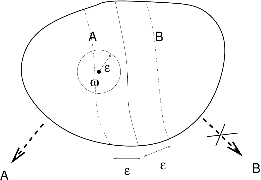
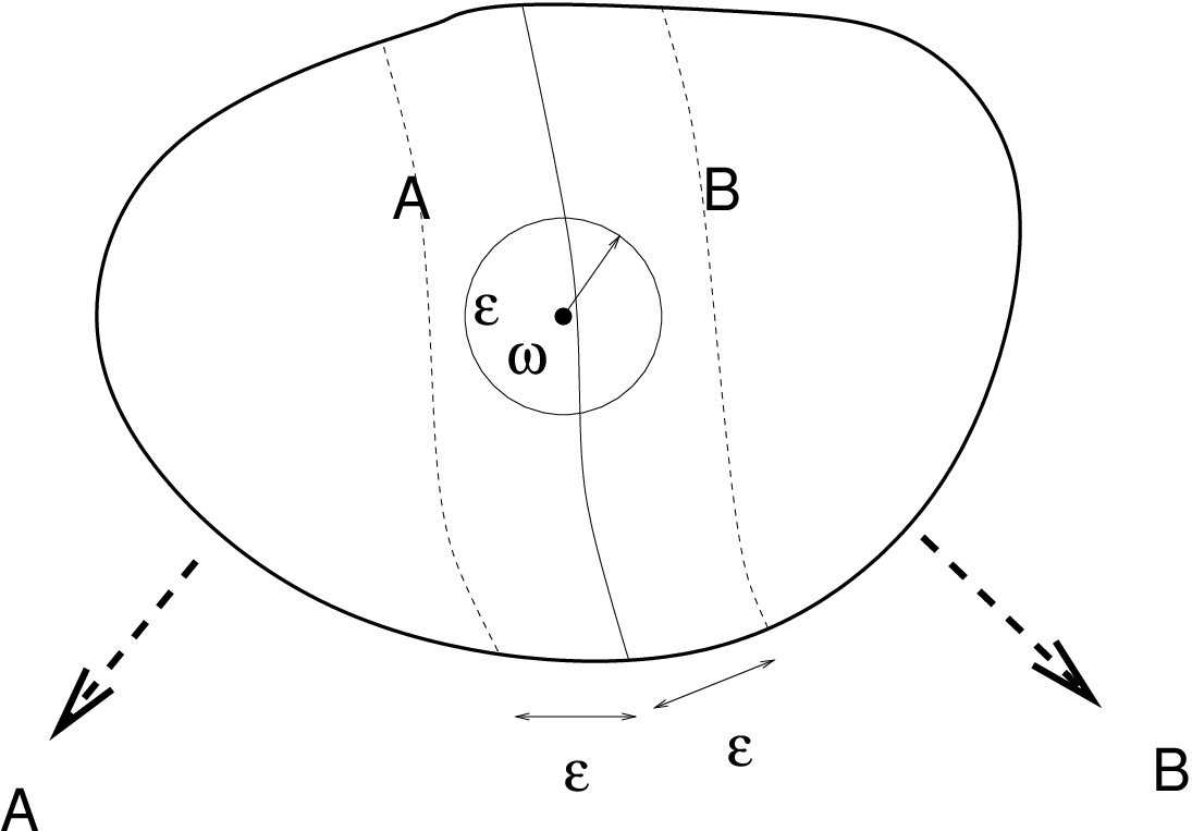
In order to efficiently certify that ${\mathcal{B}}_{\varepsilon}(\omega)\cap B=\emptyset$, one employs the technique of decision functions. A function $f\colon\Omega\to{\mathbb{R}}$ is called 1-Lipschitz if

Assign to every internal mode $C$ a 1-Lipschitz function $f=f_{C}$ so that $f_{C}\upharpoonright B\leq 0$ and $f_{C}\upharpoonright A\geq 0$. It is easily seen that $f_{C}\upharpoonright B_{\varepsilon}<\varepsilon$, and so the fact that $f_{C}(\omega)\geq\varepsilon$ serves as a certificate for ${\mathcal{B}}_{\varepsilon}(\omega)\cap B=\emptyset$, assuring that a sub-tree descending from $B$ can be pruned. Similarly, if $f_{C}(\omega)\leq-\varepsilon$, the sub-tree descending from $A$ can be pruned.

Of course, decision functions should have sufficiently low computational complexity in order for the indexing scheme to be efficient.

A hierarchical indexing structure employing 1-Lipschitz decision functions at every node is known as a metric tree.

Here is a formal definition. A metric tree for a metric similarity workload $(\Omega,\rho,X)$ consists of

• •

  a finite binary rooted tree $\mathcal{T}$,

• •

  a collection of (possibly partially defined) real-valued $1$-Lipschitz functions $f_{t}\colon B_{t}\to{\mathbb{R}}$ for every inner node $t$ (decision functions), where $B_{t}\subseteq\Omega$,

• •

  a collection of bins $B_{t}\subseteq\Omega$ for every leaf node $t$, containing pointers to elements $X\cap B_{t}$,

so that

• •

  $B_{{\mathrm{root}}({\mathcal{T}})}=\Omega$,

• •

  for every internal node $t$ and child nodes $t_{-},t_{+}$, one has $B_{t}\subseteq B_{t_{-}}\cup B_{t_{+}}$,

• •

  $f_{t}\upharpoonright B_{t_{-}}\leq 0$, $f_{t}\upharpoonright B_{t_{+}}\geq 0$.

When processing a range query ${\mathcal{B}}_{\varepsilon}(\omega)$,

• •

  $t_{-}$ is accessed $\iff$ $f_{t}(\omega)<\varepsilon$, and

• •

  $t_{+}$ is accessed $\iff$ $f_{t}(\omega)>-\varepsilon$.

Here is the search algorithm in pseudocode.

Under our assumptions on the metric tree, it can be proved (cf. [34], Theorem 3.3) that Algorithm 3.1 correctly answers every range similarity query for the workload $(\Omega,\rho,X)$, and so together with an indexing scheme forms an access method.

For differing perspectives on metric trees, see [34, 8]. Each of the books [35, 36, 47] is an excellent reference to indexing structures in metric spaces.

In recent years the research emphasis has shifted away from exact towards approximate similarity search:

• •

  given $\varepsilon>0$ and $\omega\in\Omega$, return a point $x\in X$ that is [with confidence $>1-\delta$] at a distance $<(1+\varepsilon)d_{NN}(\omega)$ from $\omega$.

This has led to many impressive achievements, particularly [20, 18], see also the survey [17] and Chapter 7 in [41]. At the same time, research in exact similarity search, especially concerning deterministic algorithms, has slowed down. At a theoretical level, the following unproved conjecture helps to keep research efforts in focus.

The best lower bound currently known is $O(d/\log\frac{sd}{n})$, where $s$ is the number of cells used by the data structure [30]. In particular, this implies the earlier bound $\Omega(d/\log n)$ for polynomial space data structures [3], as well as the bound $\Omega(d/\log d)$ for near linear space (namely $n\log^{O(1)}n$). See also [1, 28, 29]. A general reference for the cell probe model of computation is [24], while in the context of similarity search the model is discussed in [33].

As in [10], we assume the existence of an unknown probability measure $\mu$ on $\Omega$, such that both datapoints $X$ and query points $\omega$ are being sampled with regard to $\mu$.

On the one hand, this assumption is open to debate: for instance, it is said that in a typical university library most books (75 % or more) are never borrowed a single time, so it is reasonable to assume that the distribution of queries in a large dataset will be skewed equally heavily away from data distribution. On the other hand, there is no obvious alternative way of making an apriori assumption about the query distribution, and in some situations the assumption makes sense indeed, e.g. in the context of a large biological database where a newly-discovered protein fragment has to be matched against every previously known sequence.

The triple $(\Omega,\rho,\mu)$ is known as a metric space with measure. This concept opens the way to systematically using the phenomenon of concentration of measure on high-dimensional structures, also known as the “Geometric Law of Large Numbers” [23, 21]. This phenomenon can be informally summarized as follows:

for a typical “high-dimensional” structure $\Omega$, if $A$ is a subset containing at least half of all points, then the measure of the $\varepsilon$-neighbourhood $A_{\varepsilon}$ of $A$ is overwhelmingly close to $1$ already for small $\varepsilon>0$.

Here is a rigorous way for dealing with the phenomenon. Define the concentration function $\alpha_{\Omega}$ of a metric space with measure $\Omega$ by

The value of $\alpha_{\Omega}(\varepsilon)$ gives un upper bound on the measure of the complement to the $\varepsilon$-neighbourhood $A_{\varepsilon}$ of every subset $A$ of measure $\geq 1/2$.

For high-dimensional spaces the values of the concentrataion function often admit gaussian upper bounds of the form

where $d$ is a dimension parameter. For instance, the concentration function of the $d$-dimensional Hamming cube $\{0,1\}^{d}$ with the normalized Hamming metric and uniform measure satisfies a Chernoff bound $\alpha(\varepsilon)\leq\exp(-2\varepsilon^{2}d)$, cf Fig. 5.

Similar bounds hold for Euclidean spheres ${\mathbb{S}}^{n}$, cubes ${\mathbb{I}}^{n}$, and many other structures of both continuous and discrete mathematics, equipped with suitably normalized distances and canonical probability measures. The concentration phenomenon can be now expressed by saying that for “typical” high-dimensional metric spaces with measure, $\Omega$, the concentration function $\alpha_{\Omega}(\varepsilon)$ drops off sharply as $d\to\infty$ [23, 21].

If now $f\colon\Omega\to{\mathbb{R}}$ is a $1$-Lipschitz function, denote $M=M_{f}$ the median value of $f$, that is, a (non-uniquely defined) real number with the property that each of the events $[f\geq M]$ and $[f\leq M]$ occurs with probabiity at least half. One can prove without much difficulty:

Thus, every one-Lipschitz function on a high-dimensional metric space with measure concentrates near one value.

Here are our standing assumptions for the rest of the article. Let $(\Omega,\rho,\mu)$ be a domain equipped with a metric $\rho$ and a probability measure $\mu$. We assume that the expected distance between two points of $\Omega$ is normalized so as to become asymptotically constant:

We further assume that $\Omega$ has “concentration dimension $d$” in the sense that the concentration function $\alpha_{\Omega}$ is gaussian with exponent $\Theta(d)$;

(This approach to intrinsic dimension is developed in [32].)

A dataset $X\subseteq\Omega$ contains $n$ points, where $n$ and $d$ are related as follows:

In other words, asymptotically $n$ grows faster than any polynomial function $Cd^{k}$, $C>0$, $k\in{\mathbb{N}}$, but slower than any exponential function $e^{cd}$, $c>0$. (An example of such rate of growth is $n=2^{\sqrt{d}}$.) For the purposes of asymptotic analysis of search algorithms such assumptions are natural [17].

Datapoints are modelled by a sequence of i.i.d. random variables distributed according to the measure $\mu$:

The instances of datapoints will be denoted with corresponding lower case letters $x_{1},x_{2},\ldots,x_{n}$.

Finally, the query centres $\omega\in\Omega$ follow the same distribution $\mu$:

It is known that in high-dimensional domains the distance to the nearest neighbour is approaching the average distance between two points (cf. e.g. [4] for a particular case). This is a consequence of concentration of measure, and the result can be stated and proved in a rather general situation. Denote $\varepsilon_{NN}(\omega)$ the distance from $\omega\in\Omega$ to the nearest point in $X$. The function $\varepsilon_{NN}$ is easily verified to be $1$-Lipschitz, and so concentrates near its median value. From here, one deduces:

For a proof of Lemma 1, see Appendix A in [33].

This effect is already noticeable in medium dimensions. Let us draw a dataset $X$ with $10,000$ points randomly from the Euclidean cube $[0,1]^{50}$ with regard to the uniform measure. Then, with respect to the usual Euclidean distance, the median value of the distance to the nearest neighbour is $\varepsilon_{M}=1.9701$, while the expected value of a distance between two points of $X$, ${\mathbb{E}}d(x,y)=2.872$. Cf. Fig. 6 for the distribution of values of $\varepsilon_{NN}$.

As a first approximation to our analysis, we present a heuristic argument, allowing linear in $n$ asymptotic lower bounds on the search performance of a metric tree.

What happens at an internal node $C$ when a metric tree is being traversed? Note that $C$ itself becomes a metric space with measure if equipped with the metric induced from $\Omega$ and a probability measure $\mu_{C}$ which is the normalized restriction of the measure $\mu$ from $\Omega$:

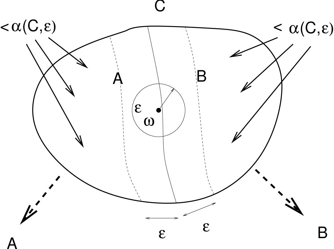
Let $\alpha_{C}$ denote the concentration function of $C$. Suppose for the moment that our tree is perfectly balanced: $\mu_{C}(A)=\mu_{C}(B)=\frac{1}{2}$. Then the size of the $\varepsilon$-neighbourhood of $A$ is at least $1-\alpha_{C}(\varepsilon)$, and the same is true of $B_{\varepsilon}$. For all query points $\omega\in C$ except a set of measure $\leq 2\alpha_{C}(\varepsilon)$, the search algorithm 3.1 branches out at the node $C$. (Cf. Fig. 7.)

Let $\mathscr{C}$ be a family of subsets of a set $\Omega$ (a concept class). One says that a subset $A\subseteq\Omega$ is shattered by $\mathscr{C}$ if for each $B\subseteq A$ there is $C\in{\mathscr{C}}$ such that

The Vapnik–Chervonenkis dimension ${\mathrm{VC}}({\mathscr{C}})$ of a class $\mathscr{C}$ is the supremum of sizes of finite subsets $A\subseteq\Omega$ shattered by $\mathscr{C}$.

Here are some examples.

1. 1.

   The VC dimension of the class of all Euclidean balls in ${\mathbb{R}}^{d}$ is $d+1$.

2. 2.

   The class of all parallelepipeds in ${\mathbb{R}}^{d}$ has VC dimension $2d+2$.

3. 3.

   The VC dimension of the class of all balls in the Hamming cube $\{0,1\}^{d}$ is bounded from above by $d+\lfloor\log_{2}d\rfloor$.

   (As every ball is determined by its centre and radius, the total number of pairwise different balls in $\{0,1\}^{d}$ is $d2^{d}$. Now one uses an obvious observation: the VC dimension of a finite concept class $\mathscr{A}$ is bounded above by $\log_{2}\left|\mathscr{A}\right|$.)

Here is a deeper result.

Here is a typical result of statistical learning theory, which we quote from [42], Theorem 7.8.

Let $\mathscr{F}$ be a class of (possibly partially defined) real-valued functions on $\Omega$. Define ${\mathscr{F}}_{\geq}$ as the family of all sets of the form

The value of ${\mathrm{VC}}({\mathscr{F}}_{\geq})$ is bounded above by the Pollard dimension (pseudodimension) of $\mathscr{F}$ (cf. [42], 4.1.2), but is in general smaller.

For both schemes, if $\Omega={\mathbb{R}}^{d}$ or $\{0,1\}^{n}$, then ${\mathrm{VC}}(({\mathscr{F}})_{\geq})$ equals $d+1$. A similar conclusion holds for the Hamming cube.

In this Section we prove the following theorem under general assumptions of Section 7.

The following is a direct application of Lemma 4.2 in [31].

Here is the next step in the proof.

In this Section, written in response to referee’s comments, the author will try to outline his understanding of applicability of the method of proof to other indexing paradigms.

The approach to obtaining lower bounds on performance of indexing schemes adopted in this paper consists in combining simple concentration of measure considerations with the basic techniques of statistical learning (VC theory). The argument is applicable to the situation of the following kind. Let $W=(\Omega,\rho,X)$ denote a similarity workload. An indexing scheme for $W$ consists of a family of real-valued $1$-Lipschitz functions $f_{i}$, $i\in I$ on $\Omega$, which are in general partially defined: ${\mathrm{dom}}\,(f_{i})\subseteq\Omega$. Given a query $(\omega,\varepsilon)$, where $\omega\in\Omega$ and $\varepsilon>0$, the algorithm chooses recursively a sequence of indices $i_{n}$, based on the previous values $f_{i_{k}}(\omega)$, $k<n$. At some point, the computation is terminated, and the values $f_{i_{k}}(\omega)$ point at a collection of bins, whose contents are read off. The role of the functions $f_{i}$ is to discard those datapoints (or the entire bins) which cannot possibly answer the query. Namely, if $\left|f_{i}(\omega)-f_{i}(x)\right|\geq\varepsilon$, then, since $f_{i}$ is a $1$-Lipschitz function, one has $d(\omega,x)\geq\varepsilon$, and so the point $x$ is irrelevant. All the points (or entire bins) which cannot be discarded are returned and their contents checked against the condition $d(x,\omega)<\varepsilon$.

On the spaces of high dimension, every $1$-Lipschitz function concentrates sharply near its mean (or median) value. If in addition we assume that the class $\mathscr{F}$ of all functions used for a particular indexing scheme has a low complexity in the sense of VC dimension, we can conclude that the number of points discarded by every function $f_{i}$ drops off fast as dimension $d$ of the domain grows, resulting in degrading performance.

So far, we are aware of essentially two different types of such indexing schemes: metric trees (treated in the present paper) and pivot tables [6]. For pivots, the methods of the present paper have been subsequently used to derive an expected average performance lower bound $\Omega\left({n}/{d\log n}\right)$ [43]. It is not clear to the author how to state a more general result from which both estimates would follow, nor whether such a result would be useful in view of lack of other examples.

Even if the cell-probe model has some formal similarities with the metric tree scheme (a hierarchical tree structure, a collection of cells as an indexing scheme, computations performed at each node with a limited number of cells accessed, etc.), it is not clear whether the partially defined functions determined by the algorithm at each node will be $1$-Lipschitz (they are taking values in the Hamming cube). The examples of implemented indexing schemes for exact nearest neighbour search known to this author seem to be using $1$-Lipschitz functions, but of course this does not preclude the existence of schemes based on other ideas.

Furthermore, assuming that an indexing scheme consists of a family of $1$-Lipschitz functions whose values are recursively computed by the algorithm does not necessarily imply that the role of the functions is reduced to certifying that a certain point is not in the $\varepsilon$-ball around the query point. As an example, consider the indexing scheme [11] based on a walk on the Delaunay graph of $X$ in $\Omega$ and called spatial approximation in [25]. For every datapoint $x\in X$, the scheme stores a list of datapoints whose Voronoi cells are adjacent to the cell containing $x$. At the search phase, a sequence of datapoints $x_{1},x_{2},\ldots,x_{n}$ is chosen, where each $x_{i+1}$ is the closest point to $\omega$ on the list of points Delaunay-adjacent to $x_{i}$. If choosing $x_{i+1}$ so as to get closer to $\omega$ is impossible, one backtracks. In practice, the scheme performs on par with the state of the art pivot or metric tree based schemes [27]. We do not know whether our methods can be employed to prove the curse of dimensionality for this particular scheme in the same general setting.

It appears that attempting to extend the method to randomized, approximated NN search stands no chance either. Firstly, the dimensionality reduction-type methods often present in randomized algorithms for approximate search [20, 18, 1] mean that instead of $1$-Lipschitz functions, one is using what may be called “probably approximately $1$-Lipschitz” ones. For instance, a random projection from a high-dimensional Euclidean space to a subspace of smaller dimension, appropriately rescaled, will have the property that for most pairs of points $x,y$ the distance between them is approximately preserved, to within a factor of $1\pm\varepsilon$. This property in itself is a consequence of concentration of measure, but such maps do not exhibit a strong concentration property, rendering our methods inapplicable.

Chapter 4 in [47] discusses algorithms for approximate similarity search based on a traditional metric tree, equipped with $1$-Lipschitz decision functions, but employing agressive pruning, either randomized or deterministic. Even here, our proof does not seem to be readily transferable. Indeed, it is based on the basic premise that every bin meeting the $\varepsilon$-neighbourhood of the query point needs to be examined in a deterministic fashion. A randomized algorithm, on the contrary, avoids opening bins which are deemed unlikely to contain relevant datapoints. Experiments confirm that some of the algorithms in question perform up to 300 times faster than the corresponding algorithms for exact search using the same indexing structure (loc.cit.), and provide a circumstantial evidence that the situation here is indeed fundamentally different and possibly not amenable to the same methods of analysis.

While the setting of artificially high-dimensional synthetic i.i.d. data fed to a scheme is not realistic, our results provide a theoretical validation to the known simulation results on the poor performance in medium to high dimensions of metric-tree type indexing schemes, such as SS tree [45] and SR tree [19], on such data inputs.

Some data practitioners believe that the intrinsic dimension of real-life datasets does not exceed as few as perhaps seven or ten dimensions. A deeper understanding of underlying geometry of workloads and its interplay with compleixty is called for in order to learn to detect and use this low dimensionality efficiently, and asymptotic analysis of algorithm performance in an artificial setting of very high dimensions is contributing towards this goal.

References

- (1) A. Andoni, P. Indyk, M. Pǎtrascu, On the optimality of the dimensionality reduction method, in: Proc. 47th IEEE Symp. on Foundations of Computer Science, pp. 449–458, 2006.
- (2) M. Anthony and P. Bartlett. Neural Network Learning: Theoretical Foundations. Cambridge University Press, Cambridge, 1999.
- (3) O. Barkol and Y. Rabani. Tighter lower bounds for nearest neighbor search and related problems in the cell probe model. In: Proc. 32nd ACM Symp. on the Theory of Computing, 2000, pp. 388–396.
- (4) K. Beyer, J. Goldstein, R. Ramakrishnan, and U. Shaft. When is “nearest neighbor” meaningful?, in: Proc. 7-th Intern. Conf. on Database Theory (ICDT-99), Jerusalem, pp. 217–235, 1999.
- (5) A. Borodin, R. Ostrovsky, and Y. Rabani. Lower bounds for high-dimensional nearest neighbor search and related problems, in: Proc. 31st Annual ACS Sympos. Theory Comput., 312–321, 1999.
- (6) Bustos, B., Navarro, G., Chávez, E. (2003) Pivot selection techniques for proximity searching in metric spaces. Pattern Recognition Lett., vol. 24, pp. 2357–2366.
- (7) E. Chávez, G. Navarro. A compact space decomposition for effective metric indexing. Pattern Recognition Letters 26:1363–1376, 2005.
- (8) E. Chávez, G. Navarro, R. Baeza-Yates and J. L. Marroquín. Searching in metric spaces. ACM Computing Surveys 33:273–321, 2001.
- (9) P. Ciaccia, M. Patella and P. Zezula. M-tree: An efficient access method for similarity search in metric spaces. In Proc. 23rd Int. Conf. on Very Large Data Bases (VLDB’97), (Athens, Greece), 426–435, 1997.
- (10) P. Ciaccia, M. Patella and P. Zezula. A cost model for similarity queries in metric spaces, in: Proc. 17-th ACM Symposium on Principles of Database Systems (PODS’98), Seattle, WA, 59–68, 1998.
- (11) K.L. Clarkson. An algorithm for approximate closest-point queries. In: Proc. 10th symp. Comp. Geom. Stony Brook, NY, 160–164, 1994.
- (12) K.L. Clarkson. Nearest-neighbor searching and metric space dimensions. In: Nearest-Neighbor Methods for Learning and Vision: Theory and Practice, MIT Press, 2006, pp. 15–59.
- (13) A. Faragó, T. Linder, and G. Lugosi, Fast nearest neighbor search in dissimilarity spaces, IEEE Transactions on Pattern Analysis and Machine Intelligence, vol. 18, pp. 957–962, 1993.
- (14) P.W. Goldberg and M.R. Jerrum, Bounding the Vapnik–Chervonenkis dimension of concept classes parametrized by real numbers, Machine Learning 18:131-148, 1995.
- (15) M. Gromov and V.D. Milman, A topological application of the isoperimetric inequality. Amer. J. Math. 105, 843–854, 1983.
- (16) J. M. Hellerstein, E. Koutsoupias, D. P. Miranker, C. Papadimitriou, and V. Samoladas. On a model of indexability and its bounds for range queries. Journal of the ACM (JACM), 49(1):35–55, 2002.
- (17) P. Indyk. Nearest neighbours in high-dimensional spaces. In: J.E. Goodman, J. O’Rourke, Eds., Handbook of Discrete and Computational Geometry, Chapman and Hall/CRC, Boca Raton–London–New York–Washington, D.C. 877–892, 2004.
- (18) Piotr Indyk, Rajeev Motwani, Approximate nearest neighbors: towards removing the curse of dimensionality, Proceedings of the thirtieth annual ACM symposium on Theory of computing, pp. 604–613, 1998, Dallas, Texas.
- (19) N. Katayama and S. Satoh, The -tree: An index structure for high-dimensional nearest neighbour queries, in: Prof. 16-th Symposium on PODS, pp. 369–380, Tuscon, AZ, 1997.
- (20) E. Kushilevitz, R. Ostrovsky, Y. Rabani, Efficient Search for Approximate Nearest Neighbor in High Dimensional Spaces. SIAM Journal on Computing 30:457–474, 2000.
- (21) M. Ledoux. The Concentration of Measure Phenomenon, volume 89 of Mathematical Surveys and Monographs. American Mathematical Society, Providence, RI, 2001.
- (22) S. Mendelson, A few notes on statistical learning theory. In: S. Mendelson, A.J. Smola, Eds., Advanced Lectures in Machine Learning, LNCS 2600, pp. 1–40, Springer, 2003.
- (23) V.D. Milman and G. Schechtman, Asymptotic Theory of Finite Dimensional Normed Spaces, volume 1200 of Lecture Notes in Mathematics. Springer, 1986.
- (24) P.B. Miltersen, Cell probe complexity - a survey. In: 19th Conference on the Foundations of Software Technology and Theoretical Computer Science (FSTTCS), 1999. Advances in Data Structures Workshop.
- (25) Gonzalo Navarro, Searching in metric spaces by spatial approximation, The VLDB Journal 11:28–46, August 2002.
- (26) Gonzalo Navarro, Analysing metric space indexes: what for? Invited paper, in: Proc. 2nd Int. Workshop on Similarity Search and Applications (SISAP 2009), Prague, Czech Republic, 2009, 3–10.
- (27) Gonzalo Navarro, Nora Reyes, Dynamic spatial approximation trees for massive data, in: Proc. 2nd Int. Workshop on Similarity Search and Applications (SISAP 2009), Prague, Czech Republic, 2009, pp. 81–88.
- (28) R. Panigrahy, K. Talwar, U. Wieder, A geometric approach to lower bounds for approximate near-neighbor search and partial match, in: Proc. 49th IEEE Symp. on Foundations of Computer Science, pp. 414–423, 2008.
- (29) R. Panigrahy, K. Talwar, U. Wieder, Lower bounds on near neighbor search via metric expansion, in: Foundations of Computer Science (FOCS 2010), pp. 805–814.
- (30) M. Pǎtrascu, M. Thorup, Higher lower bounds for near-neighbor and further rich problems, in Proc. 47th IEEE Symp. on Foundations of Computer Science, pp. 646–654, 2006.
- (31) V. Pestov. On the geometry of similarity search: dimensionality curse and concentration of measure. Inform. Process. Lett., 73:47–51, 2000.
- (32) V. Pestov. An axiomatic approach to intrinsic dimension of a dataset. Neural Networks, 21:204–213, 2008.
- (33) V. Pestov. Indexability, concentration, and VC theory. Journal of Discrete Algorithms, doi:10.1016/j.jda.2011.10.002.
- (34) V. Pestov and A. Stojmirović. Indexing schemes for similarity search: an illustrated paradigm. Fund. Inform., 70:367–385, 2006.
- (35) H. Samet. Foundations of Multidimensional and Metric Data Structures. Morgan Kaufmann Publishers Inc., San Francisco, CA, 2005.
- (36) S. Santini, Exploratory Image Databases: Content-Based Retrieval, Academic Press, Inc. Duluth, MN, USA, 2001.
- (37) U. Shaft and R. Ramakrishnan. Theory of nearest neighbors indexability. ACM Transactions on Database Systems (TODS), 31:814–838, 2006.
- (38) A. Stojmirović and V. Pestov. Indexing schemes for similarity search in datasets of short protein fragments. Information Systems, 32:1145–1165, 2007.
- (39) J.K. Uhlmann. Satisfying general proximity/similarity queries with metric trees, Information Processing Letters 40:175–179, 1991.
- (40) V.N. Vapnik. Statistical Learning Theory. John Wiley & Sons, Inc., New York, 1998.
- (41) S.S. Vempala. The Random Projection Method. DIMACS Series in Discrete Mathematics and Theoretical Computer Science, 65, Amer. Math. Soc., Providence, R.I., 2004.
- (42) M. Vidyasagar. Learning and Generalization, With Applications to Neural Networks. Second Ed. Springer-Verlag, London, 2003.
- (43) I. Volnyansky and V. Pestov, Curse of dimensionality in pivot-based indexes. - Proc. 2nd Int. Workshop on Similarity Search and Applications (SISAP 2009), Prague, Czech Republic, 2009, pp. 39-46.
- (44) R. Weber, H.-J. Schek, and S. Blott, A quantatitive analysis and performance study for similarity-search methods in high-dimensional spaces. in: Proceedings of the 24-th VLDB Conference, New York, pp. 194–205, 1998.
- (45) D.A. White and R. Jain, Similarity indexing with the -tree, in: Proc. 12th Conf. on Data Engineering (ICDE’96), La Jolla, CA, pp. 516–523, 1996.
- (46) P. Yianilos. Data structures and algorithms for nearest neighbor search in general metric spaces, in: Proc. 3rd Annual ACM-SIAM Symposium on Discrete Algorithms, pp. 311–321, 1993.
- (47) P. Zezula, G. Amato, Y. Dohnal, and M. Batko. Similarity Search. The Metric Space Approach. Springer Science Business Media, New York, 2006.