Quantum transfer matrix method for one-dimensional disordered electronic systems
Abstract
We develop a novel quantum transfer matrix method to study thermodynamic properties of one-dimensional (1D) disordered electronic systems. It is shown that the partition function can be expressed as a product of local transfer matrices. We demonstrate this method by applying it to the 1D disordered Anderson model. Thermodynamic quantities of this model are calculated and discussed.
pacs
63.50.+x, 02.30.Ik, 71.23.AnI Introduction
For real solids, the perfect periodicity is an idealization, while the imperfections are of great importance for transport properties. The broken translational symmetry makes the system deviate from the extended Bloch waves behavior, and in some cases, to localized states. As pointed out in Ref. [1], we can not adopt the model of ordered systems to understand disordered materials. The concept of Anderson localization [2] and the correlation effect [3] among electrons in a disordered medium are two important ingredients in the understanding of disordered systems.
As a minimal Hamiltonian for independent electrons in a disordered potential, the Anderson disordered model remains difficult to be understood in finite temperature. The disorder itself invalidates conventional analytical methods. No proper perturbation parameter can be chosen to deal with disordered Hamiltonian although perturbation theory was applied to calculate the conductivity in weak disorder limit. Considerable efforts focus on Anderson localization and corresponding metal-insulator transition. In particular, much insight was gained from the scaling analysis[4, 5].
In contrast to higher dimensional cases, 1D models are often accessible to obtain detailed theoretical (analytical and numerical) results. However, in the disordered case, it is intractable to make calculation in the thermodynamic limit by analytical methods even in 1D. The aim of this work is to develop a novel method to resolve this technical problem. Our method avoids direct diagonalization of the Hamiltonian and allows the thermodynamic limit to be explored directly and accurately. The key point lies in the fact that we can exploit the full translational symmetry in the Trotter (imaginary time or inverse temperature) direction after trading the evolution in real space direction with the Trotter one.
It should be noted that the transfer matrix introduced in the present scheme is not the one usually used in the study of disordered systems [6]. Our starting point is to express the partition function of the system analytically in terms of the transfer matrix, rather than to use it to trace the eigenvalues or wave functions.
We will take the disordered Anderson model as an example to demonstrate how the quantum transfer matrix method works. The Hamiltonian is defined by
| (1) |
where is the hopping integral between two adjacent sites, is a fermion annihilation(creation) operator at site , is the diagonal disordered potential, and is the chemical potential. and can take random values satisfying some distributions, respectively.
II Quantum Transfer matrix method
As in the quantum transfer matrix renormalization group(TMRG) [7, 8, 9] method, we first separates into two parts, , with each part a sum of commuting terms:
| (2) |
where
| (3) |
The TMRG uses the second-order approximation of the Trotter-Suzuki formula[10, 11]
| (4) |
where and is the temperature. is then divided into parts uniformly, and is the Trotter number.
| (5) |
where are the local evolution operators defined by . By inserting identities
| (6) |
between the neighboring and operators in (4) and labeling successively the complete bases with (so called imaginary time’s slices), the partition function can then be expressed as
| (7) | |||||
where represents the matrix element of . The subscripts and superscripts for and stand for the coordinates in the real and Trotter directions, respectively. If we collect all with the same , the partition function can be re-expressed as the column quantum transfer operators [11, 12]:
| (8) |
In Eq. (8), there exist site-dependent column transfer operators , which are defined by a product of local transfer operators,
| (9) |
where the matrix element of the local transfer operator is defined by
| (10) |

The evolution of this matrix is illustrated in Fig. (1). The reason for labeling the basis state by is to ensures the conservation of the total occupation number of two adjacent sites in the Trotter direction. Since conserves the total occupation number at sites and , subspaces , and are decoupled. In writing Eq. (7), a periodic boundary condition is imposed in the Trotter direction.
Now let uf introduce the following site-dependent variables:
| (11) |
Only three of which are independent. In terms of these variables, we obtain the following matrix elements for in the state number representation :
| (12) |
According to the procedure mentioned above, the resulting local transfer matrix in the Trotter direction between slices and is also block-diagonal because of the fermion number conservation. Consequently,
| (13) |
It can be shown that this transfer matrix has the following operator form:
| (14) | |||||
where ’s are fermion operators defined in the Trotter space. is a quadratic function of fermion operators. Furthermore, can be exponentiated again to a concise quadratic form due to the fermion exclusion principle. For simplicity, we denote , , and
| (15) |
then,
This exponential quadratic operator form of is valid only when the four coefficients before , , , and satisfy the following four equations:
| (17) |
Now we can cast the column transfer matrix defined by Eq. (9) into the following form:
| (18) | |||||
is translational invariant in the Trotter direction. Therefore, we can introduce a fourier transformation along this direction:
| (19) |
The general column transfer matrix can then be rewritten as
Substituting these transfer matrices into Eq. (8), we obtain the following expression for the partition function:
| (27) |
where
| (28) |
and are matrices defined by
In obtaining these expressions, we have used the fact that is an identity matrix in the subspace , . In Eq. (28), all multiplied matrices are exponential of traceless matrices. Thus the eigenvalue of the final matrix after multiplications will have the form . In the thermodynamic limit, the constant in Eq. (28) can be neglected because the eigenvalue dominates.
It should be noted that is related to the parity of . For odd
| (35) |
and for even
| (36) |
The transfer matrix in Eq. (28) is calculated in the subspace of , so the fermion occupation number is 1 for each two unit cells along the Trotter direction. The state space for one column transfer matrix is
| (37) |
and the total occupation number is . Due to the periodicity in Trotter direction, it is equivalent to calculate in the state space
| (38) |
However, permuting the fermion operator behind will bring factor because of the transposition with occupied fermions. Therefore, there are the relation,
| (39) |
For odd , ; For even , . As a result, takes values according to the formulas (35) and (36) respectively. In the following, we will set to even and use Eq. (36).
As shown in Ref. [13], in Eq. (28) can be formally regarded as the transfer matrix for the following 1D Ising model in a magnetic field:
| (40) |
For the odd sites, the parameters are -independent in the corresponding 1D Ising model with the relations
| (41) | |||||
| (42) | |||||
| (43) |
However, the situation is different for even sites and the parameters , are now -dependent
| (44) | |||||
| (45) | |||||
| (46) |
The correspondence for even sites cannot provide a material mapping to 1D Ising model because of the complex parameters, which arises from the fourier transformation along the Trotter direction. Since there exists a relation due to the factor , we can multiply in pair the transfer matrices with and . In fact, the pairwise multiplication can save us half of the calculation because of the complex conjugate relation. When using Eq. (28) to solve the partition function, what is needed is to calculate the product of matrices of dimension for a given . When is obtained, the calculation of the free energy is direct, (hereafter taking ), with which all other thermodynamic quantities interested such as the specific heat can be obtained.
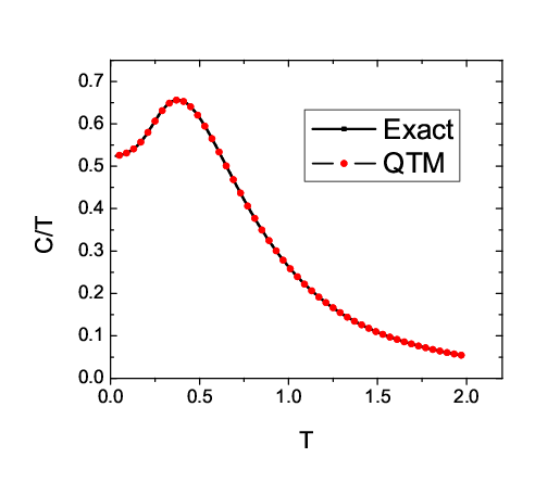
Fig. 2 shows the result of this comparison for the linear coefficient of the specific heat . It is obvious that the two sets of data coincide completely. The chain length here and in the rest of the paper is taken up to .
III Results
III.1 Gaussian diagonal disorder
We first consider a Gaussian-like function
| (47) |
for the disordered distribution of the diagonal potential , where and are the mean value and the standard deviation respectively. In the following discussion, we take , , . The controlling parameter is the standard deviation , which denotes the disorder degree of the distribution of . In these figures, the red solid line means the case without disorder, i.e. (), and the other curves are for and .


As shown in Figs. 3-5, the difference of the physical quantities is slight between the cases of and . However, significant differences appear when increases. With increasing , the peaks of the specific heat move towards higher temperatures. The introduction of disordered diagonal energy widens the energy band. The density of states(DOS) distributes in a broaden energy range. This leads to the shift of the peak position of towards higher temperature with increasing . The disorder assists the thermal fluctuations and shifts the peak of to lower temperatures. The specific heat coefficient at zero temperature is proportional to the density of states around the Fermi energy , i.e.,
| (48) |
Fig. 4 shows that when the disorder increases, the density of state near the fermi surface decreases. The entropy decreases when increases.
Fig. 6 shows how the chemical potential changes with for some given occupation numbers . becomes large with increasing when keeps invariant, while become small with increasing when keeps intact. To keep invariant, is a monotonic increasing function of . The function shows linear shape at high temperature regime.

In Eq. (27), the partition function is expressed as product of different components, consequently, the free energy can be written as a sum of dependent free energy . For a given temperature , decreases with increasing. When the disorder is turned on, changes little except in the vicinity of . This can be seen from Fig. 7, which compares the difference of free energies between the disordered () and ordered cases as a function of . It clearly shows that the difference becomes significant only when approaches . In Ref. [13], the singularity from some special ’s was used to discuss the phase transition.

III.2 Staggered disorder potential
We now consider a special model whose diagonal potential energy is alternating (staggered) with the lattice site, i.e.,
| (49) |
When , the energy spectrum is readily calculated via the Fourier transformation,
| (50) |
The result is two sub-bands dispersion relation,
| (51) |
The band gap is .
Let us choose a uniform rectangular distribution for the increment of the random diagonal energy . Here, is the width of the rectangular distribution satisfying
| (52) |
In the presence of disorder, the band gap is expected to decrease with the increase of the disorder degree . For small , there is a finite excitation gap and the specific heat drops exponentially in low temperature, as shown in Fig. 8 .

We also consider the case when the random potential take only two discrete values: with equal probability. We call it discrete distribution of the increment, and the above rectangular distribution is denoted by continuous one.
Fig. 9 compares the specific heat coefficient at for the above two kinds of distribution of random potentials. In the case of discrete distribution, exhibits a sharper peak. When the disordered level increases to approximately , the band gap disappears. With further increasing , drops to zero because the band gap open again for the discrete random potential. This can be understood as follows. The two sub-bands close to each other when disorder is introduced. The upper sub-band shifts downwards by and the lower sub-band shifts upwards by . When the top of the original upper sub-band touches the zero energy, i.e., , the two sub-bands begin to separate again. Therefore, decreases to zero at in Fig. 9. On the contrary, for the continuous random increment case, remains a finite value even for large . This is because the splitting of the upper and lower bands only blurringly expands the width of these two bands, and once they touch each other, they never separate again.

As a further investigation for in discrete distribution, we choose three typical disordered degrees , corresponding to three regions in Fig. 9, to show how varies with the temperature at low .
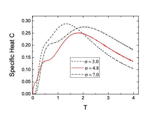
As shown in Fig. 10, when and 7.0, drops exponentially with temperature in low temperatures. The double-peak structure of can be understood from the overlaps of energy bands. The discrete increments split the original single energy band into the two bands which shift upwards and downwards by . The resulting four bands from upper and lower sub-bands meet pairwise. The thermal fluctuations bring double peaks shown in curves.
IV conclusion
For the 1D disordered system, the quantum transfer matrix method we have developed is applicable to all kinds of disorder distribution types and strengths. The non-diagonal disordered problem can be handled since the partition function can be expressed as the product of site-dependent local transfer matrices. Compared to the diagonal disordered cases, we only need to modify the local transfer matrix elements correspondingly.
We have studied the thermodynamic properties of the 1D disordered Anderson model. We discussed two kinds of diagonal (potential) disordered models with or without staggered potentials. The free energy can be written as a sum of different components from the Fourier transformation in Trotter space. Comparing with the system without disorder, the most significant difference in shows only in the region very close to . The disorder change the distribution of DOS, leading to the difference in the thermodynamic quantities in comparison with the disorder-free system. All the results shown in the figures are for systems with the number of sites greater than . This kind of calculation is far beyond the capacity of exact diagonalization.
The transfer matrix method has a broad range of applicability and can be used to discuss any non-interacting fermion models. Recently this method has been used to calculate the thermodynamic quantities of the Hofstadter model which describes the behavior of tightly-bound Bloch electrons in the magnetic field [14, 15]. In Landau gauge, the Hofstadter Hamiltonian can be decoupled into a sum of one dimensional Hamiltonian, which lies in the application range of the quantum transfer matrix method.
Acknowledgements.
This work was supported by the National Natural Science Foundation of China and the National Program for Basic Research of MOST, China.References
- [1] P. A. Lee and T. V. Ramakrishnan, Rev. Mod. Phys. 57, 287 (1985).
- [2] P. W. Anderson, Phys. Rev. 109, 1492 (1958).
- [3] B. L. Altshuler and A. G. Aronov, Solid State Commun. 39, 115 (1979).
- [4] F. Wegner, Z. Phys. B 25, 327 (1976).
- [5] E. Abrahams, P. W. Anderson, D. C. Licciardello, and T. V. Ramakrishnan, Phys. Rev. Lett. 42, 673 (1979).
- [6] T. Brandes and S. Kettemann, Anderson Localization and Its Ramifications, (Springer, Berlin, 2003).
- [7] R. J. Bursill, T. Xiang, and G. A. Gehring, J.Phys.: Condens. Matter 8, L583 (1996).
- [8] X. Q. Wang and T. Xiang, Phys. Rev. B 56, 5061 (1997).
- [9] T. Xiang and X. Wang, in Density-Matrix Renormalization: A New Numerical Method in Physics, edited by I. Peschel, X. Wang, M. Kaulke, and K. Hallberg (Springer, New York, 1999), pp. 149-172.
- [10] H. F. Trotter, Proc. Am. Math. Soc. 10, 545 (1959).
- [11] M. Suzuki, Prog. Theor. Phys. 56, 1454 (1976).
- [12] H. Betsuyaku, Prog. Theor. Phys. 73, 320 (1985).
- [13] R. Shankar and G. Murthy, Phys. Rev. B 36, 536 (1987).
- [14] W. H. Xu, L. P. Yang, M. P. Qin and T. Xiang, arXiv: 0808.0099 (2008).
- [15] L. P. Yang and T. Xiang, unpublished.