Global Phase Diagram for Magnetism and Lattice Distortion of
Fe-pnictide Materials
Abstract
We study the global phase diagram of magnetic orders and lattice structure in the Fe-pnictide materials at zero temperature within one unified theory, tuned by both doping and pressure. On the low doping and high pressure side of the phase diagram, there is one single transition, which is described by a mean field theory with very weak run-away flows; on the high doping and low pressure side the transition is expected to split to two transitions, with one O(3) spin density wave transition followed by a quantum Ising transition at larger doping. The fluctuation of the strain field fluctuation of the lattice will not affect the spin density wave transition, but will likely drive the Ising nematic order transition more mean field like through a linear coupling, as observed experimentally in .
I I, Introduction
The Iron-superconductor, for its potential to shed new light on the non-BCS type of superconductors, has attracted enormous interests since early this year. Despite the complexities and controversies on the superconducting mechanism, the minimal tight-binding model, or even the exact pairing symmetry of the cooper pair, these samples do share two common facts: the tetragonal-orthorhombic lattice distortion and the spin density wave (SDW) [2]. Both effects are suppressed under doping and pressure, and they seem always to track each other in the phase diagram. In Ref. [16, 17], the lattice distortion is attributed to preformed spatially anisotropic spin correlation between electrons, without developing long range SDW the lattice distortion and SDW both stem from magnetic interactions. More specifically, the Ising order parameter is represented as , and are two Neel orders on the two different sublattices of the square lattice.
Since this order deforms the electron Fermi surface, equivalently, it can also be interpreted as electronic nematic order. The intimate relation between the structure distortion and SDW phase has gained many supports from recent experiments. It is suggested by detailed X-ray, neutron and Mössbauer spectroscopy studies that both the lattice distortion transition and the SDW transition of are second order [18], where the two transitions occur separately. However, in undoped with , the structure distortion and SDW occur at the same temperature, and the transition becomes a strong first order transition [4, 5, 6, 7, 8]. Also, recent neutron scattering measurements on indicate that in this material the SDW wave vector is for both sublattices [25] instead of as in 1111 and 122 materials, and the low temperature lattice structure is monoclinic instead of orthorhombic (choosing one-Fe unit cell). These results suggest that the SDW and structure distortion are indeed strongly interacting with each other, and probably have the same origin. The sensitivity of the location of the lattice distortion transition close to the quantum critical point against the external magnetic field (magnetoelastic effect) can further confirm this unified picture.
The clear difference between the phase diagrams of 1111 and 122 materials can be naturally understood in the unified theory proposed in Ref. [16, 17]. We can write down a general Ginzburg-Landau mean field theory for , and :
| (1) | |||||
| (3) |
and are tuned by the temperature. For a purely two dimensional system, the Ising order which induces the lattice distortion occurs at a temperaure controlled by the inplane spin coupling , while there is no SDW transition at finite temperature; for weakly coupled two dimensional layers, the Ising transition temperature is still of the order of the inplane coupling, while the SDW transition temperature is , with representing the interlayer coupling. This implies that on quasi two dimensional lattices, , or is large in the Ginzburg-Landau mean field free energy in Eq. 3. In real systems, The 1111 materials are much more anisotropic compared with the 122 materials, since the electron band structure calculated from LDA shows a much weaker direction dispersion compared with the 122 samples [27]; also the upper critical field of 122 samples is much more isotropic [26]. This justifies treating the 1111 materials as a quasi two dimensional system, while treating the 122 materials as a three dimensional one. When and are close enough, is small, and the interaction between the Ising order parameter and the SDW will drive the transition first order by minimizing the free energy Eq. 3. The phase diagram of free energy Eq. 3 is shown in Fig. 1.

Motivated by more and more evidences of quantum critical points in the Fe-pnictides superconductors [9, 10, 3, 11, 12, 13], in this work, we will explore the global phase diagram of magnetic and nematic orders at zero temperature, tuned by two parameters, pressure and doping. In section II we will study the phase diagram for quasi two dimensional lattices, with applications for 1111 materials, and in section III the gear will be switched to the more isotropic 3d lattices of 122 materials. Section IV will briefly discuss the effect of the coupling between the Ising transition and the strain tensor of the lattice, which will drive the finite temperature Ising nematic transition a mean field transition, while the SDW transition remains unaffected, as observed in [11]. The analysis in our current work are all only based on the symmetry of the system, and hence independent of the details of the microscopic model.
II II, quasi two dimensional lattice
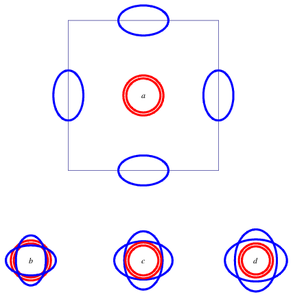
In Ref. [16], the zero temperature quantum phase transition was studied for weakly coupled 2d layers with finite doping. Since the hole pockets and the electron pockets have small and almost equal size, the slight electron doping would change the relative size of the electron and hole pockets substantially. Also, the neutron scattering measurement suggests that the SDW order wave vector is independent of doping in 1111 materials [3]. Therefore under doping the low energy particle-hole pair excitations at wave vector are lost very rapidly, and the spin density wave order parameter at low frequency and long wavelength limit can no longer decay with particle-hole pairs (the fermi pockets are schematically showed in Fig. 2). After integrating out electrons we would obtain the following Lagrangian [16]:
| (4) | |||||
| (6) |
which contains no damping term. The first three terms of the Lagrangian describe the two copies of 3D O(3) Neel orders on the two sublattices. The term is the only relevant term at the 3D O(3) transition, since it has positive scaling dimension [33]. We expect this term to split the two coinciding O(3) transitions into two transitions, an O(3) transition and an Ising transition for Ising variable , as observed experimentally in 1111 materials [3].
The two transitions after splitting are an O(3) transition and an Ising transition. The O(3) transition belongs to the 3D O(3) universality class, while the Ising transition is a , mean field transition. This is because the Ising order parameter does not double the unit cell, and hence can decay into particle-hole pairs at momentum . The standard Hertz-Millis theory [35] would lead to a mean field transition [32, 16].
Now let us turn on another axis in the phase diagram: the pressure. Under pressure, the relative size of hole and electron pockets are not expected to change. Therefore under translation of in the momentum space, the hole pocket will intersect with the electron pocket (Fig. 2), which leads to overdamping of the order parameters. The decay rate can be calculated using Fermi’s Golden rule:
| (7) | |||||
| (9) | |||||
| (11) |
and are the fermi velocity at the points on the hole and electron pockets which are connected by wave vector . The standard Hertz-Millis [35] formalism leads to a coupled theory in the Euclidean momentum space with Lagrangian
| (12) | |||||
| (14) |
The parameter can be tuned by the pressure. The Ising symmetry of on this system corresponds to transformation
| (15) | |||||
| (17) |
This Ising symmetry forbids the existence of term in the Lagrangian, while the mixing term is allowed.

We can diagonalize the quadratic part of this Lagrangian by defining and :
| (18) | |||||
| (20) | |||||
| (22) |
After the redefinition, the Ising transformation becomes
| (23) | |||||
| (25) |
Naively all three quartic terms , and are marginal perturbations on the mean field theory, a coupled renormalization group (RG) equation is required to determine the ultimate fate of these terms. Notice that the anisotropy of the dispersion of and cannot be eliminated by redefining space and time, therefore the number will enter the RG equation as a coefficient. The final coupled RG equation at the quadratic order for , and reads:
| (26) | |||||
| (28) | |||||
| (30) |
is a smooth function of , which decreases smoothly from in the isotropic limit with to in the anisotropic limit with (Fig .3). The self-energy correction from the quartic terms will lead to the flow of the anisotropy ratio under RG, but the correction of this flow to the RG equation Eq. 30 is at even higher order.
The typical solution of the RG equation Eq. 30 is plotted in Fig. 4. One can see that the three parameters , and all have run-away flows and eventually become nonperturbative, and likely drive the transition weakly first order. However, the three coefficients will first decrease and then increase under RG flow. This behavior implies that this run-away flow is extremely weak, or more precisely even weaker than marginally relevant perturbations, because marginally relevant operators will still monotonically increase under RG flow, although increases slowly. Therefore in order to see this run-away flow, the correlation length has to be extremely long the system has to be very close to the transition, so the transition remains one single second order mean field transition for a very large length and energy range. At the finite temperature quantum critical regime, the standard scaling arguments lead to the following scaling laws of physical quantities like specific heat and the spin lattice relaxation rate of NMR contributed by the quantum critical modes [15]:
| (31) |
These scaling behaviors are obtained from ignoring the quartic perturbations. The quartic terms are marginal for a rather large energy scale (Fig. 4), therefore to precisely calculate the physical quantities one should perform a perturbation theory with constant , and , which may lead to further logarithmic corrections to the scaling laws.

The direction tunnelling of and between layers has so far been ignored, which is also a relevant perturbation at the mean field fixed point. The direction tunnelling is written as , which has scaling dimension 2 at the , mean field fixed point, and it becomes nonperturbative when
| (32) |
This equation implies that if the tuning parameter is in the small window , the transition crossover back to a , transition, where all the quartic perturbation , and are irrelevant. Since at the two dimensional theory these quartic terms are only weakly relevant up to very long length scale, in the end the interlayer coupling may win the race of the RG flow, and this transition becomes one stable mean field second order transition.
Now we have a global two dimensional phase diagram whose two axes are doping and pressure. The two second order transition lines in the large doping and low pressure side will merge to one single mean field transition line in the low doping and high pressure side of the phase diagram. Then inevitably there is a multicritical point where three lines merge together. At this multicritical point, the hole pockets will just touch the electron pocket after translating by wave vector (Fig. 2). Now the SDW order parameter and can still decay into particle-hole pairs, the Fermi’s Golden rule and the lattice symmetry lead to the following overdamping term in the Lagrangian:
| (33) | |||||
| (35) |
is a constant, which is in general not unity because the system only enjoys the symmetry Eq. 25. The naive power-counting shows that this field theory has dynamical exponent , which makes all the quartic terms irrelevant. However, since the hole pockets and electron pockets are tangential after translating , the expansion of the mean field free energy in terms of the order parameter and contains a singular term , which becomes very relevant at this naive fixed point. Similar singular term was found in the context of electronic nematic-smectic transition [22]. The existence of this singular term implies that, it is inadequate to start with a pure Bose theory by integrating out fermions, one should start with the Bose-Fermi mixed theory, with which perform the RG calculation. We will leave this sophisticated RG calculation to the future work, right now we assume this multicritical point is a special strongly interacting fixed point. The schematic three dimensional global phase diagram is shown in Fig. 5.

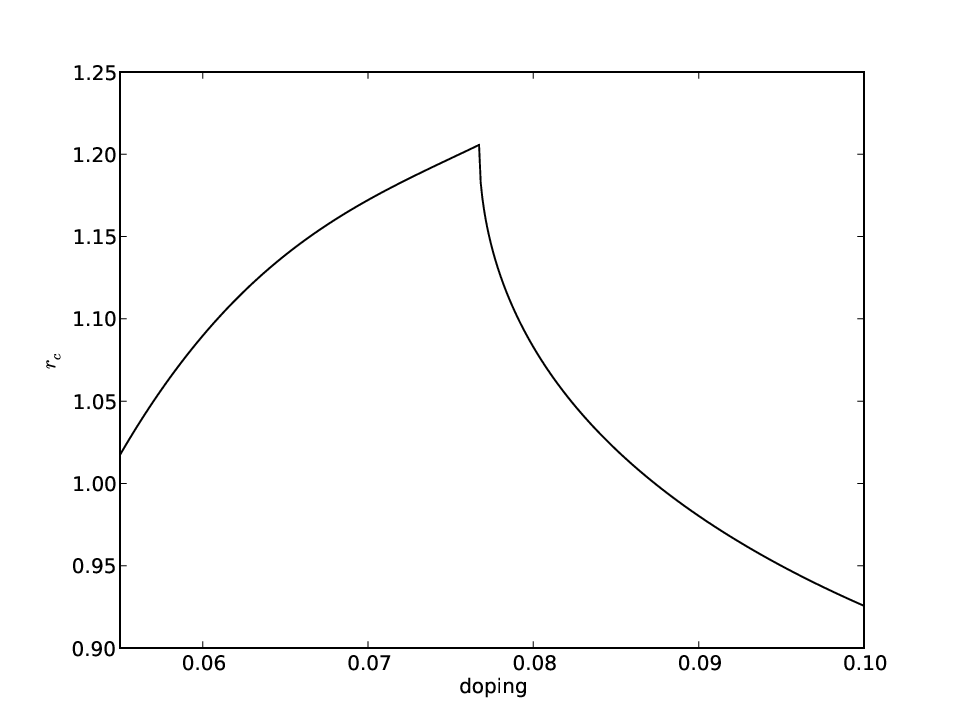
In real system, due to the more complicated shape of the electron and hole pockets, with increasing doping the pockets will experience cutting and touching several times after translating by in the momentum space. We have used a five-band model developed in Ref. [31] with all the orbitals on the Fe atoms, and calculated the mean field phase diagram close to the critical doping. The order parameter couple to the electrons at the Fermi surface as: . The mean field energy of electrons due to nonzero spin order parameter will renormalize in field theory Eq. 22, and hence the critical depends on the shape of the Fermi surface, which is tuned by doping. The critical is expected to be proportional to the critical pressure in the global phase diagram. as a function of doping is plotted in Fig. 6, and the shapes of the Fermi pockets at the critical doping is plotted in Fig. 7.

The quantum critical behavior discussed in this section is only applicable to small enough energy scale. First of all, the damping term always competes with a quadratic term in the Lagrangian, and at small enough energy scale the linear term dominates. If we assume the coupling between the spin order parameter and the electrons is of the same order as the effective spin interaction , the damping rate is linear with , while the quadratic term is . Therefore the frequency should be smaller than in order to apply the field theory Eq. 22. The value of has been calculated by LDA [19], and also measured with inelastic neutron scattering [20], and both approaches indicate that meV. is the Fermi energy of the Fermi pockets, which is of the order of meV. Therefore the frequency-linear damping term will dominate the the frequency quadratic term in the Lagrangian as long as meV.
The damping rate of order parameters is calculated assuming the Fermi surface can be linearly expanded close to the intersection point after translation in the momentum space, the criterion to apply this assumption depends on the details on the Fermi surface. In the particular situation under discussion, this crossover energy scale is meV in the undoped material, which is larger than the upper limit of 3meV we obtained previously. Therefore the ultraviolet cut-off of field theory Eq. 22 is estimated to be meV.
III III, three dimensional lattices
As mentioned in the introduction, compared with the 1111 materials, the 122 materials are much more isotropic, so we will treat this family of materials as a three dimensional problem. If after translation by the hole pockets intersect with the electron pockets, the zero temperature quantum transition is described a , transition with analogous Lagrangian as Eq. 14, which becomes a stable mean field transition. The finite temperature transition is described by two copies of coupled 3D O(3) transition. If the finite temperature transition is split into two transitions close to the quantum critical point, as observed in [11], one can estimate the size of the splitting close to the quantum critical point. These two transitions, as explained before, is driven by the only relevant perturbation at the coupled 3D O(3) transition, because the Ising order parameter is obtained by minimizing this term through Hubbard-Stratonovich transformation. The scaling dimension of at the 3D O(3) transition is , while at the , mean field fixed point has dimension . Therefore close to the quantum critical regime, to estimate the effect of one should use the renormalized value . The size of the splitting of the finite temperature transition close to the quantum critical point can be estimated as
| (36) |
is the exponent defined as at the 3D O(3) universality class. still scales with in terms of a universal law . The number can be estimated in a Heisenberg model on the square lattice as introduced in Ref. [14], the value is given by . However, model is not designed for describing a metallic phase, so the legitimacy of applying the model to Fe-pnictides is still under debate. In the finite temperature quantum critical regime, the specific heat, NMR relaxation rate scale as
| (37) |
The similar analysis also applies when the finite temperature transition is one single first order transition, which is the more common situation in 122 materials. One can estimate the jump of the lattice constant, and the jump of the SDW order parameter at the finite temperature first order transition close to the quantum critical point as
| (38) | |||||
| (40) |
is the lattice constant, which is linear with the Ising order parameter . is the critical exponent at the 3D O(3) transition defined as .
If under doping the hole pockets and electron pockets do not intersect (which depends on the details of direction dispersions), this transition becomes two copies of coupled , transition with three quartic terms , and :
| (41) | |||||
| (43) | |||||
| (45) | |||||
| (47) |
The coupled RG equation of the quartic terms are exactly the same as the one in Eq. 30, therefore this free energy is also subjected to an extremely weak run-away flow, which is negligible unless the length scale is large enough. Again, one can estimate the universal scaling behavior in the quantum critical regime contributed by the quantum critical modes:
| (48) |
IV IV, coupling to a soft lattice
Recent specific heat measurement on reveals two close but separate transitions at finite temperature, with a sharp peak at the SDW transition, and a discontinuity at the lattice distortion transition [11]. A discontinuity of specific heat is a signature of mean field transition, in contrast to the sharp peak of Wilson-Fisher fixed point in 3 dimensional space. The specific heat data suggest that the nature of the Ising nematic transition is strongly modified from the Wilson-Fisher fixed point, while SDW transition is unaffected. In the following we will attribute this difference to the lattice strain field fluctuations.
The SDW transition at finite temperature should belong to the 3D O(3) transition ignoring the lattice. The O(3) order parameter couples to the the lattice strain field with a quadratic term [34]:
| (49) |
which after integrating out the displacement vector generates a singular long range interaction between in the real space:
| (50) |
is a dimensionless function which depends on the direction of . The scaling dimension of is , and is the standard exponent at the 3D O(3) transition, which is greater than according to various types of numerical computations [33]. Therefore this long range interaction is irrelevant at the 3D O(3) transition, and by coupling to the strain field of the lattice, the SDW transition is unaffected. However, if the SDW has an Ising uniaxial anisotropy, the SDW transition becomes a 3D Ising transition with , and the strain field would lead to a relevant long range interaction.
However, since the symmetry of the Ising order parameter is the same as the shear strain of the lattice, the strain tensor will couple to the coarse grained Ising field as
| (51) |
is the displacement vector, The ellipses are all the elastic modulus terms. Notice that we have rotated the coordinates by 45 degree, since the true unit cell of the system is a two Iron unit cell. After integrating out the displacement vector , the effective free energy of gains a new singular term at small momentum:
| (52) |
is a function of spherical coordinates and defined as , but is independent of the magnitude of momentum . By tuning the uniform susceptibility , at some spherical angle of the space the minima of start to condense, we will call these minima as nodal points. These nodal points are isolated from each other on the two dimension unit sphere labelled by the solid angles , and are distributed symmetrically on the unit sphere according to the lattice symmetry transformation. Now suppose one nodal point of is located at , we rotate the direction along , and expand at this nodal point in terms of , the whole free energy can be written as
| (53) |
Notice that if is a nodal point, then has to be another nodal point. The naive power counting shows that effectively the spatial dimension of this field theory Eq. 53 is , and the scaling dimension of is . The quartic term takes an unusual form in the new momentum space of , but the straightforward power counting indicates that it is still an irrelevant operator. Therefore the strain tensor fluctuation effectively increases the dimension by two, which drives the transition a mean field transition.
Another way to formulating this effective 5 dimensional theory is that, close to the minimum , if the scaling dimension of is fixed to be 1, then effectively have scaling dimension 2. Therefore expanded at the minimum the quadratic part of the free energy of reads:
| (54) |
The total dimension is still 5, considering . All the other momentum dependent terms in the free energy are irrelevant.
The symmetry of the lattice allows multiple degenerate nodal points of function on the unit sphere labelled by solid angles. If the only nodal points are north and south poles , which is allowed by the tetragonal symmetry of the lattice, the theory becomes a precise 5 dimensional theory. However, the symmetry of the system also allows four stable degenerate nodal points on the equator, for instance at with . Close to nodal points , , while close to nodal points , . Therefore the scattering between these nodal points complicates the naive counting of the scaling dimensions, although is still valid. The transition in this case may still be a stable mean field transition, but more careful analysis of the loop diagrams is demanded to be certain. Let us denote the mode at and as and , and denote and modes as and , the expanded free energy reads
| (55) | |||||
| (57) | |||||
| (59) | |||||
| (61) | |||||
| (63) | |||||
| (65) |
The and terms describe the scattering between different nodal points. To see whether the mean field transition is stable, one can calculate the one-loop corrections to and , and none of the loops introduces nonperturbative divergence in the infrared limit. This analysis suggests that the Ising nematic transition is a mean field transition even with multiple nodal points of function on the equator.
V V, summaries and extensions
In this work we studied the global phase diagram of the magnetic order and lattice distortion of the Fe-pnictides superconductors. A two dimensional and three dimensional formalisms were used for 1111 and 122 materials respectively. The superconductivity was ignored so far in this material. If the quantum critical points discussed in this paper occur inside the superconducting phase, our results can be applied to the case when superconducting phase is suppressed. For instance, in 1111 materials, if a transverse magnetic field higher than is turned on, the field theory Eq. 6 and Eq. 22 become applicable. If the of the superconductor is lower than the ultraviolet cut-off of our field theory, the scaling behavior predicted in our work can be applied to the temperature between and the cut-off. Inside the superconducting phase, the nature of the transition may be changed. In 122 materials, the ARPES measurements on single crystals indicate that the fermi pockets are fully gapped in the superconducting phase [30], therefore the magnetic and nematic transitions are described by the , field theory Eq. 47, which is an extremely weak first order transition. In 1111 materials, although many experimental facts support a fully gapped fermi surface, wave pairing with nodal points is still favored by the Andreev reflection measurements [29, 28]. The nematic transition is the background of wave superconductor is studied in Ref. [21, 24, 23].
In most recently discovered 11 materials , the SDW and lattice distortion are both different from the 1111 and 122 materials [25]. The SDW state breaks the reflection symmetries about both line and axis there are two different Ising symmetries broken in the SDW state, the ground state manifold is . In this case, the classical and quantum phase diagrams are more interesting and richer, and since the order moments of the SDW in 11 materials are much larger than 1111 and 122 materials (about ), a lattice Heisenberg model with nearest neighbor, 2nd nearest neighbor, and 3rd nearest neighbor interactions () may be adequate in describing 11 materials, as was studied in Ref. [40].
Besides the quantum phase transitions studied in our current work, a quantum critical point is conjectured between the based and based materials [36], the field theory of this quantum critical point is analogous to Eq. 14. The formalism used in our work is also applicable to phase transitions in other strongly correlated materials, for instance the spin-dimer material , which under strong magnetic field develops long range XY order interpreted as condensation of spin triplet component [37]. This quantum critical point also has dynamical exponent , although the frequency linear term is from the Larmor precession induced by the magnetic field, instead of damping with particle-hole excitations. The frustration between the nearest neighbor layers in this material introduces an extra Ising symmetry between the even and odd layers besides the XY spin symmetry, therefore the quartic terms of this field theory are identical with Eq. 22. The RG equations of these quartic terms are much simpler than Eq. 30, because only the “ladder” like Feynman diagrams need to be taken into account [38]. We will study the material in detail in a future work [39].
Acknowledgements.
We thank Subir Sachdev and Qimiao Si for heplful discussions. We especially appreciate Bert Halperin for educating us about his early work on phase transitions on soft cubic lattice [34].References
- [2] Clarina de la Cruz, Q. Huang, J. W. Lynn, Jiying Li, W. Ratcliff II, J. L. Zarestky, H. A. Mook, G. F. Chen, J. L. Luo, N. L. Wang, Pengcheng Dai, Nature 453, 899 (2008).
- [3] Jun Zhao, Q. Huang, Clarina de la Cruz, Shiliang Li, J. W. Lynn, Y. Chen, M. A. Green, G. F. Chen, G. Li, Z. Li, J. L. Luo, N. L. Wang, Pengcheng Dai, Nature Materials 7, 953-959 (2008).
- [4] Q. Huang, Y. Qiu, Wei Bao, J.W. Lynn, M.A. Green, Y. Chen, T. Wu, G. Wu, X.H. Chen, arXiv:0806.2776 (2008).
- [5] C. Krellner, N. Caroca-Canales, A. Jesche, H. Rosner, A. Ormeci, C. Geibel, Phys. Rev. B 78, 100504(R) (2008).
- [6] J.-Q. Yan, A. Kreyssig, S. Nandi, N. Ni, S. L. Bud’ko, A. Kracher, R. J. McQueeney, R. W. McCallum, T. A. Lograsso, A. I. Goldman, P. C. Canfield, Phys. Rev. B. 78, 024516 (2008).
- [7] Jun Zhao, W. Ratcliff II, J. W. Lynn, G. F. Chen, J. L. Luo, N. L. Wang, Jiangping Hu, Pengcheng Dai, Phys. Rev. B 78, 140504(R) (2008).
- [8] A.I. Goldman, D.N. Argyriou, B. Ouladdiaf, T. Chatterji, A. Kreyssig, S. Nandi, N. Ni, S. L. Bud’ko, P.C. Canfield, R. J. McQueeney, Phys. Rev. B 78, 100506(R) (2008).
- [9] R. H. Liu, G. Wu, T. Wu, D. F. Fang, H. Chen, S. Y. Li, K. Liu, Y. L. Xie, X. F. Wang, R. L. Yang, L. Ding, C. He, D. L. Feng, X. H. Chen, Phys. Rev. Lett 101, 087001(2008).
- [10] Serena Margadonna, Yasuhiro Takabayashi, Martin T. McDonald, Michela Brunelli, G. Wu, R. H. Liu, X. H. Chen, Kosmas Prassides, arXiv:0806.3962 (2008).
- [11] Jiun-Haw Chu, James G. Analytis, Chris Kucharczyk, Ian R. Fisher, arXiv:0811.2463 (2008).
- [12] N. Ni, M. E. Tillman, J.-Q. Yan, A. Kracher, S. T. Hannahs, S. L. Bud’ko, P. C. Canfield, arXiv:0811.1767 (2008).
- [13] F.L. Ning, K. Ahilan, T. Imai, A. S. Sefat, R. Jin, M. A. McGuire, B. C. Sales, D. Mandrus, arXiv:0811.1617 (2008).
- [14] Qimiao Si, Elihu Abrahams, arXiv:0804.2480 (2008).
- [15] Lijun Zhu, Markus Garst, Achim Rosch, Qimiao Si, Phys. Rev. Lett, 91, 066404 (2003).
- [16] Cenke Xu, Markus Mueller, Subir Sachdev, Phys. Rev. B 78, 020501(R) (2008).
- [17] Chen Fang, Hong Yao, Wei-Feng Tsai, JiangPing Hu, Steven A. Kivelson, Phys. Rev. B 77 224509 (2008).
- [18] M. A. McGuire, A. D. Christianson, A. S. Sefat, B. C. Sales, M. D. Lumsden, R. Jin, E. A. Payzant, D. Mandrus, Y. Luan, V. Keppens, V. Varadarajan, J. W. Brill, R. P. Hermann, M. T. Sougrati, F. Grandjean, G. J. Long, Phys. Rev. 78, 094517 (2008).
- [19] Fengjie Ma, Zhongyi Lu, Tao Xiang, arXiv:0804.3370 (2008).
- [20] Jun Zhao, Dao-Xin Yao, Shiliang Li, Tao Hong, Y. Chen, S. Chang, W. Ratcliff II, J. W. Lynn, H. A. Mook, G. F. Chen, J. L. Luo, N. L. Wang, E. W. Carlson, Jiangping Hu, Pengcheng Dai, Phys. Rev. Lett 101, 167203 (2008).
- [21] Eun-Ah Kim, Michael J. Lawler, Paul Oreto, Subir Sachdev, Eduardo Fradkin, Steven A. Kivelson, Phys. Rev. B 77, 184514 (2008).
- [22] Kai Sun, Benjamin M. Fregoso, Michael J. Lawler, Eduardo Fradkin, Phys. Rev. B 78, 085124 (2008).
- [23] Cenke Xu, Yang Qi, Subir Sachdev, Phys. Rev. B 78, 134507 (2008).
- [24] Yejin Huh, Subir Sachdev, Phys. Rev. B 78, 064512 (2008).
- [25] Shiliang Li, Clarina de la Cruz, Q. Huang, Y. Chen, J. W. Lynn, Jiangping Hu, Yi-Lin Huang, Fong-chi Hsu, Kuo-Wei Yeh, Maw-Kuen Wu, Pengcheng Dai, arXiv:0811.0195 (2008).
- [26] H. Q. Yuan, J. Singleton, F. F. Balakirev, G. F. Chen, J. L. Luo, N. L. Wang, arXiv:0807.3137 (2008).
- [27] Fengjie Ma, Zhong-Yi Lu, Tao Xiang, arXiv:0806.3526 (2008).
- [28] Oded Millo, Itay Asulin, Ofer Yuli, Israel Felner, Zhi-An Ren, Xiao-Li Shen, Guang-Can Che, Zhong-Xian Zhao, Phys. Rev. B 78, 092505 (2008).
- [29] Yonglei Wang, Lei Shan, Lei Fang, Peng Cheng, Cong Ren, Hai-Hu Wen, arXiv:0806.1986 (2008).
- [30] H. Ding, P. Richard, K. Nakayama, T. Sugawara, T. Arakane, Y. Sekiba, A. Takayama, S. Souma, T. Sato, T. Takahashi, Z. Wang, X. Dai, Z. Fang, G. F. Chen, J. L. Luo, N. L. Wang, Europhysics Letters 83, 47001 (2008).
- [31] K. Kuroki, S. Onari, R. Arite, H. Usui, Y. Tanaka, H. Kontani, and H. Aoki, Phys. Rev. Lett. 101, 087004(2008)
- [32] Vadim Oganesyan, Steven Kivelson, Eduardo Fradkin, Phys. Rev. B 64, 195109 (2001).
- [33] Pasquale Calabrese, Andrea Pelissetto, Ettore Vicari, cond-mat/0306273, (2003).
- [34] D. Bergman and B. I. Halperin, Phys. Rev. B. 13, 2145 (1976).
- [35] J. A. Hertz, Phys. Rev. B 14, 1165 (1976).
- [36] Jianhui Dai, Qimiao Si, Jian-Xin Zhu, Elihu Abrahams, arXiv:0808.0305 (2008).
- [37] S. E. Sebastian, N. Harrison, C. D. Batista, L. Balicas, M. Jaime, P. A. Sharma, N. Kawashima, I. R. Fisher, Nature 441, 617 (2006).
- [38] Subir Sachdev, , Cambridge University Press, 1998.
- [39] Cenke Xu, in progress.
- [40] Chen Fang, B. Andrei Bernevig, Jiangping Hu, arXiv:0811.1294 (2008).