Twenty Digits of Some Integrals of the Prime Zeta Function

Richard J. Mathar URL: http://www.mpia-hd.mpg.de/˜mathar Address: Max-Planck Institute of Astronomy, Königstuhl 17, 69117 Heidelberg, Germany

Date: August 24, 2026

Abstract.

The double sum $\sum_{s\geq 1}\sum_{p}1/(p^{s}\log p^{s})=2.00666645\ldots$ over the inverse of the product of prime powers $p^{s}$ and their logarithms, is computed to 24 decimal digits. The sum covers all primes $p$ and all integer exponents $s\geq 1$ . The calculational strategy is adopted from Cohen’s work which basically looks at the fraction as the underivative of the Prime Zeta Function, and then evaluates the integral by numerical methods.

Key words and phrases:

Euler products, quasi-primitive sequences, Prime Zeta Function

2010 Mathematics Subject Classification

Primary 11Y60, 11M06; Secondary 11A41

1. Overview

Definition 1.

The constant in the focus of this work is the sum

(1)

C\equiv\sum_{s=1}^{\infty}\sum_{p}\frac{1}{p^{s}\log(p^{s})}

over all primitive prime powers $p^{s}$ of the prime numbers $p$ [15, 2.27.3][14, §2.2].

Remark 1.

The prime powers are represented by Sloane’s sequence A000961—we drop the leading term $p^{s}=1$ to avoid division by zero—. The constant $C$ and the contribution of $s=1$ are entry A137250 and A137245 [16].

The only aim of the work is to improve on the previous estimates $2.00<C<2.01$ [12] and $C>2.006$ [4].

The simple computational strategy is to accumulate the partial sums over $s$ in

(2)

C\equiv\sum_{s=1}^{\infty}\frac{1}{s}\sum_{p}\frac{1}{p^{s}\log p},

which converge at reasonable speed to an accuracy of $10^{-7}$ in $C$ after 20 terms or to an accuracy of $10^{-19}$ after 59 terms, for example.

2. Cohen’s Integral

The implementation is a shameless replica of Henri Cohen’s reduction of the double sum over exponents and primes to a series of integrals [8].

2.1. Logarithm-to-Integral Conversion

The logarithm of Euler’s formula for Riemann’s zeta function [3][19, 9.523.1]

(3)

\zeta(s)=\prod_{p}\frac{1}{1-p^{-s}}

(4)

\log\zeta(s)=-\sum_{p}\log(1-p^{-s}),

which turns with the Taylor expansion of the logarithm into [19, 9.523.2][23]

(5)

\log\zeta(s)=\sum_{k=1}^{\infty}\sum_{p}\frac{1}{kp^{ks}}.

Definition 2.

The Prime Zeta Function is [17, 27]

(6)

P(s)=\sum_{p}\frac{1}{p^{s}};\quad\Re s>1.

So the penultimate equation can be rephrased as

(7)

\log\zeta(s)=\sum_{k=1}^{\infty}\frac{1}{k}P(ks).

The Möbius inversion of this formula reads [2, (9b)][10, §17.1.3][29]

(8)

P(s)=\sum_{k=1}^{\infty}\frac{\mu(k)}{k}\log\zeta(ks).

First integrals of terms in (6) are [9, 565.1.]

(9)

\int_{s}^{\infty}\frac{1}{p^{t}}dt=\frac{1}{p^{s}\log p},\quad s>1,

so integration of (8) using (6) gives

(10)

\int_{s}^{\infty}\sum_{p}\frac{dt}{p^{t}}=\sum_{p}\frac{1}{p^{s}\log p}=\sum_{k=1}^{\infty}\frac{\mu(k)}{k}\int_{s}^{\infty}\log\zeta(kt)dt=\sum_{k=1}^{\infty}\frac{\mu(k)}{k^{2}}\int_{ks}^{\infty}\log\zeta(t)dt.

Definition 3.

Cohen’s integral is

(11)

I_{n}(m)\equiv\frac{1}{n!}\int_{m}^{\infty}(t-m)^{n}\log\zeta(t)dt,\quad n=0,1,2,\ldots

over the logarithm of Riemann’s zeta function with variable integer lower limit [8].

Insertion into (10) outlines the strategy to evaluate (2),

(12)

\sum_{p}\frac{1}{p^{s}\log p}=\sum_{k=1}^{\infty}\frac{\mu(k)}{k^{2}}I_{0}(ks).

2.2. Transition to the Dirichlet Eta Function

For $I_{0}(1)$ , the pole of $\zeta(t)$ at $t=1$ can be isolated by handling the singularity via the smooth function [1, 23.2.19][30, p 267]

(13)

\eta(s)\equiv(1-2^{1-s})\zeta(s).

For lower limits of the integral larger than one, this recipe is not needed; we stick to it to present a shorter, simpler program.

Remark 2.

The finite value at $s=1$ is [15][19, 0.232.1,1.511]

(14)

\eta(1)=\log 2.

This follows also from the residuum of $\mathop{\mathrm{Res}}\nolimits\zeta(s)_{\mid s=1}=1$ in conjunction with the Taylor expansion $1-2^{1-s}=-\sum_{l=1}^{\infty}\frac{(-\log 2)^{l}}{l!}(s-1)^{l}=(s-1)\log 2-\frac{\log^{2}2}{2}(s-1)^{2}+O((s-1)^{3})$ . If we introduce Stieltjes constants $\gamma_{j}$ [5, 6, 7],

(15)

\zeta(s)=\frac{1}{s-1}+\gamma-\gamma_{1}(s-1)+\frac{\gamma_{2}}{2}(s-1)^{2}+\cdots,

the Taylor series of $\eta$ near $s=1$ becomes

(16)

\eta(s)=\log 2+\log 2\left(\gamma-\frac{\log 2}{2}\right)(s-1)-\log 2\left(\gamma_{1}+\gamma\frac{\log 2}{2}-\frac{\log^{2}2}{6}\right)(s-1)^{2}+\ldots.

The integrated logarithm of (13) is

(17)

\int_{m}^{\infty}ds\log\eta(s)=\int_{m}^{\infty}ds\log(1-2^{1-s})+\int_{m}^{\infty}ds\log\zeta(s).

One term is a dilogarithm [18, 20, 22, 26],

(18)

\int_{m}^{\infty}\log\left(1-2^{1-s}\right)ds=\int_{1-2^{1-m}}^{1}\frac{\log x}{\log 2(1-x)}dx\\ =-\frac{1}{\log 2}\mathop{\mathrm{Li}}\nolimits_{2}\left(\frac{1}{2^{m-1}}\right).

Remark 3.

Special values at $m=1$ and $m=2$ are $\mathop{\mathrm{Li}}\nolimits_{2}(1)=\pi^{2}/6$ and $\mathop{\mathrm{Li}}\nolimits_{2}(1/2)=\pi^{2}/12-\frac{1}{2}\log^{2}(2)$ [25]; see the constants A013661 and A076788 in the On-Line Encyclopedia of Integer Sequences [16]. An accurate representation of $\pi^{2}/(12\log 2)$ is entry A100199. $\eta(1)=\log 2$ is A002162, $\gamma$ is A001620, $\eta^{\prime}(1)=\log 2(\gamma-\log 2/2)$ is A091812, and $-\gamma_{1}$ is A082633.

This moulds (17) into

(19)

I_{0}(m)=\int_{m}^{\infty}ds\log\eta(s)+\frac{1}{\log 2}\mathop{\mathrm{Li}}\nolimits_{2}\left(\frac{1}{2^{m-1}}\right).

2.3. Numerical Implementation

The variable substitution

(20)

u=1-\frac{m}{s};\quad s=\frac{m}{1-u};\quad ds=\frac{m}{(1-u)^{2}}du

maps the interval $m\leq s<\infty$ onto the interval $0\leq u\leq 1$ .

Remark 4.

Alternative substitutions like $u=1/m-m/s^{2}$ or $u=1-2^{-s}$ also map the half-infinite $s$ -interval to a finite $u$ -interval. They have the advantage of more evenly balanced integral kernels, but the disadvantage of infinite slopes at one end of the $u$ -interval.

Wynn’s $\epsilon$ -algorithm [31, 24] is applied to numerical values gathered by the trapezoidal rule to evaluate the $\eta$ -integral in (19),

(21)

\int_{m}^{\infty}ds\log\eta(s)=m\int_{0}^{1}\frac{\log\eta\left(\frac{m}{1-u}\right)}{(1-u)^{2}}du.

Remark 5.

Because $\log\zeta(s)\approx 2^{-s}$ at $s>10$ , $I_{0}(m)\approx 1/(2^{m}\log 2)$ as $m\to\infty$ . This functional dependence leads to an almost straight line on the semi-logarithmic plot in Fig. 2. So the first neglected term in (2) is a good estimator to the error in the partial sums.

Refer to caption — Figure 1. The functions $(m\log\eta)/(1-u)^{2}<0$ and $(m\log\zeta)/(1-u)^{2}>0$ arising in the integral kernels through the substitution (20).

Figure 2. The functions

I_{0}(s)

and

\sum_{p}\frac{1}{p^{s}\log p}

fall of exponentially as a function of their argument

s

, and are not distinguishable in this common plot.

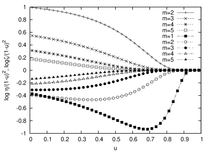
2.4. Intermediate Results

The following table shows $s$ and $I_{0}(s)$ in the left double column, $s$ and $\sum_{p}1/(p^{s}\log p)$ in the right double column, last digits rounded:

  1 1.797569958628739407930251e+00    1 1.636616323351260868569658e+00
  2 5.365269459211771009617190e-01    2 5.077821878591993187743751e-01
  3 2.275044530363196437654595e-01    3 2.212033403969814969599433e-01
  4 1.041502253168599126451383e-01    4 1.026654782331571962664758e-01
  5 4.942465209576037094607771e-02    5 4.906357474830439568004180e-02
  6 2.392429939526549813915300e-02    6 2.383519825459824737569112e-02
  7 1.171800374394507398697301e-02    7 1.169586557789515115400634e-02
  8 5.781462903507255601662420e-03    8 5.775944595316604352784204e-03
  9 2.865717415930253367688719e-03    9 2.864339771659922115926198e-03
 10 1.424706500149304604154559e-03   10 1.424362320209387639441021e-03
 11 7.096782687818267364308355e-04   11 7.095922515383712411613441e-04
 12 3.539573278954885950994965e-04   12 3.539358269254206683875757e-04
 13 1.766870488681893665136623e-04   13 1.766816740292220402778692e-04
 14 8.824687187128450251937842e-05   14 8.824552821042831521626792e-05
 15 4.409135113515804839684079e-05   15 4.409101522588177584140913e-05
 16 2.203501275340515891846297e-05   16 2.203492877680910955374197e-05
 17 1.101395992552518507579192e-05   17 1.101393893146441713313451e-05
 18 5.505799725855358158700238e-06   18 5.505794477350959773416061e-06
 19 2.752506920732716039062161e-06   19 2.752505608607939317868454e-06
 20 1.376122595515799546777009e-06   20 1.376122267484767801052807e-06
 21 6.880177047831559600925881e-07   21 6.880176227754180030145763e-07
 22 3.439943284950306802000172e-07   22 3.439943079930986522426868e-07
 23 1.719923247093458602614288e-07   23 1.719923195838631569242761e-07
 24 8.599454961284003932811501e-08   24 8.599454833146940100459182e-08
 25 4.299673733467609442174442e-08   25 4.299673701433343948018079e-08
 26 2.149818953720244919068455e-08   26 2.149818945711678602970514e-08
 27 1.074903506531325106214723e-08   27 1.074903504529183534309235e-08
 28 5.374497633245768258586266e-09   28 5.374497628240414337653354e-09
 29 2.687242183906380835200363e-09   29 2.687242182655042356063437e-09
 30 1.343618881152634756065114e-09   30 1.343618880839800136417081e-09
 31 6.718087036690018174171263e-10   31 6.718087035907931625220498e-10
 32 3.359041062052731307704559e-10   32 3.359041061857209670487929e-10
 33 1.679519712278619904984955e-10   33 1.679519712229739495683419e-10
 34 8.397595832274787450826827e-11   34 8.397595832152586427576250e-11
 35 4.198797006441494468678066e-11   35 4.198797006410944212865828e-11
 36 2.099398199991330939924248e-11   36 2.099398199983693375971239e-11
 37 1.049698998919830689452100e-11   37 1.049698998917921298463855e-11
 38 5.248494657681297045976310e-12   38 5.248494657676523568505703e-12
 39 2.624247216535094520600355e-12   39 2.624247216533901151232704e-12
 40 1.312123570832462108601650e-12   40 1.312123570832163766259737e-12
 41 6.560617729378942125931467e-13   41 6.560617729378196270076685e-13
 42 3.280308823095077105921359e-13   42 3.280308823094890641957663e-13
 43 1.640154397682756111408190e-13   43 1.640154397682709495417266e-13
 44 8.200771942197877942789073e-14   44 8.200771942197761402811764e-14
 45 4.100385955693647813828150e-14   45 4.100385955693618678833822e-14
 46 2.050192972711729282745366e-14   46 2.050192972711721998996784e-14
 47 1.025096484644167040382940e-14   47 1.025096484644165219445795e-14
 48 5.125482417515178049571403e-15   48 5.125482417515173497228539e-15
 49 2.562741206855703686734819e-15   49 2.562741206855702548649103e-15
 50 1.281370602793890158864587e-15   50 1.281370602793889874343158e-15
 51 6.406853011856245416428711e-16   51 6.406853011856244705125138e-16
 52 3.203426505223720974861043e-16   52 3.203426505223720797035150e-16
 53 1.601713252377059924465468e-16   53 1.601713252377059880008995e-16
 54 8.008566261102631116158675e-17   54 8.008566261102631005017492e-17
 55 4.004283130290426065285105e-17   55 4.004283130290426037499809e-17
 56 2.002141565058249870693295e-17   56 2.002141565058249863746971e-17
 57 1.001070782500137215275764e-17   57 1.001070782500137213539183e-17
 58 5.005353912404060344256377e-18   58 5.005353912404060339914924e-18
 59 2.502676956169821595115832e-18   59 2.502676956169821594030469e-18
 60 1.251338478074174605310912e-18   60 1.251338478074174605039571e-18
 61 6.256692390335085719290662e-19   61 6.256692390335085718612310e-19
 62 3.128346195155613757280562e-19   62 3.128346195155613757110974e-19
 63 1.564173097573830511199490e-19   63 1.564173097573830511157093e-19
 64 7.820865487855897997896814e-20   64 7.820865487855897997790822e-20
 65 3.910432743923530812923694e-20   65 3.910432743923530812897196e-20
 66 1.955216371960292677789151e-20   66 1.955216371960292677782526e-20
 67 9.776081859796554293375620e-21   67 9.776081859796554293359059e-21
 68 4.888040929896640781499146e-21   68 4.888040929896640781495005e-21
 69 2.444020464947774935687030e-21   69 2.444020464947774935685995e-21
 70 1.222010232473705649489420e-21   70 1.222010232473705649489161e-21
 71 6.110051162367922186267000e-22   71 6.110051162367922186266353e-22
 72 3.055025581183759072740187e-22   72 3.055025581183759072740025e-22
 73 1.527512790591812196239003e-22   73 1.527512790591812196238962e-22
 74 7.637563952958836514091412e-23   74 7.637563952958836514091310e-23
 75 3.818781976479343434677847e-23   75 3.818781976479343434677822e-23
 76 1.909390988239646776549639e-23   76 1.909390988239646776549633e-23
 77 9.546954941198150746783920e-24   77 9.546954941198150746783904e-24
 78 4.773477470599047661403870e-24   78 4.773477470599047661403866e-24
 79 2.386738735299514593372572e-24   79 2.386738735299514593372571e-24
 80 1.193369367649754217576498e-24   80 1.193369367649754217576498e-24

At large $s$ , the two values equalize because the first term at $k=1$ dominates the sum at the right hand side of (12). Cohen reported the first two rows [8]. Erdős and Zhang published an upper bound of $\sum_{p}1/(p\log p)$ [11]; a proof of convergence had been given earlier [13].

The rightmost column $P^{L}(s,1)$ is an aid to computation of the more general

(22)

P^{L}(s,a)\equiv\sum_{p}\frac{1}{(a-1+p)^{s}\log p}=\sum_{l=0}^{\infty}\binom{s+l-1}{s-1}(1-a)^{l}P^{L}(l+s,1).

The $l$ -series converges for $a=0$ and $a=2$ . Larger $a$ are then reached recursively with the alternating geometric series

(23)

P^{L}(s,a+1)=\sum_{p}\frac{1}{(a-1+p)^{s}\left(1+\frac{1}{a-1+p}\right)^{s}\log p}=\sum_{l=0}^{\infty}\binom{s+l-1}{s-1}(-1)^{l}P^{L}(s+l,a).

This yields the following short table with double columns of $s$ , $a$ and $P^{L}(s,a)$ each:

 1  0 2.564343220686309193e+00       4  2 2.200937333087681441e-02
 2  0 1.735535173734295407e+00       5  2 6.924273989916642133e-03
 3  0 1.569430040669505312e+00       6  2 2.216719348246691407e-03
 4  0 1.502480490856796843e+00       7  2 7.177059901294852453e-04
 5  0 1.471819234100400691e+00       8  2 2.341804937450834077e-04
 6  0 1.457080819283874067e+00       9  2 7.683437427098209717e-05
 7  0 1.449846098516752367e+00      10  2 2.531100154045370884e-05
 8  0 1.446260454845751749e+00      11  2 8.362846790350413196e-06
 9  0 1.444475273576531254e+00      12  2 2.769232699593665178e-06
10  0 1.443584547482253809e+00      13  2 9.185072149314254133e-07
11  0 1.443139643195342866e+00      14  2 3.050306451883795961e-07
12  0 1.442917304533643634e+00      15  2 1.013929603798279887e-07
13  0 1.442806163373811902e+00      16  2 3.372678630308857437e-08
14  0 1.442750599803600762e+00      17  2 1.122456404716334707e-08
15  0 1.442722819765431096e+00      18  2 3.737099942191877583e-09
16  0 1.442708930182166938e+00      19  2 1.244595144792613520e-09
17  0 1.442701985499337981e+00      20  2 4.145889249942980892e-10
18  0 1.442698513185098959e+00       1  3 1.083884561790478549e+00
19  0 1.442696777034769093e+00       2  3 1.539997501094314544e-01
20  0 1.442695908961300868e+00       3  3 3.279427700685188571e-02
 1  2 1.280433764453964036e+00       4  3 7.457583410785408360e-03
 2  2 2.518771844123868571e-01       5  3 1.747751882461897344e-03
 3  2 7.208846839108258174e-02

In the left column of this table we observe $\lim_{s\to\infty}P^{L}(s,0)=1/\log(2)\approx 1.44\ldots$ .

3. Higher Powers of The Logarithms

3.1. Quadratic

Repeated integration in the spirit of (2) generates higher powers of the logarithm in the denominator of the prime sums:

(24)

\int_{s}^{\infty}\frac{1}{p^{u}\log p}du=\frac{1}{p^{s}\log^{2}p}=\int_{s}^{\infty}du\int_{u}^{\infty}dt\frac{1}{p^{t}},

which integrates an infinite triangular region which extends right from $t=u$ and upwards from the diagonal $u\geq s$ . Interchange of the order of the two integrations contracts it to a single integral:

(25)

\sum_{p}\frac{1}{p^{s}\log^{2}p}=\int_{s}^{\infty}du\int_{u}^{\infty}dtP(t)=\int_{t=s}^{\infty}dt\int_{u=s}^{t}dsP(t)\\ =\int_{t=s}^{\infty}dt(t-s)\sum_{k=1}^{\infty}\frac{\mu(k)}{k}\log\zeta(kt)=\int_{x=sk}^{\infty}dx(x-sk)\sum_{k=1}^{\infty}\frac{\mu(k)}{k^{3}}\log\zeta(x)\\ =\sum_{k=1}^{\infty}\frac{\mu(k)}{k^{3}}I_{1}(sk).

As before it is numerically advantageous to employ the $\eta$ -function (13) in the integral kernel of $I_{1}$ for small $m$ :

(26)

\int_{m}^{\infty}dt(t-m)\log\eta(t)=\int_{m}^{\infty}dt(t-m)\log(1-2^{1-t})+\int_{m}^{\infty}dt(t-m)\log\zeta(t).

The contribution from $1-2^{1-t}$ becomes a mix of well-converging polylogarithmic constants. We substitute

(27)

x=1-2^{1-t},\quad t=1-\log(1-x)/\log 2,\quad dt=\frac{dx}{(1-x)\log 2}

to approach standard integrals over products of logarithms:

(28)

\int_{m}^{\infty}dt(t-m)\log(1-2^{1-t})\\ =\frac{1}{\log 2}\int_{1-2^{1-m}}^{1}\frac{dx}{1-x}[1-\frac{\log(1-x)}{\log 2}-m]\log x\\ =\frac{1-m}{\log 2}\int_{0}^{2^{1-m}}\frac{du}{u}\log(1-u)-\frac{1}{\log^{2}2}\int_{0}^{2^{1-m}}\frac{du}{u}\log(u)\log(1-u)\\ =\frac{1-m}{\log 2}l_{0,1}(2^{1-m})-\frac{1}{\log^{2}2}l_{1,1}(2^{1-m}).

The $l$ -integrals are defined by the powers of the two logarithms in the kernel, and discussed in the appendix for the upper limits of interest:

Definition 4.

(Polylogarithmic Constants)

(29)

l_{i,j}(x)\equiv\int_{0}^{x}\log^{i}(u)\log^{j}(1-u)\frac{du}{u}.

The values of $I_{1}$ in (25) are eventually computed for $m=1$ and $m=2$ via

(30)

I_{1}(m)=\int_{m}^{\infty}(s-m)\log\eta(s)ds-\int_{m}^{\infty}(s-m)\log(1-2^{1-s})ds

and numerical integration of the first term on the right hand side. The important results are those for small $s$ where direct summation over the primes suffers from slow convergence [16, A319231,A319232]:

(31)	$\displaystyle\sum_{p}\frac{1}{p\log^{2}p}$	$\displaystyle\approx$	$\displaystyle 1.520970439939500\ldots$
(32)	$\displaystyle\sum_{p}\frac{1}{p^{2}\log^{2}p}$	$\displaystyle\approx$	$\displaystyle 0.637056184074676\ldots$
(33)	$\displaystyle\sum_{p}\frac{1}{p^{3}\log^{2}p}$	$\displaystyle\approx$	$\displaystyle 0.2949791653099842\ldots$

3.2. Cubic

Integrating (25) once more lifts the square to a cube in the denominator:

(34)

\sum_{p}\frac{1}{p^{s}\log^{3}p}=\int_{s}^{\infty}du\sum_{p}\frac{1}{p^{u}\log^{2}p}\\ =\int_{s}^{\infty}du\int_{t=u}^{\infty}dt(t-u)\sum_{k=1}^{\infty}\frac{\mu(k)}{k}\log\zeta(kt)\\ =\int_{t=s}^{\infty}dt\int_{u=s}^{t}du(t-u)\sum_{k=1}^{\infty}\frac{\mu(k)}{k}\log\zeta(kt)\\ =\frac{1}{2}\int_{s}^{\infty}dt(t-s)^{2}\sum_{k=1}^{\infty}\frac{\mu(k)}{k}\log\zeta(kt)=\frac{1}{2}\int_{ks}^{\infty}dx(x-ks)^{2}\sum_{k=1}^{\infty}\frac{\mu(k)}{k^{4}}\log\zeta(x)\\ =\sum_{k=1}^{\infty}\frac{\mu(k)}{k^{4}}I_{2}(sk).

(35)

\sum_{p}\frac{1}{p^{s}\log^{n}p}=\sum_{k=1}^{\infty}\frac{\mu(k)}{k^{n+1}}I_{n-1}(sk),\quad n=1,2,3,\ldots.

Similar to (30) we defer the $\zeta$ -function to the $\eta$ -function for small $m$ :

(36)

I_{2}(m)=\frac{1}{2}\int_{s=m}^{\infty}(s-m)^{2}\log\eta(s)ds-\frac{1}{2}\int_{s=m}^{\infty}(s-m)^{2}\log(1-2^{2-m})ds.

The second term is sliced with (27) as

(37)

\frac{1}{2}\int_{s=m}^{\infty}(s-m)^{2}\log(1-2^{1-m})ds=\frac{1}{2\log 2}\int_{x=1-2^{1-m}}^{1}\left[1-\frac{\log(1-x)}{\log 2}-m\right]^{2}\log x\frac{dx}{(1-x)}\\ =\frac{1}{2\log 2}\int_{u=0}^{2^{1-m}}[1-\frac{\log(u)}{\log 2}-m]^{2}\log(1-u)\frac{du}{u}\\ =\frac{(1-m)^{2}}{2\log 2}\int_{u=0}^{2^{1-m}}\log(1-u)\frac{du}{u}-\frac{1-m}{\log^{2}2}\int_{u=0}^{2^{1-m}}\log u\log(1-u)\frac{du}{u}+\frac{1}{2\log^{3}2}\int_{u=0}^{2^{1-m}}\log^{2}u\log(1-u)\frac{du}{u}\\ =\frac{(1-m)^{2}}{2\log 2}l_{0,1}(2^{1-m})-\frac{1-m}{\log^{2}2}l_{1,1}(2^{1-m})+\frac{1}{2\log^{3}2}l_{2,1}(2^{1-m}),

such that for $m=1$ and $m=2$ the $l_{i,j}$ can be taken from the appendix.

(38)	$\displaystyle\sum_{p}\frac{1}{p\log^{3}p}$	$\displaystyle\approx$	$\displaystyle 1.8461474193664495\ldots$
(39)	$\displaystyle\sum_{p}\frac{1}{p^{2}\log^{3}p}$	$\displaystyle\approx$	$\displaystyle 0.848270491703549\ldots$
(40)	$\displaystyle\sum_{p}\frac{1}{p^{3}\log^{3}p}$	$\displaystyle\approx$	$\displaystyle 0.405696596756787\ldots$

4. Summary

We obtained the constant

(41)

C=2.00666645283106875643229\ldots

by a rather basic numerical approach to Cohen’s integral over the logarithm of the Prime Zeta Function. A table of $\sum_{p}1/(p^{s}\log p)$ was generated for $1\leq s\leq 80$ and a table of $\sum_{p}1/[(p\pm 1)^{s}\log p]$ for $1\leq s\leq 20$ .

Appendix A Polylogarithm Constants

We gather the values of $l_{i,j}(x)$ that emerge in the main text while evaluating $I_{j}$ for $j=0,1$ and 2 and $m=1$ or 2. If $j=0$ the integrals are elementary [9, 616.1]:

(42)

\int\log^{i}(u)\frac{du}{u}=\frac{\log^{i+1}(u)}{i+1}.

If $j=x=1$ , the $l_{i,1}(1)$ are essentially $\zeta(i+2)$ -values: [28, 21]

(43)

l_{1,1}(1)=\int_{0}^{1}\frac{du}{u}\log(u)\log(1-u)=\zeta(3);

(44)

l_{2,1}(1)=\int_{0}^{1}\frac{du}{u}\log^{2}(u)\log(1-u)=-2\zeta(4)=-\frac{\pi^{4}}{45}.

If $x=1/2$ we have [19, 4.291.3]

(45)

l_{0,1}(1/2)=\int_{0}^{\frac{1}{2}}\frac{du}{u}\log(1-u)=\frac{1}{2}\log^{2}(2)-\frac{\pi^{2}}{12}.

A particular case of [25, A.3.5(8)]

(46)

l_{1,1}(x)=-\log(x)\mathop{\mathrm{Li}}\nolimits_{2}(x)+\mathop{\mathrm{Li}}\nolimits_{3}(x).

in conjunction with [25, A.2.6.(3)][16, A099217]

(47)

\mathop{\mathrm{Li}}\nolimits_{3}(1/2)=\frac{7}{8}\zeta(3)-\frac{\pi^{2}}{12}\log 2+\frac{1}{6}\log^{3}(2)\approx 0.537213193608\ldots

is [25, A2.1.(4), A2.6(3)]

(48)

l_{1,1}(1/2)=-\frac{1}{3}\log^{3}(2)+\frac{7}{8}\zeta(3)\approx 0.9407915729350018398184\ldots

The indefinite integral [25, A3.5.(10)]

(49)

l_{2,1}(x)=-2\mathop{\mathrm{Li}}\nolimits_{4}(x)+2\log(x)\mathop{\mathrm{Li}}\nolimits_{3}(x)-\log^{2}(x)\mathop{\mathrm{Li}}\nolimits_{2}(x)

generates

(50)

l_{2,1}(1/2)=-2\mathop{\mathrm{Li}}\nolimits_{4}(1/2)-2\log(2)\mathop{\mathrm{Li}}\nolimits_{3}(1/2)-\log^{2}(2)\mathop{\mathrm{Li}}\nolimits_{2}(1/2)\\ \approx-2.059432960131268548157225796\ldots

where [16, A099218]

(51)

2\mathop{\mathrm{Li}}\nolimits_{4}(1/2)={}_{5}F_{4}(1,1,1,1,1;2,2,2,2;1/2)\approx 1.034958123347798772\ldots

References

[1] Milton Abramowitz and Irene A. Stegun (eds.), Handbook of mathematical functions, 9th ed., Dover Publications, New York, 1972. MR 0167642
[2] E. A. Bender and J. R. Goldman, On the applications of Mobius inversion in combinatorial analysis, Amer. Math. Monthly 82 (1975), no. 8, 789–803. MR 0376360
[3] Jonathan Michael Borwein, David M. Bradley, and Richard E. Crandall, Computational strategies for the Riemann Zeta Function, J. Comput. Appl. Math. 121 (2000), 247–296. MR 1780051
[4] D. A. Clark, An upper bound of $\sum 1/(a_{i}\log a_{i})$ for quasi-primitive sequences, Comp. Math. Appl. 35 (1998), no. 4, 105–109. MR 1604728
[5] Mark W. Coffey, New results on the Stieltjes constants: Asymptotic and exact evaluations, J. Math. Anal. Appl. 317 (2006), 603–612. MR 2209581
[6] by same author, New summation relations for the Stieltjes constants, Proc. Roy. Soc. A: Math., Phys. &Eng. 462 (2006), no. 2073, 2563–2573. MR 2253550
[7] by same author, Series of zeta values, the Stieltjes constants, and a sum $S_{\gamma}(n)$ , arXiv:math-ph/0706.0345 (2007).
[8] Henri Cohen, High precision computation of Hardy-Littlewood constants, 1998, http://www.math.u-bordeaux.fr/˜cohen/hardylw.dvi.
[9] Herbert Bristol Dwight, Tables of integrals and other mathematical data, 3rd ed., Macmillan, New York, 1957. MR 0129577
[10] Arthur Erdélyi, Wilhelm Magnus, Fritz Oberhettinger, and Francesco G. Tricomi (eds.), Higher transcendental functions, vol. 3, McGraw-Hill, New York,London, 1953. MR 0066496
[11] P. Erdős and Zhenxiang Zhang, Upper bound of $\sum 1/(a_{i}\log a_{i})$ for primitive sequences, Proc. Am. Math. Soc. 117 (1993), no. 4, 891–895. MR 1116257
[12] by same author, Upper bound of $\sum 1/(a_{i}\log a_{i})$ for quasi-primitive sequences, Comp. Math. Appl. 26 (1993), no. 3, 1–5. MR 1221192
[13] Paul Erdős, Note on sequences of integers no one of which is divisible by any other, J. Lond. Math. Soc. 1–10 (1935), no. 38, 126–128. MR 1574239
[14] Steven Finch, Errata and addenda to “Mathematical Constants”, 22 July 2008.
[15] Steven R. Finch, Mathematical constants, Encyclopedia of Mathematics and its Applications, no. 94, Cambridge University Press, Cambridge, 2003. MR 2003519
[16] OEIS Foundation Inc., The On-Line Encyclopedia Of Integer Sequences, (2018), http://oeis.org/. MR 1992789
[17] Carl-Erik Fröberg, On the prime zeta function, BIT 8 (1968), no. 3, 187–202. MR 0236123
[18] Edward S. Ginsberg and Dorothy Zaborowski, Algorithm 490: The dilogarithm function of a real argument, Comm. ACM 18 (1975), no. 4, 200–202.
[19] I. Gradstein and I. Ryshik, Summen-, Produkt- und Integraltafeln, 1st ed., Harri Deutsch, Thun, 1981. MR 0671418
[20] Anatol N. Kirillov, Dilogarithm identities, Prog. Theor. Phys. Suppl. 118 (1995), 61–142.
[21] K. S. Kölbig, Closed expressions for $\int_{0}^{1}t^{-1}\log^{n-1}t\log^{p}(1-t)dt$ , Math. Comp. 39 (1982), no. 160, 647–654. MR 0669656
[22] K. S. Kölbig, J. A. Mignaco, and E. Remiddi, On Nielsen’s generalized polylogarithms and their numerical calculation, BIT Numerical Mathematics 10 (1970), no. 1, 38–74. MR 0285750
[23] Peter Gustav Lejeune-Dirichlet, Démonstration de cette proposition: Toute progression arithmétique dont le premier terme et la raison sont des entiers sans diviseur commun contient une infinité de nombres premiers, J. Math. Pures et Appl. 4 (1839), 393–422.
[24] David Levin and Avram Sidi, Two new classes of nonlinear transformations for accelerating the convergence of integrals and series, Appl. Math. Comp. 9 (1981), no. 3, 175–215. MR 0650681
[25] Leonard Lewin, Polylogarithms and associated functions, North Holland, 1981. MR 0618278
[26] J. H. Loxton, Special values of the dilogarithm function, Acta Arithm. 43 (1984), no. 2, 155–166. MR 0736728
[27] Richard J. Mathar, Series of reciprocal powers of $k$ -almost primes, arXiv:0803.0900 [math.NT] (2008).
[28] George Rutledge and R. D. Douglas, Table of definite integrals, Am. Math. Monthly 45 (1938), no. 8, 525–530. MR 1524383
[29] Pascal Sebah and Xavier Gourdon, Constants from number theory, 2001, http://numbers.computation.free.fr/Constants/constants.html.
[30] Edmund T. Whittaker and George Neville Watson, A course of modern analysis, 4 ed., Cambridge University Press, Cambridge, 1996. MR 1424469
[31] P. Wynn, On a device for computing the $e_{m}(s_{n})$ transformation, Math. Tabl. Aids Comput. 10 (1956), no. 54, 91–96. MR 0084056