Gromov-Witten Invariants of Toric Calabi-Yau Threefolds
Abstract.
Based on the large duality relating topological string theory on Calabi-Yau 3-folds and Chern-Simons theory on 3-manifolds, M. Aganagic, A. Klemm, M. Mariño and C. Vafa proposed the topological vertex, an algorithm on computing Gromov-Witten invariants in all genera of any non-singular toric Calabi-Yau 3-fold. In this expository article, we describe the mathematical theory of the topological vertex developed by J. Li, K. Liu, J. Zhou, and the author.
Key words and phrases:
topological vertex, Gromov-Witten invariants, Calabi-Yau threefolds2000 Mathematics Subject Classification
14N351. Gromov-Witten invariants of Calabi-Yau 3-folds
1.1. Symplectic and algebraic Gromov-Witten invariants
We start with a general setting. Let be a compact Kähler manifold, where is the Kähler form, and is the complex structure. For our purpose, we may assume that is a projective manifold, i.e., a compact complex submanifold of some complex projective space , and is the restriction of the Fubini-Study Kähler form on . In this case, one may work in complex algebraic geometry.
Intuitively, symplectic Gromov-Witten invariants count parametrized holomorphic curves in . When is projective, algebraic Gromov-Witten invariants count parametrized complex algebraic curves in , and should coincide with symplectic Gromov-Witten invariants.
1.2. Moduli space of stable maps
Gromov-Witten invariants can be viewed as intersection numbers on moduli spaces of parametrized holomorphic (complex algebraic) curves in . Let be the moduli space of holomorphic maps (morphisms) , where is a compact Riemann surface (smooth complex algebraic curve) of genus , and . We call the degree of the map. Two maps are equivalent if they differ by an automorphism of the domain .
To do intersection theory, we should compactify . The standard compactification in Gromov-Witten theory is , the Kontsevich’s moduli space of stable maps of genus , degree [26], where the domain curve has at most nodal singularities, and the map is stable in the sense that the automorphism group of is finite. When is projective, the compactified moduli space is a proper Deligne-Mumford stack (in algebraic geometry), or a compact, Hausdorff, singular orbifold (in differential geometry). (See [6, 12].) Roughly, “proper” corresponds to “compact and Hausdorff”, and “Deligne-Mumford stack” corresponds to “singular orbifold”. In our context, a singular orbifold is a space which is locally of the form , where is the zero locus of polynomials defined on an open set in , and is a finite group acting on .
The moduli space is not a smooth manifold, so it does not have a tangent bundle. However, it has a virtual tangent bundle which is the difference of two complex vector bundles and over . The virtual (complex) dimension of is defined to be the rank of the virtual tangent bundle:
| (1) |
The structure of a virtual tangent bundle in symplectic Gromov-Witten theory corresponds to the structure of a perfect obstruction theory in algebraic Gromov-Witten theory. The rank of the virtual tangent bundle is the virtual dimension of the perfect obstruction theory.
1.3. Gromov-Witten invariants of compact Calabi-Yau 3-folds
When is a Calabi-Yau -fold, in the sense that is a trivial holomorphic line bundle over , we have . By the formula (1), the virtual dimension of is , which is independent of the degree . In particular, when is a Calabi-Yau 3-fold, the virtual dimension of is zero for any genus and any degree . In this case, there is a virtual fundamental class
The virtual fundamental class has been constructed in a much more general setting by Li-Tian [32], Behrend-Fantechi [5] in algebraic Gromov-Witten theory, and by Li-Tian [33], Fukaya-Ono [11], Ruan [49], Siebert [52] (more recently, Hofer-Wysocki-Zehnder [16, 17, 18]) in symplectic Gromov-Witten theory.
The genus , degree Gromov-Witten invariant of a Calabi-Yau 3-fold is defined by
| (2) |
where stands for the pairing between and . If were a compact complex manifold of dimension zero, it would consist of finitely many points, and the right hand side of (2) would be the number of points in . In general, can be singular and can have positive actual dimension. Then the right hand side of (2) defines the “virtual number” of points in . It is usually a rational number instead of an integer because is an orbifold. For example, if a map has an automorphism group of order , we count it as one half of a map instead of one map. This is how fractional numbers arise.
To summarize, Gromov-Witten invariants are defined for any smooth projective Calabi-Yau 3-folds, or more generally, any compact Kähler Calabi-Yau 3-folds, for any genus and any degree.
1.4. Gromov-Witten invariants of noncompact Calabi-Yau 3-folds
The construction of the virtual fundamental class requires two properties of the moduli space : compactness (properness) and the structure of a virtual tangent bundle (perfect obstruction theory). When is not compact, the moduli space is usually noncompact, but still equipped with a virtual tangent bundle (perfect obstruction theory). Therefore, if is noncompact but is compact for a particular genus and degree , then the Gromov-Witten invariant is defined for the particular genus and degree .
Example 1.
Let be the total space of . Then is a non-compact Calabi-Yau 3-fold. We have , where is the class of the zero section. Any nonconstant holomorphic map from a compact Riemann surface to factors through the embedding by the zero section. Therefore, when , the following two moduli spaces are identical as topological spaces (or Deligne-Mumford stacks):
| (3) |
(They both are empty when .) However, they have different virtual tangent bundles (perfect obstruction theories). The virtual dimension of is while that of is . For any , the right hand side of (3) is compact because is compact. So is defined for any genus and any , and is when .
Example 2.
Let be the total space of . Then is a noncompact Calabi-Yau 3-fold. We have , where is the class of a projective line in the zero section . Any nonconstant holomorphic map from a compact Riemann surface to must factor through the embedding by the zero section. Therefore, when , the following two moduli spaces are identical as topological spaces (or Deligne-Mumford stacks):
| (4) |
(They both are empty when .) However, they have different virtual tangent bundles (perfect obstruction theories). The virtual dimension of is while that of is . For any , the right hand side of (4) is compact because is compact. So is defined for any genus and any , and is when .
Example 1 and Example 2 are examples of toric Calabi-Yau 3-folds. A Calabi-Yau 3-fold is toric if it contains as an open dense subset, and the action of on itself extends to . In Example 1, removing from , we obtain a rank 2 holomorphic vector bundle over , which must be the trivial bundle, so the total space is . In Example 2, removing the line at infinity, we obtain a holomorphic line bundle over , which must be the trivial line bundle, so the total space is . In both examples, the inclusions are open and dense, and the -action on itself extends to .
2. Traditional Algorithm in the Toric Case
The traditional algorithm (the algorithm before the “topological vertex”) of computing Gromov-Witten invariants of toric Calabi-Yau 3-folds consists of two steps:
- T1.
Localization reduces Gromov-Witten invariants of toric Calabi-Yau 3-folds to Hodge integrals, which are intersection numbers on moduli spaces of curves.
- T2.
Hodge integrals can be computed recursively.
We will explain these two steps in this section.
2.1. Localization
The -action on induces a -action on the moduli space by moving the image of a stable map. Let be a subtorus of such that
where the left (resp. right) hand side is the set of (resp. ) fixed points in . We have
| (5) |
where the first equality is the definition (2), and the second equality follows from the virtual localization formula proved by Graber-Pandharipande [15]. The sum is over connected components of the fixed points set . is the virtual fundamental class of and is the -equivariant Euler class of the virtual normal bundle of in . More explicitly, the virtual tangent bundle of is -equivariant: it is of the form , where and are -equivariant complex vector bundles on . For each fixed locus , acts on trivially, so -action preserves the fibers of , the restriction of to . Let and be the fixed and moving parts of , respectively, so that . Then is the virtual tangent bundle of , which defines the virtual fundamental class , and is the virtual normal bundle of in .
If were a compact complex manifold, and each were a compact complex submanifold, then would be the usual fundamental class of , would be the usual normal bundle of in , and the second equality in (5) would be the classical Atiyah-Bott localization formula [1].
In our case, is (up to finite cover) a product of moduli spaces of stable curves (see Section 2.2 below), which are smooth orbifolds (smooth Deligne-Mumford stacks), so it has a fundamental class . We have , and
| (6) |
The integral on the right hand side of (6) can be expressed in terms of Hodge integrals. The definition of Hodge integrals will be reviewed in the next subsection.
2.2. Hodge integrals
Let be the Deligne-Mumford compactification of the moduli space of complex algebraic curves of genus with marked points. A point in is represented by , where is a connected complex algebraic curve of arithmetic genus with at most nodal singularities, are distinct smooth points on , and is stable in the sense that its automorphism group is finite. When is smooth, it can be viewed as a connected compact Riemann surface of genus . The moduli space is a proper, smooth Deligne-Mumford stack (in algebraic geometry), or a compact, complex, smooth orbifold (in differential geometry), of complex dimension . It is empty when .
The Hodge bundle is a rank vector bundle over whose fiber over the moduli point is , where is the dualizing sheaf over . When is smooth, can be viewed as a compact Riemann surface and is the space of holomorphic 1-forms on . The classes are the Chern classes of the Hodge bundle:
The cotangent line of at the -th marked point gives rise to a line bundle over . The classes are the first Chern classes of these line bundles:
The classes and classes lie in instead of because and are orbibundles on the orbifold .
Hodge integrals are intersection numbers of classes and classes on :
| (7) |
The integrals (also known as descendant integrals)
| (8) |
can be computed recursively by the Witten’s conjecture [53]. Witten’s conjecture was first proved by Kontsevich [25], and there are now several alternative proofs [42, 40, 24, 23, 7]. Using Mumford’s Grothendieck-Riemann-Roch calculations in [41], Faber showed in [9] that general Hodge integrals (7) can be uniquely reconstructed from descendant integrals (8).
3. Physical Theory of the Topological Vertex
Based on the large duality [13] between the topological string theory on Calabi-Yau 3-folds and the Chern-Simons theory on 3-manifolds, Aganagic, Klemm, Mariño, and Vafa proposed the topological vertex [2], an algorithm of computing Gromov-Witten invariants in all genera of any smooth toric Calabi-Yau 3-folds. Their algorithm can be summarized in the following three steps.
- O1.
Topological vertex. There exist certain open Gromov-Witten invariants that count holomorphic maps from bordered Riemann surfaces to with boundaries mapped to three Lagrangian submanifolds (see Figure 1). Such invariants depend on the following discrete data:
- (i)
the topological type of the domain, classified by the genus and the number of boundary circles;
- (ii)
the topological type of the map, described by a triple of partitions where are degrees (”winding numbers”) of boundary circles in ;
- (iii)
the “framing” of the Lagrangian submanifolds ().
The topological vertex
is a generating function of such invariants where one fixes the winding numbers and the framings and sums over the genus of the domain. It can be viewed as local open Gromov-Witten invariants of embedded in as in Figure 1.

Figure 1. is a holomorphic disk in with boundary in the Lagrangian submanifold . , and . and can be obtained from and by cyclic permutation of the three coordinates . - (i)
- O2.
Gluing algorithm. Any toric Calabi-Yau 3-fold can be constructed by gluing charts. The Gromov-Witten invariants of can be expressed in terms of local open Gromov-Witten invariants of by explicit gluing algorithm.
- O3.
Closed formula. By the large duality, the topological vertex is given by
(9) where for a partition , and is a combinatorial expression related to the Chern-Simons link invariants. (Precise definition of will be given in Section 4.9.) The left hand side of (9) is an infinite series while the right hand side of (9) is a finite sum.
The above algorithm is significantly more efficient than the traditional algorithm described in Section 2. For example, to compute the degree 2 invariants of the total space of using the traditional algorithm, one computes one genus at a time; as the genus increases, the computations soon become too complicated to do by hand, so one needs the aid of a computer. On the other hand, using the algorithm of the topological vertex, one can compute the generating function of degree 2 invariants in all genera by hand.
Assuming O1 and the validity of open string virtual localization, Diaconescu and Florea related (at certain fractional ) to Hodge integrals, and derived the gluing algorithms in O2 by localization [8].
When the toric Calabi-Yau threefold is the total space of the canonical line bundle of a toric surfaces (e.g. ), only are required to evaluate their Gromov-Witten invariants. The algorithm in this case was described by Aganagic-Mariño-Vafa [3]; an explicit formula was given by Iqbal [19] and derived by Zhou by localization, assuming a formula of Hodge integrals [54, 55].
4. Mathematical Theory of the Topological Vertex
J. Li, K. Liu, J. Zhou and the author developed a mathematical theory of the topological vertex [30] based on relative Gromov-Witten theory. The relative Gromov-Witten theory has been developed in symplectic geometry by Li-Ruan [27] and Ionel-Parker [20, 21]. In our context, we need to use the algebraic version developed by J. Li [28, 29]. Our algorithm can be summarized as follows.
- R1.
We defined formal relative Gromov-Witten invariants for relative formal toric Calabi-Yau (FTCY) 3-folds. These invariants are refinements and generalizations of Gromov-Witten invariants of smooth toric Calabi-Yau 3-folds.
- R2.
Formal relative Gromov-Witten invariants satisfy the degeneration formula. In particular, they can be expressed in terms of , formal relative Gromov-Witten invariants of an indecomposable relative FTCY 3-fold. The degeneration formula agrees with the gluing formula in O2, with replaced by .
- R3.
, where is a combinatorial expression in terms of representations of symmetric groups. (The precise definition of will be given in Section 4.7.)
We will describe this algorithm in detail in the remainder of this section.
4.1. Locally planar trivalent graph
Let be a smooth toric Calabi-Yau 3-fold . For , define , the -skeleton of , to be the union of -dimensional orbit closures. Then
where , the set of fixed points in .
When is nonempty, we may choose a distinguished rank 2 subtorus of as follows. Pick any fixed point . Then acts on , and its representation on gives a nontrivial irreducible character . Define . Note that the definition is independent of the choice of the fixed point because is a trivial line bundle over .
is a configuration of rational curves. For example, let be the total space of . Then is the union of a projective line and four complex lines , , as shown on the left hand side of Figure 2. is the zero section, are the two -fixed points on , and (resp. ) are the two -invariant lines in the fiber of over (resp. ).
We now associate to a locally planar trivalent graph . As an abstract graph, is determined by the configuration : each -fixed point corresponds to a vertex in ; each -invariant connecting two fixed points corresponds to a compact edge (line segment) connecting two vertices; each -invariant containing a fixed point corresponds to a noncompact edge (ray) emanating from a vertex. Therefore all the vertices in are trivalent. For example, the graph for is shown on the right hand side of Figure 2. The (local) embedding of into is determined by the -action on : the slope of an edge is determined by the -action on the corresponding irreducible component of . On the right hand side of Figure 2, the vectors (resp. ) at the vertex (resp. ) correspond to weights (resp. ) of the -actions on , , (resp. , , ). The sum of the three vectors at (resp. ) is zero because acts trivially on (resp. ).

More generally, given any toric Calabi-Yau 3-fold and any which is an irreducible component of , the degree of the normal bundle must be , So for some . We have a -equivariant open embedding . The weights at one fixed point are , where form a -basis of and . The weights at the other fixed point is determined by and the degree (see Figure 3). Putting together the graphs of all -invariant in , we obtain a locally planar trivalent graph . Some examples are shown in Figure 4.


Conversely, from the graph in Figure 3 we can read off the degrees of the two summands of together with the -action on . Therefore, from we may recover a -equivariant formal neighborhood of in (in algebraic geometry), or a -equivariant tubular neighborhood of in (in differential geometry), where is the maximal compact subgroup of . The -equivariant formal neighborhood contains all the information needed to compute all Gromov-Witten invariants of (using the traditional algorithm described in Section 2), because a point in is represented by a stable map with image in , and is determined by the -equivariant formal scheme . We summarize this paragraph in Figure 5.

4.2. Formal Toric Calabi-Yau (FTCY) graphs
In order to develop the mathematical theory of the topological vertex, we need to generalize local planar trivalent graphs associated to toric Calabi-Yau 3-folds. The generalization will be FTCY (formal toric Calabi-Yau) graphs. The reverse procedure will be generalized to construction of relative FTCY 3-folds. We define relative FTCY invariants by localization. These three ingredients are summarized in Figure 6, which is generalization Figure 5.

As an example, we start with the graph of on the left hand side of Figure 5. We first compactify the rays by adding a univalent vertex at the end of each ray. We obtain a graph with 2 trivalent vertices and 4 univalent vertices, as on the left hand side of of Figure 6. This corresponds to adding a point of infinity to each in Figure 5 so that it becomes in Figure 6. We obtain a configuration of five ’s, as on the right hand side of Figure 6. This configuration sits in a 3-dimensional formal scheme , and the 4 points added are the intersection points with the 4 connected components of the relative divisor . By the relative Calabi-Yau condition , the degrees of are for and for . We introduce, at each univalent vertex, a framing vector which determines together with the -action on for (see Figure 6).
The formal relative Gromov-Witten invariants count morphisms , where is a curve of arithmetic genus , , and the ramification patterns of along are . In our example, , where is the size of the partition .
A priori the formal relative Gromov-Witten invariants depend on equivariant parameters. It was proved in [30] that are rational numbers independent of equivariant parameters, so they are topological invariants instead of equivariant invariants. It is crucial to pick the subtorus because would depend on equivariant parameters if we used the rank torus .
For our purpose, we would like to introduce normal crossing singularities of the form
| (10) |
For example, we degenerate the smooth relative FTCY 3-fold in Figure 6, so that degenerates to and intersecting at a node , as on the right of Figure 7. This degeneration corresponds to inserting a bivalent vertex , as shown on the left of Figure 7. The normal bundle degenerates into two degree , rank bundles over and :
| (11) |
where and are the two irreducible components of the singular relative FTCY 3-fold. To specify the splitting (11) -equivariantly, we introduce a framing vector at the bivalent vertex .
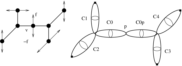
4.3. Degeneration formula
Given a FTCY graph with a bivalent vertex (see Figure 7), so that the relative FTCY 3-fold has a normal crossing singularity, we may either deform or resolve this singularity. Figure 8 shows the corresponding operation on the graph : is the smoothing of , and is the resolution of . The relative FTCY 3-folds
are smooth. The degeneration formula relates the relative formal Gromov-Witten invariants of the smoothing to those of the resolution .

Geometrically, given a relative stable map with
we degenerate and resolve to obtain a pair of maps to and to with degrees
and ramification patterns
(See Figure 8.) In this example, for , so we may suppress .
Conversely, given a pair of maps to and , with ramifications matching in the middle, we may glue and smooth to obtain a map to . The degeneration formula says exactly this:
where is some combinatorial factor. Here we consider which counts maps from possibly disconnected curves with instead of which counts maps from connected curves of genus , because the degeneration formula of is neater than that of .
4.4. Topological vertex
By degeneration and resolution, it remains to compute the formal invariants of the graph on the left hand side of Figure 9. The graph depends on three integers and two weights ; note that and the framings ’s are determined by ’s and ’s.

The invariants depend on the genus of the domain and three partitions , , corresponding to the ramification patterns along , , . Note that in this case the degrees is determined by ramification patterns .
Define
where , . A priori it depends on both the topological data and the equivariant data . In [30], the authors proved that it is indeed topological: it is a rational number depending on but not on .
can be viewed as local relative Gromov-Witten invariants of a configuration of three ’s embedded in a relative Calabi-Yau 3-fold such that the formal neighborhood is the relative FTCY 3-fold defined by the graph of a topological vertex. We expect the following two counting problems to be equivalent:
- (i)
Relative topological vertex. Counting multiple covers of a configuration of three spheres (Figure 9) embedded in a Calabi-Yau 3-fold relative to three divisors with ramification patterns .
- (ii)
Open topological vertex. Counting multiple covers of a configuration of three discs (Figure 1) embedded in a Calabi-Yau 3-fold relative to three Lagrangian submanifolds with winding numbers , , .
It is interesting to compare the above (i) and (ii) with the classical Hurwitz problem:
- (i)’
Counting ramified covers of the sphere by compact Riemann surfaces, with prescribed ramification pattern over .
- (ii)’
Counting ramified covers of the disk by bordered Riemann surfaces, with prescribed winding numbers .
The above two counting problems (i)’ and (ii)’ are equivalent; they both give rise to Hurwitz numbers.
We now introduce some notation. Given a partition , let be the length of the partition. Given a triple of partitions , let , and define a generating function
4.5. Localization
For later convenience, we consider a slightly modified generating function
This is a generating function of relative Gromov-Witten invariants in the winding basis. By localization calculations, these invariants can be expressed in terms of three-partition Hodge integrals and double Hurwitz numbers, which we define now.
The three-partition Hodge integrals are defined to be
where
Define a generating function
Let be the disconnected version of .
Let be disconnected double Hurwitz numbers which count possibly disconnected covers of with ramification patterns and over and . We define a generating function
Localization calculations yield the following expression:
| (12) |
4.6. Framing dependence
Let . Recall that for each partition of , there is an associated irreducible character of the symmetric group and an associated conjugacy class of . By Burnside formula,
| (13) |
Proposition 3 (framing dependence in the winding basis).
We introduce a generating function
These are relative Gromov-Witten invariants in the representation basis. The framing dependence in the representation basis is simple:
Proposition 4 (framing dependence in the representation basis).
Note that O3 in Section 3 implies
Up to now, we have defined invariants which have the same gluing formula and framing dependence as do.
4.7. Combinatorial expression
We have
Lemma 5.
| (14) | ||||
A formula of the two-partition Hodge integrals in terms of (the Chern-Simons invariants of the Hopf link) was derived in [35]. can be expressed in terms of the skew functions (see [44]):
This allows one to evaluate the relative Gromov-Witten invariants of the topological vertex in terms of . More precisely, let , and let be the Littlewood-Richardson coefficients. Then
- R3.
, where
4.8. Applications
We now have an explicit formula of all formal relative Gromov-Witten invariants of relative FTCY 3-folds (and in particular, Gromov-Witten invariants of all toric Calabi-Yau 3-folds) in terms of . This formula has computational and theoretical applications:
- A1.
It is significantly more efficient than the traditional algorithm described in Section 2. Given a toric Calabi-Yau 3-fold, the generating function of its Gromov-Witten invariants in all genera in a fixed degree is an infinite series. By this formula, this infinite series is equal to a finite sum in terms of symmetric functions.
- A2.
- A3.
One can use this formula to verify enumerative predictions by other string dualities, for example the geometric engineering (see [31]).
4.9. Comparison
The physical theory of the topological vertex predicts the following formula for :
- O3.
, where
5. GW/DT Correspondence and the Topological Vertex
Maulik, Nekrasov, Okounkov, and Pandharipande conjectured a correspondence between the GW (Gromov-Witten) and DT (Donaldson-Thomas) theories for any non-singular projective 3-fold [37, 38]. This correspondence can also be formulated for certain noncompact 3-folds in the presence of a torus action; the correspondence for toric Calabi-Yau 3-folds is equivalent to the algorithm of the topological vertex [37, 44]. For non-Calabi-Yau toric 3-folds the building block is the equivariant vertex (see [37, 38, 45, 46]) which depends on equivariant parameters. The GW/DT correspondence for all toric 3-folds has been proved in a recent work by Maulik-Oblomkov-Okounkov-Pandharipande [39].
Acknowledgments
I am very grateful to Professor Shing-Tung Yau, who has educated me and has been offering me tremendous help and support over the years. As my thesis advisor, Professor Yau encouraged me to study the mathematical aspect of the large duality and provided me opportunities to learn its newest developments from leading experts. It is my great pleasure to dedicate this article to Professor Yau on the occasion of his 59th birthday.
I would like to thank my collaborators Jun Li, Kefeng Liu, and Jian Zhou for the fruitful and pleasant collaboration.
References
- [1] M.F. Atiyah, R. Bott, The moment map and equivariant cohomology, Topology 23 (1984), no. 1, 1–28.
- [2] M. Aganagic, A. Klemm, M. Mariño, C. Vafa, The topological vertex, Comm. Math. Phys. 254 (2005), no. 2, 425–478.
- [3] M. Aganagic, M. Mariño, C. Vafa, All loop topological string amplitudes from Chern-Simons theory, Comm. Math. Phys. 247 (2004), no. 2, 467–512.
- [4] K. Behrend, Gromov-Witten invariants in algebraic geometry, Invent. Math. 127 (1997), no. 3, 601–617.
- [5] K. Behrend, B. Fantechi, Intrinsic normal cone, Invent. Math. 128 (1997), no. 1, 45–88.
- [6] K. Behrend, Y. Manin, Stacks of stable maps and Gromov-Witten invariants, Duke Math. J. 85 (1996), no. 1, 1–60.
- [7] L. Chen, Y. Li, K. Liu, Localization, Hurwitz Numbers and the Witten Conjecture, arXiv:math/0609263.
- [8] D.-E. Diaconescu, B. Florea, Localization and gluing of topological amplitudes, Comm. Math. Phys. 257 (2005), no. 1, 119–149.
- [9] C. Faber, Algorithms for computing intersection numbers on moduli spaces of curves, with an application to the class of the locus of Jacobians, New trends in algebraic geometry (Warwick, 1996), 93–109, London Math. Soc. Lecture Note Ser., 264, Cambridge Univ. Press, Cambridge, 1999.
- [10] C. Faber, R. Pandharipande, Hodge integrals and Gromov-Witten theory, Invent. Math 139 (2000), no.1, 173–199.
- [11] K. Fukaya and K. Ono, Arnold conjecture and Gromov-Witten invariant, Topology 38 (1999), no. 5, 933–1048.
- [12] W. Fulton, R. Pandharipande, Notes on stable maps and quantum cohomology, Algebraic geometry—Santa Cruz 1995, 45–96, Proc. Sympos. Pure Math., 62, Part 2, Amer. Math. Soc., Providence, RI, 1997.
- [13] R. Gopakumar, C. Vafa, On the gauge theory/geometry correspondence, Adv. Theor. Math. Phys. 3 (1999), no. 5, 1415–1443.
- [14] R. Gopakumar, C. Vafa, M-Theory and Topological Strings–II, arXiv:hep-th/9812127.
- [15] T. Graber, R. Pandharipande, Localization of virtual classes, Invent. Math. 135 (1999), no. 2, 487–518.
- [16] H. Hofer, K. Wysocki, E. Zehnder, A General Fredholm Theory I: A Splicing-Based Differential Geometry, J. Eur. Math. Soc. (JEMS) 9 (2007), no. 4, 841–876.
- [17] H. Hofer, K. Wysocki, E. Zehnder, A General Fredholm Theory II: Implicit Function Theorems, arXiv:0705.1310.
- [18] H. Hofer, K. Wysocki, E. Zehnder, Integration Theory for Zero Sets of Polyfold Fredholm Sections, arXiv:0711.0781.
- [19] A. Iqbal, All genus topological amplitudes and 5-brane webs as Feynman diagrams, arXiv:hep-th/0207114.
- [20] E.-N. Ionel, T. Parker, Relative Gromov-Witten invariants, Ann. of Math. (2) 157 (2003), no. 1, 45–96.
- [21] E.-N. Ionel, T. Parker, The symplectic sum formula for Gromov-Witten invariants, Ann. of Math. (2) 159 (2004), no. 3, 935–1025.
- [22] S. Katz, C.-C.M. Liu, Enumerative geometry of stable maps with Lagrangian boundary conditions and multiple covers of the disc, Adv. Theor. Math. Phys. 5 (2001), no. 1, 1–49.
- [23] M.E. Kazarian, S.K. Lando, An algebro-geometric proof of Witten’s conjecture, J. Amer. Math. Soc. 20 (2007), no. 4, 1079–1089.
- [24] Y.-S. Kim, K. Liu, A simple proof of Witten conjecture through localization, arXiv:math/0508384.
- [25] M. Kontsevich, Intersection theory on the moduli space of curves and the matrix Airy function, Comm. Math. Phys. 147 (1992), no. 1, 1–23.
- [26] M. Kontsevich, Enumeration of rational curves via torus actions, The moduli space of curves (Texel Island, 1994), 335–368, Progr. Math., 129, Birkhäuser Boston, Boston, MA, 1995.
- [27] A. Li, Y. Ruan, Symplectic surgery and Gromov-Witten invariants of Calabi-Yau 3-folds, Invent. Math. 145 (2001), no. 1, 151–218.
- [28] J. Li, Stable Morphisms to singular schemes and relative stable morphisms, J. Diff. Geom. 57 (2001), 509–578.
- [29] J. Li, A degeneration formula of Gromov-Witten invariants, J. Diff. Geom. 60 (2002), 199–293.
- [30] J. Li, C.-C.M. Liu, K. Liu, J. Zhou, A mathematical theory of the topological vertex, Geom. Topol. 13 (2009), 527–621.
- [31] J. Li, K. Liu, J. Zhou, Topological string partition functions as equivariant indices, Asian J. Math. 10 (2006), no. 1, 81–114.
- [32] J. Li, G. Tian, Virtual moduli cycles and Gromov-Witten invariants of algebraic varieties, J. Amer. Math. Soc. 11 (1998), no. 1, 119–174.
- [33] J. Li, G. Tian, Virtual moduli cycles and Gromov-Witten invariants of general symplectic manifolds, Topics in symplectic -manifolds (Irvine, CA, 1996), 47–83, First Int. Press Lect. Ser., I, Int. Press, Cambridge, MA, 1998.
- [34] C.-C.M. Liu, K. Liu, J. Zhou, A proof of a conjecture of Mariño-Vafa on Hodge Integrals, J. Differential Geom. 65 (2003), no. 2, 289–340.
- [35] C.-C.M. Liu, K. Liu, J. Zhou, A formula of two-partition Hodge integrals, J. Amer. Math. Soc. 20 (2007), no. 1, 149–184.
- [36] M. Mariño, C. Vafa, Framed knots at large , Orbifolds in mathematics and physics (Madison, WI, 2001), 185–204, Contemp. Math., 310, Amer. Math. Soc., Providence, RI, 2002.
- [37] D. Maulik, N. Nekrasov, A. Okounkov, R. Pandharipande, Gromov-Witten theory and Donaldson-Thomas theory I, Compos. Math. 142 (2006), no. 5, 1263–1285.
- [38] D. Maulik, N. Nekrasov, A. Okounkov, R. Pandharipande, Gromov-Witten theory and Donaldson-Thomas theory II, Compos. Math. 142 (2006), no. 5, 1286–1304.
- [39] D. Maulik, A. Oblomkov, A. Okounkv, R. Pandharipande, Gromov-Witten/Donaldson-Thomas correspondence for toric 3-folds, arXiv:0809.3976.
- [40] M. Mirzakhani, Weil-Petersson volumes and intersection theory on the moduli space of curves, J. Amer. Math. Soc. 20 (2007), no. 1, 1–23.
- [41] M. Mumford, Towards an enumerative geometry of the moduli space of curves, Arithmetic and geometry, Vol. II, 271–328, Progr. Math., 36, Birkhäuser Boston, Boston, MA, 1983.
- [42] A. Okounkov, R. Pandharipande, Gromov-Witten theory, Hurwitz numbers, and Matrix models, Algebraic geometry—Seattle 2005, 325–414, Proc. Sympos. Pure Math., 80, Part 1, Amer. Math. Soc., Providence, RI, 2009.
- [43] A. Okounkov, R. Pandharipande, Hodge integrals and invariants of the unknot, Geom. Topol. 8 (2004), 675–699.
- [44] A. Okounkov, N. Reshetikhin, C. Vafa, Quantum Calabi-Yau and classical crystals, The unity of mathematics, 597–618, Progr. Math., 244, Birkhäuser Boston, Boston MA, 2006.
- [45] R. Pandharipande, R.P. Thomas, Curve counting via stable pairs in the derived category, arXiv:0707.2348.
- [46] R. Pandharipande, R.P. Thomas, The 3-fold vertex via stable pairs, Geom. Topol. 13 (2009), 1835–1876.
- [47] P. Peng, A simple proof of Gopakumar-Vafa conjecture for local toric Calabi-Yau manifolds, Comm. Math. Phys. 276 (2007), no. 2, 551–569.
- [48] Y. Ruan, Topological sigma model and Donaldson-type invariants in Gromov theory, Duke Math. J. 83 (1996), no. 2, 461–500.
- [49] Y. Ruan, Virtual neighborhoods and pseudo-holomorphic curves, Proceedings of 6th Gökova Geometry-Topology Conference, Turkish J. Math. 23 (1999), no. 1, 161–231.
- [50] Y. Ruan, G. Tian, A mathematical theory of quantum cohomology, J. Differential Geom. 42 (1995), no. 2, 259–367.
- [51] Y. Ruan, G. Tian, Higher genus symplectic invariants and sigma models coupled with gravity, Invent. Math. 130 (1997), no. 3, 455–516.
- [52] B. Siebert, Gromov-Witten invariants of general symplectic manifolds, arXiv:dg-ga/9608005.
- [53] E. Witten, Two-dimensional gravity and intersection theory on moduli space, Surveys in differential geometry (Cambridge, MA, 1990), 243–310, Lehigh Univ., Bethlehem, PA, 1991.
- [54] J. Zhou, A conjecture on Hodge integrals, arXiv:math.AG/0310282.
- [55] J. Zhou, Localizations on moduli spaces and free field realizations of Feymann rules, arXiv:math.AG/0310283.