Fast and Quality-Guaranteed Data Streaming in Resource-Constrained Sensor Networks
ABSTRACT
In many emerging applications, data streams are monitored in a network environment. Due to limited communication bandwidth and other resource constraints, a critical and practical demand is to online compress data streams continuously with quality guarantee. Although many data compression and digital signal processing methods have been developed to reduce data volume, their super-linear time and more-than-constant space complexity prevents them from being applied directly on data streams, particularly over resource-constrained sensor networks. In this paper, we tackle the problem of online quality guaranteed compression of data streams using fast linear approximation (i.e., using line segments to approximate a time series). Technically, we address two versions of the problem which explore quality guarantees in different forms. We develop online algorithms with linear time complexity and constant cost in space. Our algorithms are optimal in the sense they generate the minimum number of segments that approximate a time series with the required quality guarantee. To meet the resource constraints in sensor networks, we also develop a fast algorithm which creates connecting segments with very simple computation. The low cost nature of our methods leads to a unique edge on the applications of massive and fast streaming environment, low bandwidth networks, and heavily constrained nodes in computational power. We implement and evaluate our methods in the application of an acoustic wireless sensor network.
Categories and Subject Descriptors
C.3 [Computer Systems Organization]: Special-Purpose and Application-Based Systems; G.1.2 [Mathematics of Computing-Numerical Analysis]: Approximation-Linear approximation
General Terms
Algorithms, Design, Performance
Keywords
Wireless Sensor Networks, Data Streaming, Linear Approximation
1 Introduction
In many emerging applications, massive data streams are monitored in a network environment. For example, large sensor networks are extensively used in wildlife monitoring, road traffic monitoring, and environment surveillance. Each sensor generates a data stream where new data entries (i.e., new readings) keep arriving in a continuous manner. In order to aggregate and analyze the massive streaming data under monitoring, it is often required to transmit the data streams in the network. Due to often limited communication bandwidth and other resource constraints, online compressing data streams continuously with quality guarantee rises as a natural, critical and practical demand in those applications.
Example 1 (Motivation)
We, the authors of this paper, are building an acoustic monitoring system using wireless sensor networks. Sensor nodes are deployed in a target area, while each node contains an acoustic sensor which samples sound signals continuously. The sensor nodes are connected by a wireless network.
The acoustic monitoring system has many applications. An appealing scenario is towards “smart conference hall.” By analyzing the data collected from an acoustic monitoring system deployed in a large conference place, we can identify and locate speakers as well as some of their activities. The information can be used to adjust the equipment such as the light system, the microphone system, the video monitoring system, and the air conditioning system. Another potential application is bird surveillance in wildness. By analyzing the bird sound collected using such a sensor network, ornithologists can study the distribution of birds and their behavior patterns.
Wireless sensor nodes which integrate sensors, processors, memory and wireless transceivers often are small and have only very limited computational power and communication bandwidth. For instance, the Chipcon radio chip in the broadly-used MICA2 motes [15] has the maximum transmission power of mA and the maximum bandwidth of kbps.
In our acoustic monitoring system, we use MICA2 motes. One technical challenge is that, although a sensor can sample the acoustic signals frequently, the acoustic data stream cannot be sent out in time due to the low bandwidth radio channel. Specifically, in order to make the data analysis useful, we need to sample human voice with the normal sampling rate of kHZ and 16 bits per sample. This sampling mode requires the bandwidth of kbps for 1 channel (mono) voice, which greatly exceeds the maximum bandwidth of kbps that an MICA2 mote can support.In addition, we cannot temporarily store a large number of samples since the memory size of MICA2 motes is only kb. The only technical solution to the bottleneck is to online compress data streams continuously and send out the compressed streams instead of the original streams through the network. Sending compressed streams can also reduce the power consumption of sensors on communication, and thus extend lifetime of sensors. In large environmental surveillance sensor networks, recharging or replacing batteries of sensor nodes is often very difficult or even impossible after the sensors are deployed.
Many data compression and digital signal processing methods have been developed to reduce data volume, such as Fourier transform [17], discrete cosine transform [14], Wavelets [2], linear predictive coding (LPC) [1], etc. However, those methods cannot be applied to data stream compression in sensor networks due to the high cost of those methods in time and space. Moreover, sensor nodes like MICA2 motes only have very limited computational power. For example, only simple arithmetic operations are supported by TinyOS [3], the operating system for MICA2 motes. Although it is possible to implement a mathematical module to calculate essential functions like sinusoid and exponential functions or use dedicated DSP chips for audio processing and compression, such complex modules are highly undesirable due to the limited memory size and computational capacity of MICA2 motes as well as the extra energy cost of dedicated DSP chips.
In this paper, we tackle the problem of online compression of data streams in the application context of sensor networks. Particularly, we aim at the fast linear approximation methods (i.e., using line segments to approximate a time series) with quality guarantee. We make the following contributions.
First, we model the piecewise linear approximation problem properly for data streams. Different from the conventional situations where the whole time series to be compressed and the required compression rate can be specified, a data stream is potentially unlimited, and the distribution is often unpredictable. We propose the error-bounded piecewise linear approximation problem to tackle those challenges. Second, we present fast online solutions with linear time complexity and constant cost in space. Our algorithms are optimal in the number of segments used to approximate a (potentially unlimited) time series. In other words, our algorithms create the minimum number of line segments even without knowing the future incoming data. To the best of our knowledge, we are the first to successfully devise algorithms with such strong guarantees. Third, to address the computational challenges in sensor nodes, we develop another online approximation algorithm that is particularly tailored for tiny sensor devices by requiring only very simple computation. The low cost nature of our methods leads to a unique edge on the applications of massive and fast streaming environment, low bandwidth networks, and heavily constrained nodes in computational power (e.g., tiny sensor nodes). Last, we implement and evaluate our methods in the application of an acoustic wireless sensor network. Our empirical evaluation clearly shows that our methods are highly feasible for resource-constrained wireless sensor networks.
The rest of the paper is organized as follows. In Section 2, we formulate and analyze the problem, and review the related work. Two online algorithms are developed in Section 3, and their optimality is studied in Section 4. In Section 5, we design an online approximation algorithm which is more economic in computation for tiny sensors. We report our implementation and evaluation of the proposed methods in an acoustic wireless sensor network in Section 6. The paper is concluded in Section 7.
2 Problem Definition and Related Work
In this section, we propose the error-bounded piecewise linear approximation problem for data streams. We also review the related work.
2.1 Problem Formulation
Piecewise linear approximation (PLA) is an effective method to compress a time series. A numeric data stream can be treated as a potentially unlimited time series. Thus, it is natural to explore whether we can compress a numeric data stream using the piecewise linear approximation method.

Let be a time series of points, and be the value of the -th point of . A (line) segment is a tuple where and and are two endpoints. is called the range of .
Given a time series , PLA uses a set of line segments as the approximation of the time series. Figure 1 elaborates the general idea, where three line segments, , , and , are used to approximate a time series. A line segment approximates the -th point of the time series by value
The compression comes from that the number of line segments used for approximation can be much smaller than the number of points in the time series. In the figure, the time series has points. three segments are used to approximate the time series, and each segments has endpoints. Thus, the 3 line segments only need points to represent. A compression ratio of is achieved. Generally, the endpoints in the segments are not necessarily positioned at some points in the time series (e.g., , , and in the figure).
Formally, a set of segments is a piecewise linear approximation of if (1) are segments; and (2) for each index , is either in the range of exactly one segment in , or there exist two segments such that and share the same endpoint at index . Clearly, using the segments, for every index , can give a value to approximate .
PLA for static time series has been well studied (e.g., [5, 6, 8, 12]). Most of the previous studies address an optimization problem as follows.
Problem 1 (Conventional PLA problem)
Given a time series of points and a number , find a set of segments as a piecewise linear approximation of such that the approximation error is minimized.
Unfortunately, solutions to the conventional PLA problem are not applicable to data streams. A data stream is potentially unlimited. It is impossible to know in advance the number of points in the stream or to specify the number of segments to be used for approximation. To tackle the stream compression problem, in this paper, we turn to the error-bounded PLA problem.
Problem 2 (Error-bounded PLA problem)
Given an error measurement function such that gives the error that a PLA approximates . Let be a user-specified error bound. is called an -PLA of if . An -PLA of is optimal if (i.e., the number of segments in ) is minimized.
We propose two error measurement functions meaningful for data streams.
First, the max-err function captures the maximal error between and at any index. That is,
With potentially unlimited streams, using the max-err function, we can make sure the approximation quality is consistently bounded at every point.
Second, the seg-err function checks the error introduced by each segment, and captures the maximal error. That is,
Using the seg-err function, we can make sure that the error introduced by every segment is bounded.
Using the two error measurement functions, we have two versions of the error-bounded PLA problem.
Problem 3 (PLA-PointBound problem)
Given an error-bound , the PLA-PointBound problem is to find an -PLA such that and is minimized.
Problem 4 (PLA-SegmentBound problem)
Given an error-bound , the PLA-SegmentBound problem is to find an -PLA such that and is minimized.
2.2 Related Work
Piecewise linear approximation (PLA) has been well investigated in [4, 7, 8, 12, 13, 16]. The idea behind PLA comes from the fact that a sequence of line segments can be used to represent the time series while preserving a low approximation error. Standard linear regression technique is widely used in most existing piecewise linear approximation algorithms to calculate a line segment approximating the original data with the minimum mean squared error. Many of them [5, 6, 8, 12] target at solving the conventional PLA problem and may not be applicable to streaming data.
Despite the substantial research efforts in PLA techniques [5, 6, 7, 11, 8, 12], existing solutions are not tailored for data streams over resource-constrained sensor networks. They either require complex computation or have high cost in space. To the best of our knowledge, there has no implementation of these algorithms in realistic sensor device.
In [9], the authors use PLA to estimate a time series. But the authors put unnecessary constraints on the algorithm, which requires the endpoints come from the original dataset. On the whole, their algorithm can run in time complexity and takes space complexity.
In [7], Keogh et al. give a comprehensive review on the existing techniques for segmenting time series. They categorize the solutions into three different groups, namely sliding window methods, top-down methods, and bottom-up methods. They then take advantage of both sliding window and bottom-up methods and design a Sliding-Window-And-Bottom-up (SWAB) algorithm. The SWAB algorithm uses a moving window to constrain a time period in consideration.
In [11], an amnesic function is introduced to give weights to different points in the time series. The PLA-SegmentBound problem is discussed in the context of Unrestricted Window with Absolute Amnesic (UAA) problem, but complete solutions to this problem are not provided in [11].
A solution to the PLA-PointBound problem is addressed in [10] with a different definition of point error bound. The algorithm is claimed to be optimal, but the time complexity is where is the number of points in the time series. Moreover, no performance evaluation of the solution is presented in the paper.
In summary, although the error-bounded PLA problem has been investigated before, the problem has not been studied systematically. No solutions applicable to data streams have been developed, let alone solutions for resource-constrained sensor networks.
3 Online Algorithms
In this section, we develop two online algorithms for the
PLA-PointBound and the PLA-SegmentBound problems, respectively. The
two algorithms share the same framework.
3.1 The Framework
The framework of our algorithms works in a greedy manner. When , the first point in the stream, arrives, we store . When arrives, we also store since and can be compressed by a segment exactly. When arrives, we check whether can be compressed together with and by a line segment satisfying the error-bound requirement. If so, we store . Otherwise, we output a line segment compressing and , remove and from the main memory, and store .
Generally, imagine we have a buffer in main memory storing points such that the points in the buffer can be compressed by a line segment satisfying the error-bound requirement. When a new point arrives, we check whether can be compressed together with by a line segment satisfying the error-bound requirement. If so, we add to the buffer and move on to the next point. Otherwise, we output a segment compressing satisfying the error-bound requirement, and remove them from the buffer. is then stored in the buffer.
Although the framework is simple, there are two critical issues that need to be solved carefully in order to make sure that the runtime of the algorithms is linear with respect to the number of points in the streams, and the space size needed by the algorithms is bounded by a constant.
First, how can we store the information about the points we have seen but have not compressed? In the worst case, there can be an unlimited number of such points (e.g., a times series where all points take the same value). How can we summarize them using only constant size memory?
Second, how can we determine whether a newly arrived point can be compressed together with the points already in the buffer that have been seen but have not been compressed? Revisiting those points one by one leads to the runtime quadratic with respect to the number of such points. As explained before, there can be an unlimited number of such points. The overall time complexity is quadratic if those points are revisited one by one.
Our central idea to tackle the above two challenges is the following. Instead of storing the points explicitly, we monitor the range of all possible line segments that can be used to compress the points that have been seen but have not been compressed in a concise way. When a new point arrives, we can check whether the point can be compressed using some line segment in the range. If so, it means that the new point can be compressed together with the points accumulated. We only need to adjust the range of the possible line segments to make sure the new point is also compressed. If not, it means that the new point cannot be compressed together with the points accumulated. A segment should be output.
3.2 Solving the PLA-PointBound Problem
A segment can also be represented by the left endpoint , the slope , and the index of the right endpoint .
For two points and in a data stream, if a line segment with slope can approximate and , i.e., and where is the error-bound, must satisfy the following four conditions.
| (1) |
| (2) |
| (3) |
| (4) |
Figure 2 illustrates the conditions and their relations. Particularly, and are the slopes of the two lines shown in the figure.

Since the line segments are determined by the value of the left endpoint and slope , we examine the distribution of points that satisfy Equations 1 to 4. As illustrated in Figure 3, the possible line segments form a polygon . We have the following important result.

Lemma 1 (PLA-PointBound)
A line segment of left endpoint and slope can approximate points with max-err at most if and only if is in polygon .
Proof. The necessity follows with the definition of . For any line segment , there exists an index such that , i.e., cannot approximate either or .
We prove the sufficiency by contradiction. Suppose a segment but cannot approximate . Two situations may arise. First, . Then, since where is the value of on index . Second, . Then, . In both cases, we have contradictions.
| Input: a data stream and error-bound ; | ||||
| Output: a list of line segments approximating | ||||
| such that ; | ||||
| Method: | ||||
| 1: | ; ; ; | |||
| 2: | WHILE (1) DO | |||
| 3: | ; | |||
| 4: | IF THEN , ; | |||
| 5: | ELSE | |||
| 6: | randomly choose a point in ; | |||
| /*any point in meets the point error bound*/ | ||||
| 7: | output a line segment | |||
| ; | ||||
| 8: | ; ; ; | |||
Using Lemma 1, we have algorithm PointBound, an online algorithm as shown in Figure 4. We maintain the intersection of polygons , …, , where is the first point that has not been compressed yet in the data stream, and is the last point arrived such that .
When a new point arrives, we compute and . If it is , then a line segment is randomly chosen to approximate such that is in , where is the value of on index , and is the slope of . is output, and the intersection of polygon is removed. and are used to generate a new polygon .
If , then the intersection is kept, and the algorithm moves on to the next point in the stream.
For any and , is a parallelogram where there are two edges parallel to the slope axis. It is easy to show that for any and , is a convex polygon. In the worst case, the edges of the intersection of parallelograms could be up to , i.e., twice the number of parallelograms intersected. A straightforward method keeping all edges of the intersection area still has the quadratic time complexity and linear space complexity, which are not applicable to data streams.
Fortunately, we do not need to record all edges of the intersection polygon. Instead, we need to record only up to edges to determine whether a new point can be compressed together with the points seen but not compressed.
Using Equations 1 to 4, it is easy to see that each parallelogram has two properties: (1) Each parallelogram has two vertical edges and two sloping edges with a negative slope value, as shown in Figure 3. The range of is the same for all parallelograms (i.e., ). (2) For , the absolute slope value of the two sloping edges in is strictly smaller than the absolute slope value of the two sloping edges in .
Let us focus on the intersection points of the upper sloping edge of parallelograms. The case for the lower sloping edges can be analyzed similarly.
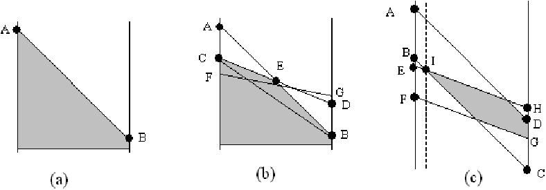
The situations are illustrated in Figure 5. Suppose that the first parallelogram gives the upper sloping edge with slope value as in Figure 5(a). When a new data point arrives, a new parallelogram is formed. In the worst case, the upper sloping edge of the parallelogram cuts into two parts. Let be the intersection point between and , as shown in Figure 5(b).
By the second property, we have . Moreover, the upper sloping edge of any future parallelogram cannot cut both and due to the smaller absolute slope value of than . In other words, if a future parallelogram intersects with the current intersection polygon, the upper sloping edge of the parallelogram can only cut either , or the right vertical edge. Instead of keeping and , we can keep line segment . Then, a future parallelogram intersects with the current intersection polygon if and only if it cuts .
Generally, we only need to keep the line segment connecting the left-most upper corner and the right-most upper corner for the upper sloping edges. Similarly, we only need to keep the line segment connecting the left-most lower corner and the right-most lower corner for the lower sloping edges.
In addition to this two line segments, we need to keep the two vertical edges in the intersection polygon. The reason is that the intersection of two parallelograms may shrink the range of the intersection, as illustrated in Figure 5(c), where parallelogram intersects with parallelogram . The left vertical edge is shrunk into a point right to the original edge.
In summary, we need to record only up to edges to determine whether a new point can be compressed together with the points seen but not compressed. This immediately leads to the following result.
Theorem 1 (Complexity – PointBound)
The algorithm PointBound for the PLA-PointBound problem has the time complexity and the space complexity , where is the number of points in a time series to be compressed.
Since algorithm PointBound only looks ahead for one point in the data stream to output a line segment whenever necessary in the piecewise linear approximation, it is an online algorithm and can be applied on data streams.
3.3 Solving the PLA-SegmentBound Problem
We first present the following useful observation, to which a similar result has been reported in [12] without proof.
Lemma 2
Suppose that a line segment approximates a fragment of points in a time series. Then, minimizes if the slope of is
| (5) |
and the left endpoint of has value
Proof. Consider a line segment approximating fragment . Let the left endpoint of be and the slope be . For each point , the error is . Thus,
| (6) |
Clearly, when , reaches the minimum value
| (7) |
From Equation (7), when
is minimized.
| Input: a data stream and error-bound ; | |||
| Output: a list of line segments approximating | |||
| such that ; | |||
| Method: | |||
| 1: | ; | ||
| 2: | the line segment ; | ||
| 3: | WHILE (1) DO | ||
| 4: | the line segment identified in Lemma 2 to | ||
| compress ; | |||
| 5: | IF THEN | ||
| 6: | ; ; | ||
| 7: | ELSE | ||
| 8: | output ; | ||
| 9: | ; ; | ||
| 10: | the line segment ; | ||
Lemma 2 leads to algorithm SegmentBound, an online algorithm for the PLA-SegmentBound problem as shown in Figure 6. Suppose are the points that have not been compressed yet. When a new point arrives, we check whether the line segment identified by Lemma 2 can achieve the segment error bound. If so, then is added into the buffer, and the algorithm moves on to the next point in the stream. Otherwise, the line segment suggested by Lemma 2 for points is output, and are considered compressed. is added into the buffer.
When a new data point arrives, the left endpoint and the slope of the line segment suggested by Lemma 2 can be calculated quickly. Technically, Equations (5) and (7) indicate that we need to calculate , , , , and . Since we already have ,, ,, and , the addition of the new point only incurs a constant cost to update the values of and the left endpoint. This leads to the following result.
Theorem 2 (Complexity – SegmentBound)
The algorithm SegmentBound for the PLA-SegmentBound problem has the time complexity and space complexity , where is the number of points in a time series to be compressed.
4 Optimality
Theorem 3 (PLA-PointBound quality)
The PointBound algorithm in Section 3.2 produces a minimum number of segments to compress a time series.
Proof. For a time series , let , where is an -PLA approximating (i.e., ). We conduct an induction on to show that algorithm PointBound outputs an -PLA of line segments.
(Base case) Consider , i.e., there exists a line segment that approximates the whole time series. According to Lemma 1, . Thus, algorithm PointBound finds a line segment approximating and .
(Induction) Assume that, when , algorithm PointBound finds an -PLA of line segments to approximate . Now, let us consider the case of , i.e., there exists an optimal -PLA that approximates .
Suppose that approximates . Let us assume that output by algorithm PointBound approximates points . Due to Lemma 1, . Thus, must approximate with the quality guarantee, i.e., . In other words, .
If , then points in can be approximated by an -PLA of line segments. According to the assumption, algorithm PointBound finds an -PLA of line segments approximating .
Suppose that . Since can be approximated by an -PLA of line segments, a proper subset must also be approximated by an -PLA of at most line segments. We only need to drop the segments approximating . According to the assumption, algorithm PointBound finds an -PLA of the minimum number of line segments to approximate points .
In summary, algorithm PointBound finds an -PLA of line segments approximating .
Similarly, we can also show the optimality of the SegmentBound algorithm.
Theorem 4 (PLA-SegmentBound quality)
The SegmentBound algorithm in Section 3.3 produces a minimum number of segments to compress a time series.
Although the number of line segments used to approximate a time series is a good measure on the compression quality, it is not directly translated to compression ratio. For example, in our methods, the endpoints of segments are not constrained. Thus, two points are needed to represent a segment. On the other hand, a PLA using connecting segments (i.e., two consecutive segments share the same endpoint) may use more segments but achieve a better compression ratio since only one point is needed to represent a segment except for the first segment.
Theorem 5 (Compression factor)
Algorithms PointBound and SegmentBound have an approximation factor of to the optimum compression factor that an -PLA can achieve.
Proof. We only show the case for the PointBound algorithm. The same argument applies to the SegmentBound algorithm.
For any time series of points, suppose that the PointBound algorithm approximates using line segments. Then, according to Theorem 3, any PLA cannot have less than line segments. To represent line segments, at least points are needed. Thus, the optimum compression ratio using PLA is at most .
The line segments generated by the PointBound algorithm may not be connecting. Thus, at most points are needed to represent the line segments. The worst case compression ratio of the PointBound algorithm is . Clearly, .
5 PLAZA for Tiny Sensors
Although algorithm PointBound is optimal for the PLA-PointBound problem, it still may be too computation intensive for tiny, resource-constrained sensors due to two reasons.
First, algorithm PointBound may generate non-connecting segments such that each segment requires the transmission of two endpoints. As analyzed before, connecting line segments reduce the data transmission volume since each segment (except the first one) requires the transmission of only one endpoint. Second, algorithm PointBound has to calculate intersection of parallelograms. The computation may be too heavy for tiny, resource-constrained sensor nodes.
In this section, we design a simple, fast online algorithm PLAZA (Piecewise Linear Approximation with Zoning Angle) for the PLA-PointBound problem. PLAZA generates connecting line segments. Although PLAZA is not optimal in the number of line segments used for approximation, it is light in computation and very effective in compression ratio, as will be verified by our experiments.
5.1 PLAZA
PLAZA builds on the concept of zoning angle. Given an error bound and two points and (), the zoning angle from to , denoted by , is defined as the angle that has as the endpoint, as the bisector, and has a degree of , where .
Figure 7(a) shows an example of zoning angle . The zoning angle defines a zone to include any potential line segments that can be used to compress and .
We observe the following important results. Their proof is trival and is omitted due to space limit.
Lemma 3
For three points in a time series, the line segment approximates with error up to if and only if the line segment falls in the zoning angle .
Lemma 4
For three points in a time series, if zoning angle has no overlap with zoning angle , there does not exist a line segment with as the left endpoint such that .
| Input: a data stream and error-bound ; | ||||
| Output: an -PLA of a list of connecting line | ||||
| segments, i.e., ; | ||||
| Method: | ||||
| 1: | ; ; | |||
| 2: | line segment ; ; | |||
| 3: | WHILE (1) DO | |||
| 4: | ; | |||
| 5: | IF THEN | |||
| 6: | IF segment falls in | |||
| 7: | THEN line segment ; | |||
| 8: | ELSE | |||
| 9: | = the value of the bisector line of | |||
| at index as shown in Figure 7(b); | ||||
| 10: | the line segment ; | |||
| 11: | ; | |||
| 12: | ||||
| 13: | ; | |||
| 14: | ||||
| 15: | ELSE | |||
| 16: | output ; | |||
| 17: | ; ; ; | |||
| 18: | ; | |||
| 19: | line segment ; | |||
| 20: | ||||
| 21: |
Algorithm PLAZA works as follows. Starting from a point , Lemma 3 is used to check if there is a line segment approximating points between indexes and . Moreover, Lemma 4 is used to check if searching further in the time series is futile. The pseudocode of PLAZA is shown in Figure 8. Algorithm PLAZA scans each point in a data stream only once and stores only the zoning angle and the current approximating segment in main memory, the algorithm clearly has linear time complexity and constant space complexity.
5.2 Benchmarking PLAZA
PLAZA creates connecting line segments. Only transmission of one point is needed for each line segment except for the first line segment. This feature distinguishes PLAZA from algorithms PointBound and SegmentBound. What is the optimal compression that can be achieved by an -PLA consisting of only connecting line segments?
The idea behind the optimal PLAZA benchmark algorithm is similar to that of algorithm PointBound. The main difference is that, unlike the PointBound algorithm, we do not start the new segment with the initial condition , where is the value of the left endpoint of the new segment. Instead we set a smaller range on to guarantee the connectivity of two consecutive segments. Specifically, to decide the range of , we use the last non-empty polygon intersection in the previous point.
We find the optimal solution by a thorough search. Starting from , we try all values of such that can be approximated by a line segment with maximal error . For each such a subset , we compute the intersection of parallelograms , and try to find a line segment with left endpoint that can approximate some points where and is in the range confined by . By doing so, the first and the second line segments are connected. We conduct a depth-first search to find an -PLA consisting of the minimum number of connecting line segments. Limited by space, we omit the details here.
The optimal PLAZA benchmark is an offline algorithm: it assumes the time series is given and can be scanned multiple times. Its complexity is far above linear due to the thorough search. This algorithm is obviously not suitable for online compression of data streams. It is for comparison purpose only.
6 Experimental Evaluation
In this section, we evaluate the performance of our online algorithms by simulation in Matlab and by real implementation with MICA2 motes [15].
6.1 Experimental Setting
We generated two audio files for test. The first file includes human voice with the sampling rate of khz in mono channel. The second file includes piano music with the sampling rate of khz in mono channel. Each file includes samples, and the size of each sample is bits. Figures 12 and 12 show the waveform of the human voice data and the waveform of the piano music, respectively. It can be seen that the music data is much “smoother" than the human voice data. We use the files to test the performance of our online algorithms in bandwidth saving. We measure two metrics:


- 1.
Sample reduction ratio (inverted compression ratio). It is defined as the total number of points to represent the -PLA divided by the total number of points in the original time series.
- 2.
Distortion. It is defined as , where is the total number of points in the time series, is the original value, and is the approximated value of .
In simulation, we apply the online algorithms on the audio files and measure the sample reduction ratio. Simulation results are reported in Section 6.2 and Section 6.3. In the test using MICA2 motes, the original audio files are played on a desktop computer and are monitored and transmitted with a MICA2 mote over wireless channel to a laptop computer. More details are provided in Section 6.4.
6.2 Results on Quality
6.2.1 Results on Sample Reduction Ratio
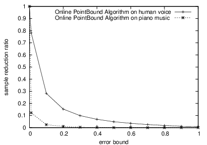
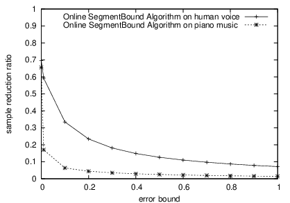
Figures 12 and 12 show the results of algorithms PointBound and SegmentBound, respectively, with respect to various error bound values. As shown in the figures, we can obtain a higher bandwidth saving on piano music than on human voice. By replaying the audio files recovered from the samples by our algorithms, we perceive that the human voice recovered from the samples by our algorithms is fully recognizable with the segment error bound up to , or with the point error bound up to . The quality of recovered piano music is acceptable to us with the segment error bound up to , or with the point error bound up to .
Figures 12 and 12 clearly demonstrate significant bandwidth saving. With the online algorithms, we only need to transmit around of the original sample size for piano music and around of the original sample size for human voice. As such, both sound files can be transmitted with the current sensor nodes.
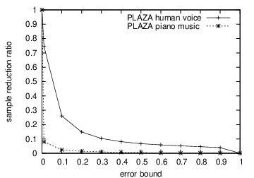
Figure 13 shows the sample reduction ratio of algorithm PLAZA with respect to various point error bounds. We can observe the similar phenomenon as in Figures 12 and 12. With PLAZA, we perceive that the recovered human voice is fully recognizable with the (point) error bound up to , and the quality of recovered piano music is acceptable to us with the (point) error bound up to . From Figure 13, the above qualities correspond to the bandwidth reduction of nearly of the original data size for piano music and about of the original data size for human voice.
One interesting phenomenon is that the SegmentBound algorithm can reduce sample transmission volume even if the error bound is set to zero, as shown in Figure 12. This is because in the audio files, there are some silent periods where the sample values are close to zeros. The SegmentBound algorithm finds a line segment to approximate those situations. This nice feature, however, does not exist in the algorithms for the PLA-PointBound problem. If the error bound is zero, the initial polygon is empty in the PointBound algorithm, and the degree of the initial feasible angle is zero in PLAZA, resulting in no sample reduction.

Figure 14 compares algorithms PLAZA, PointBound, and
SegmentBound on the human voice data set. The gap between algorithms
PLAZA and PointBound is very small when the error bound is less than
. Algorithm PointBound leads to more samples than algorithm
PLAZA when the error bound is less than . The gap between
algorithm SegmentBound and the two algorithms for the
PLA-PoinBound problem comes from the fact that, using the same error
bound value, the PLA-SegmentBound problem puts a tighter error
constraint than the PLA-PointBound problem. We observe the similar
performance comparison of the three algorithms on the piano data
set, but omit the figures here due to space limit.
6.2.2 Results on Distortion


In Figures 16 and 16, we quantitatively show the distortion of our algorithms on the human voice data set and the piano music data set, respectively. The overall distortion on human voice is larger than that on piano music due to the “smoother" waveform in the music data set. With the same error bound, algorithm PLAZA has the largest distortion. Algorithm PointBound is the next. Algorithm SegmentBound has the smallest distortion because the same error bound on the PLA-SegmentBound problem and the PLA-PointBound problem poses a tighter error constraint on the PLA-SegmentBound problem. The smaller distortion, however, comes with the cost of lower bandwidth saving as analyzed before.
6.3 Benchmarking PLAZA
We test the performance of PLAZA comparing to the optimal solution of its kind (i.e., using connecting line segments to tackle the PLA-PointBound problem). Due to the high complexity of the PLAZA Benchmark method, the audio files are too big to obtain the optimal results within reasonable time. We have to use a small portion of the audio files for this test.
Interestingly, the PLAZA method and the optimal PLAZA benchmark algorithm generate very similar PLA line segments. Audio files are usually filled with short silent periods where sample values are close to . Thus, algorithm PLAZA can obtain line segments very similar to those computed by the benchmark algorithm. We omit the detailed figures due to space limit.
6.4 Results on Real Sensors
We implemented our online algorithms using MICA2motes [15] from Crossbow Technology Inc. The test bed is illustrated in Figure 17. A MICA2 mote includes a radio/processor board and a sensor board. The radio/processor board uses Mhz radio. The sensor board includes a microphone that can be used for sampling sound. The interface of the base station is based on RS232. It acts as a gateway to connect the laptop and the radio wireless sensor network. The original audio files are played on a desktop computer, monitored by a MICA2 mote, and transmitted over wireless channel from the MICA2 mote to the base station.

The results about the sample reduction ratio on the real sensor test bed are close to the simulation results using Matlab. But the audio quality obtained using the real test bed is worse than that obtained in the Matlab simulation. The deterioration in audio quality is caused by the major restriction of TinyOS [3], the current operating system in MICA2 motes. The OS does not support multiple threads and thus it cannot perform radio transmission and sound sampling concurrently. Due to this limit, when we transmit data to the base station, the sensor board stops sampling and the sound during this period is missed, resulting in small silent gaps in the recovered audio. Nevertheless, we can still recognize the human speech and the piano music.
The same task can be carried out with the most recent, more advanced sensor device, MICAz from the same company. With a higher price, MICAz sensors support up to Kbps wireless transmission. This task, however, has never been fulfilled with low-end devices like MICA2. To this end, we break the limit of scarce radio bandwidth and carry out a task that is hard to achieve without our fast online compression methods.
6.5 Evaluation in Other Applications
Although we only implemented the online algorithms in an acoustic sensor monitoring system, our algorithms are actually applicable to many other application domains such as electrocardiogram (ECG) monitoring for patients. We test our algorithm on an ECG data set The maximum value on the data set is and the minimum value is . We test our online algorithms with error bound varying from to .

Figure 18 compares the sample reduction ratio of algorithms PLAZA, PointBound, and SegmentBound on the ECG data set. The performance of algorithms PLAZA and PointBound is very similar. When the error bound is set to over , both algorithms can compress the data up to of the original size. The gap between algorithms SegmentBound and PointBound comes from the fact that, using the same error bound, the PLA-SegmentBound problem and the PLA-PointBound problem put a tighter error constraint on the PLA-SegmentBound problem.
7 Conclusion
In this paper, we tackle the problem of online compression of data streams in the resource-constrained network environment, where the traditional data compression techniques cannot apply. Particularly, we aim at fast piecewise linear approximation (PLA) methods with quality guarantee. We study two versions of the problem which explore quality guarantees in different forms. For the error bounded PLA problem, we design fast online algorithms running in linear time complexity and requiring a constant space cost. The online algorithms are also optimal in terms of the number of generated segments. To meet the needs from tiny, resource-constrained sensors, we develop another online algorithm that involves very simple computation and generates connecting line segments. Our simulation results and the test using a real sensor test bed demonstrate that our fast online linear approximation methods are very effective for data stream compression and transmission over low bandwidth networks with nodes heavily constrained in computational power.
Equipped with the insights gained in this study, we see a lot of application opportunities for our methods. Meanwhile, there are also some interesting open questions for future work. For example, an interesting question is to design an online algorithm that can compute an -PLA consisting of connecting line segments that has an approximation factor to the optimum.
Acknowledgement
This research was supported by Natural Sciences and Engineering Research Council of Canada (NSERC), Canada Foundation for Innovation (CFI), and the British Columbia Knowledge Development Fund (BCKDF). We also thank Dr. E. Keogh for his informative comments and for providing the ECG dataset.
References
- [1] B. S. Atal and L. S. Hanauer. Speech analysis and synthesis by linear prediction of the speech wave. Journal of the Acoustical Society of America, 50:637–655, 1971.
- [2] K.P. Chan and A. W. Fu. Efficient time series matching by wavelets. In ICDE ’99: Proceedings of the 15th International Conference on Data Engineering, pages 126–133, Washington, DC, USA, 1999. IEEE Computer Society.
- [3] D.E. Cull, J. Hill, P. Bounadonna, R. Szewczyk, and A. Woo. A network-centric approach to embedded software for tiny devices. In Proceedings of First International Workshop on Embedded Software (EMSOFT 2001), Tahoe City, CA, October 2001.
- [4] D. H. Douglas and T. K. Peucker. Algorithms for the reduction of the number of points required to represent a digitized line or its caricature. Canadian Cartographer, 10(2):112–122, December 1973.
- [5] J. G. Dunham. Optimum uniform piecewise linear approximation of planar curves. IEEE Trans. Pattern Anal. Mach. Intell., 8(1):67–75, 1986.
- [6] M. T. Goodrich. Efficient piecewise-linear function approximation using the uniform metric: (preliminary version). In SCG ’94: Proceedings of the tenth annual symposium on Computational geometry, pages 322–331, New York, NY, USA, 1994. ACM Press.
- [7] E. Keogh, S. Chu, D. Hart, and M.J. Pazzani. An online algorithm for segmenting time series. In ICDM, pages 289–296, 2001.
- [8] E. Keogh and M. Pazzani. An enhanced representation of time series which allows fast and accurate classification, clustering and relevance feedback. In Fourth International Conference on Knowledge Discovery and Data Mining (KDD’98), pages 239–241, New York City, NY, 1998. ACM Press.
- [9] C. Liu, K. Wu, and J. Pei. An energy efficient data collection framework for wireless sensor networks by exploiting spatiotemporal correlation. IEEE Transactions on Parallel and Distributed Systems, 18:1010–1023, July 2007.
- [10] G. Manis, G. Papakonstantinou, and P. Tsanakas. Optimal piecewise linear approximation of digitized curves. In Digital Signal Processing Proceedings, 1997. DSP 97., 1997 13th International Conference, pages 1079–1081. IEEE Computer Society, 1997.
- [11] T. Palpanas, M. Vlachos; E. Keogh, D. Gunopulos, and W. Truppel. Online amnesic approximation of streaming time series. In Data Engineering, 2004. Proceedings. 20th International Conference, pages 339–349, 2004.
- [12] Y. Qu, C. Wang, and X.S. Wang. Supporting fast search in time series for movement patterns in multiples scales. In Proceedings of the 7th ACM CIKM Int’l Conference on Information and Knowledge Management, pages 251–258, November 1998.
- [13] H. Shatkay and S. Zdonik. Approximate queries and representations for large data sequences. In Proceedings of the 12th IEEE International Conference on Data Engineering, February 1996.
- [14] D. Sinha and J.D Johnston. Audio compression at low bit rates using a signal adaptive switched filterbank. In Acoustics, Speech, and Signal Processing, 1996. ICASSP-96. Conference Proceedings., 1996 IEEE International Conference, volume 2, pages 1053–1056. IEEE Computer Society, 1996.
- [15]
Crossbow Technology.
Mica2 mote datasheet.
"http://www.xbow.com/Products/
Product_pdf_files/Wireless_pdf/MICA2_Datasheet.pdf". - [16] C. Wang and S. Wang. Supporting content-based searches on time series via approximation. In Proceedings of the 12th International Conference on Scientific and Statistical Database Management, July 2000.
- [17] Y. Wu, D. Agrawal, and A. Abbadi. A comparison of dft and dwt based similarity search in time-series databases. In CIKM ’00: Proceedings of the ninth international conference on Information and knowledge management, pages 488–495, New York, NY, USA, 2000. ACM Press.