Interference of heavy holes in an Aharonov-Bohm ring
Abstract
We study the coherent transport of heavy holes through a one-dimensional ring in the presence of spin-orbit coupling. Spin-orbit interaction of holes, cubic in the in-plane components of momentum, gives rise to an angular momentum dependent spin texture of the eigenstates and influences transport. We analyze the dependence of the resulting differential conductance of the ring on hole polarization of the leads and the signature of the textures in the Aharonov-Bohm oscillations when the ring is in a perpendicular magnetic field. We find that the polarization-resolved conductance reveals whether the dominant spin-orbit coupling is of Dresselhaus or Rashba type, and that the cubic spin-orbit coupling can be distinguished from the conventional linear coupling by observing the four-peak structure in the Aharonov-Bohm oscillations.
pacs
03.65.Vf, 71.70.Ej, 73.23.-b, 73.63.-bI Introduction
Conductance of mesoscopic rings threaded by the magnetic flux shows Aharonov-Bohm oscillations [1] due to the phase a quantum state acquires when it winds around the magnetic flux. An analogous effect in rings made of semiconductors with spin-orbit coupling occurs due to the spin precession as an electron orbits the ring, giving rise to the Aharonov-Casher phase [2]. Both the Aharonov-Bohm and the Aharonov-Casher effect are manifestations of quantum coherence in mesoscopic systems, and provide a way to study the quantum interference in mesoscopic conductors [3, 4, 5, 6]. They lead to universal conductance fluctuations [7] and persistent spin and charge currents [9, 10, 8]. From a more practical point of view, the conductance that depends on the magnetic flux in the case of Aharonov-Bohm effect, or on the strength of spin-orbit coupling in the case of Aharonov-Casher effect, paves the way for novel applications in mesoscopic electronic and spintronic devices. For example, the Aharonov-Casher phase can be modified by applying a backgate voltage to the device and changing the Rashba coupling constant [11]. This enables spintronic devices that require neither any ferromagnetic materials, nor the control over magnetic field to operate [11, 12, 13, 14].
Recently, a number of experimental [16, 15] and theoretical [4] studies have investigated transport of heavy holes in rings. These studies are relevant because of the strong spin-orbit coupling of heavy holes confined to the ring [15], and long coherence length ( in carbon-doped GaAs), making the interference effects in transport observable. The material parameters of holes allow for spintronic applications [17]. In coherent spin-orbit coupled systems, the transport shows an intriguing interplay of Aharonov-Bohm and Aharonov-Casher effects [18]. Apart from showing strong spin-orbit coupling and long coherence lengths, the heavy holes interact through a novel form of the spin-orbit coupling that is cubic in the in-plane components of momentum. This form of spin-orbit coupling influences the interference effects in transport.
In this work, we study the conductance of a ring of heavy holes tunnel-coupled to two external leads. This is in contrast to previous studies which consider rings that are strongly coupled to the leads [4], or are in a diffusive regime and can be described using semiclassical trajectories [19], or described in a lattice model [20]. Studies of the conduction through quantum dots embedded in an Aharonov-Bohm ring have focused on the effects of interaction on the transport [21, 22, 23] , while we study the interference of many available paths. In these setups, the interference effects can be traced to the Aharonov-Bohm and Aharonov-Casher phases accumulated by a spin experiencing a time dependent field while moving along a trajectory through the ring. In the adiabatic limit, this approach leads to geometric phases [24]. On the other hand, in our tunneling setup, the quantum effects in transport arise from the interference of tunneling paths through the eigenstates of the ring. The interference is then related to the magnetic field dependence of the eigenstates of a hole confined to the ring, and not to the phase accumulated by a spin following quasiclassical trajectory.
The states of a heavy hole orbiting a ring can be described in terms of pseudospin textures. At a position along the ring, the heavy hole state is
| (1) |
and it determines a unique direction in the pseudospin space for which is an eigenstate of pseudospin projection to the axis , i.e., . We identify the heavy hole states with pseudospin- pointing in direction, . The pseudospin texture associates the direction with every point on the ring (Figs. 1, 2), so that the states in Eq. (1) can be represented in terms of spin texture as
| (2) |
with the texture defined by the position-dependent unit vector , and the position-dependent overall phase . The textures of heavy hole eigenstates depend on the hole orbital momentum , so that the holes arrive at the connecting leads with different pseudospins, causing an interference pattern in the resulting conductance.
In the measurement of conductance as a function of flux through a semiconductor ring, the Aharonov-Casher effect manifests itself through an additional structure in the Aharonov-Bohm oscillations due to spin precession in the arms of the ring [15]. In the approximation of spin-orbit coupling that is linear in momentum, the conductance oscillations reveal a splitting of Aharonov-Bohm peak in the Fourier transform of resistivity as a function of the external magnetic field [25]. However, the spin-orbit coupling of holes in III-V semiconductors is, in lowest order, cubic in the hole momentum [26]. In this case, the spin texture of the orbiting carrier depends on the momentum (see below) and profoundly influences the transport. Therefore, for the carriers with cubic spin-orbit coupling, the Aharonov-Casher phase can be controlled by changing the momentum of the carriers, without the need to modify the coupling constant. This point is especially important in the structures fabricated in symmetric quantum wells where the Rashba coupling is absent, and the Dresselhaus spin-orbit coupling is given by the crystalline structure. Even though the coupling constant is fixed, due to the cubic form of spin orbit coupling, the Aharonov-Casher phase can still be indirectly controlled through the manipulation of the carrier momentum. In addition, the Dresselhaus and Rashba terms produce different patterns in conductance as a function of backgate voltage, so that the conductance in phase-coherent rings reveals the dominant type of spin-orbit coupling.
The remainder of the paper is organized as follows: In Sec. II, we describe the confinement of heavy holes to a ring and derive the effective one-dimensional Hamiltonian. In Sec. III, we solve for the hole eigenstates and eigenenergies. In Sec. IV, we introduce the tunnelling model of hole transport through the ring. In Sec. V, we present the resulting differential conductance of the ring. We conclude in Sec. VI.
II Heavy holes in a one-dimensional ring
Heavy holes confined to the two-dimensional hole gas (2DHG) are described with , where is the standard kinetic term, is the Zeeman coupling to the magnetic field , being the Bohr magneton, the gyromagnetic tensor of the confined holes, and the vector of the pseudospin Pauli matrices. The spin-orbit interaction of heavy holes is, in lowest order, cubic in the in-plane components of the momentum [26],
| (3) |
where and are respectively interaction strengths of Rashba and Dresselhaus spin-orbit coupling, and , (). The pseudo-spin represents the two heavy hole states . This is in sharp contrast to the electrons in a two-dimensional electron gas (2DEG), where the spin-orbit is in the lowest order linear in momentum. Effects of spin orbit coupling in general depend on the confinement, both to the 2DHG and to the ring. We will treat the spin-orbit coupling strengths and as free parameters and absorb the influence of the electrostatic potential that confines the holes to two dimensions into their values. In particular, if the confinement to two dimensions is caused by a symmetric potential, the Rashba coupling vanishes, . We neglect the orbital effects of the magnetic fields so that is the kinetic momentum of the hole.
In order to illustrate the spin structure of ring eigenstates, we will first solve for the eigenvalues and wave functions of the heavy holes confined to the ring in the absence of magnetic field. Later, we take the magnetic field into account and find that it causes modification of the quantization condition and the Zeeman coupling.
The two-dimensional hole gas is confined to the ring by a radial potential that has a deep minimum in the interval , where is the radius of the ring, and is its width. States of the hole orbiting the ring in the limit of strong confinement are products of the ground state radial wave function in the potential , and a function of the angular coordinate . For strong radial confinement, the motion of the hole in the ring is described by an effective Hamiltonian that depends only on the angular coordinate along the ring and all the properties of the radial wave function enter the problem only through the parameters of the effective one-dimensional Hamiltonian. The description in terms of the effective one-dimensional Hamiltonian is valid when both the energy spacing of the 2DHG confinement and the energy spacing of the radial confinement are much larger than the energies associated with the motion along the ring.
We find an effective Hamiltonian for the ring by introducing the confinement potential in the radial direction in and reducing it to the subspace of the lowest radial mode, in analogy with [27]. Typically these results were obtained by introducing a model potential and explicitly calculating the angular Hamiltonian for the lowest radial mode. The resulting one-dimensional effective Hamiltonian for the harmonic radial confinement was found for the case of linear- [27] and cubic Rashba [19] spin-orbit coupling. We note that generically the solution to the radial problem in an arbitrary potential can lead to divergences in the effective Hamiltonian. This can be avoided by working directly with the radial wave function in the form of a harmonic oscillator ground state. In this work, we employ a different approach, and calculate the effective Hamiltonian for a general radial wave function. The resulting effective one-dimensional Hamiltonian is
| (4) |
where , , , and , , , , and . The parameters that depend on the radial confinement are , where the expectation value is taken in the ground state radial wave function. The parameters , , satisfy consistency conditions that reduce the number of free parameters to two. We keep the explicit dependence of the independent expectation values in the radial state. The constraints are and . The constraints can be proven using integration by parts in the radial part of the Schrödinger equation, under the assumption that the radial part of the wave function vanishes at the origin together with its derivatives up to order 3. We have checked that this conclusion holds in the limit of a series of potentials that converge to the hard wall. Also, note that the relation between and is satisfied for the radial wave functions of the harmonic confinement for which diverges [19]. We can take the values and as the free parameters of the ring confinement. For a ring of radius and width , , .
Before embarking on the solution of the one-dimensional problem, let us briefly discuss the resulting Hamiltonian. Depending on the radius and the width of the ring, different terms in the spin-orbit interaction become more or less important. Also, we see an enhancement of the spin-orbit effects in narrow and small rings. We see that the strength of the spin-orbit coupling terms depends on the width of the one-dimensional ring through the parameter . This means that the spin-orbit coupling terms can be enhanced in a very narrow ring. In this limit, however, the spin-orbit coupling is effectively linear. Therefore, the effects of the cubic spin-orbit coupling presented here will be pronounced in the rings of intermediate widths, and the strength of radial confinement that is strong enough for the approximation of the single radial mode to hold.
III Spectrum and eigenstates of the orbiting holes
The effective Hamiltonian (4) describes a ring of heavy holes in the presence of both Dresselhaus and Rashba spin-orbit interaction, when and . Our goal is to understand the role of cubic spin-orbit coupling in transport, and contrast its effects to the standard linear spin-orbit coupling, experienced by the electrons in a similar configuration. We will therefore focus on the two limits that allow for a simple solution, namely, Dresselhaus-only interaction (), and Rashba-only interaction () that was previously studied in [19]. While restricting the domain of validity of our results, these approximations emphasize the physical picture of the eigenstates in terms of holes orbiting the ring, and the associated texture of the hole pseudospin. Apart from allowing a simple solution and providing a simple picture of the eigenstates, these two limits are also, in principle, realizable in practice. In the semiconductor heterostructures that confine holes to the 2DHG, the strength of the Rashba term is governed by the asymmetry of the confining potential in the direction perpendicular to the 2DHG plane. For a highly asymmetric potential the Rashba term is dominant, but it vanishes when the holes are confined by a symmetric potential well.
III.1 Dresselhaus () case
Eigenstates of the effective Hamiltonian (4) are specified by two quantum numbers, , where is an integer, and the texture quantum number , that takes on two discrete values. The Dresselhaus interaction eigenstates are
where the texture angle is
| (9) |
The states represent a hole that orbits the ring with angular momentum and well defined spin texture. At the point on the ring with the angle , the spin state corresponds to the spin that is tilted by the angle from the normal to the plane of the ring, and the azimuthal angle is , so that the projection of the spin to the plane of the ring is always tangential to the ring (see Fig. 1). The spin state associated with the other texture, , corresponds to the spin with the tilt angle , and the same azimuthal angle. The crucial difference with respect to the eigenstates of the ring with linear spin-orbit coupling is that the texture of the state depends on the momentum quantum number even in the absence of magnetic fields. Therefore, the states of different momentum show different spin textures.
Energies depend on both momentum and the texture,
| (10) |
The pairs of eigenstates form Kramers doublets, .

III.2 Rashba () case
When the spin-orbit coupling is of the Rashba type, the momentum for integer is still a good quantum number, and there are still two textures, and for every value of . The eigenstates are
with the Rashba texture angle
| (15) |
As for the Dresselhaus case, the eigenstates represent a hole with well defined pseudospin texture that orbits the ring. The texture is however quite different. The pseudospin is tilted away from the normal to the ring plane by the angle that, in contrast to the Dresselhaus case, can vary in the full range , while the Dresselhaus spin orbit coupling allows only for , except for and unrealistically large . The pseudospin projection to the plane of the ring, that was always tangential in the Dresselhaus case, now makes three full rotations on each orbit (see Fig. 2). The pseudospin of the opposite texture has the tilt angle , and the same projection to the ring plane.
Energies in the Rashba case again depend on the momentum and texture
| (16) |
The time reversal symmetry imposes Kramers degeneracy, and the states in the Kramers doublet have the same energy .

III.3 Magnetic field
Our preceding calculation of the eigenstates and eigenenergies did not take into account the interaction of holes with the magnetic field . In this subsection, we will find the spectrum and the eigenstates of a heavy hole in the presence of a magnetic field normal to the ring. This calculation includes the change of the quantization condition for the orbital momentum and the Zeeman term , but neglects the modification of the lowest energy radial wave function due to the magnetic confinement. This approximation neglects the modification of the radial confinement, described by and in Eq. 4 due to magnetic field. This approximation is valid for weak magnetic fields that give the cyclotron radius much larger than the ring radius , as well as for the magnetic fields of arbitrary strength confined to the interior of the ring.
The requirement that the wave function of an orbiting hole is single-valued, gives the quantization condition , for integer . In the absence of Zeeman coupling, the complete spectrum of the ring is periodic in the flux with the period . This perfect periodicity of the spectrum is broken by the Zeeman interaction.
For the magnetic field in direction, normal to the plane of the ring, it is possible to account exactly for the effects of Zeeman term , where is the magnetic field in with absorbed Bohr magneton and the gyromagnetic tensor component . For 2DHG the -tensor is highly anisotropic, and to a good approximation the only nonzero component is . Therefore, this approximation is valid also for the magnetic fields with in-plane components, with the adjustment that , since only the component impacts both the Aharonov-Bohm flux and the Zeeman term.
The Zeeman interaction couples the states of the same orbital momentum and opposite textures. The energies and eigenstates in the presence of Zeeman interaction are and , where
| (17) |
The eigenstates in the presence of Zeeman interaction keep the quantum numbers, but the states of opposite textures get mixed
| (18) |
where the mixing angle is
| (19) |
Here is the energy difference of the two states with momentum and opposite textures.
IV Tunneling model of conduction
We consider a system of heavy holes confined to a ring-shaped geometry and contacted by a pair of leads [Fig. 3].

The lead density of states is assumed to be wide and flat. In order to elucidate the pseudospin structure of the leads, we allow for an arbitrary pseudospin density matrix in the source(drain) lead.
The spin textures revealed in the eigenstates of heavy holes confined to a ring influence the transport properties when the ring is coupled to electrodes. For example, the hole of a given pseudospin entering the ring from the source electrode can propagate via different eigenstates, and arrive at the drain electrode with different pseudospin orientations. The pseudospin states at the drain electrode will interfere, and the probability of transmission will depend on the pseudospin orientations. Since the pseudospin orientations at the drain electrode depend on the hole momentum through the texture of the state , we may expect that the transmission of the ring, and therefore the resulting conductance will also depend on the momentum of the incoming hole. This momentum dependence is absent the electronic systems where the texture is determined solely by the spin-orbit coupling constant [28]. Therefore, we expect new effects of spin interference in transport of carriers that are subject to the cubic spin-orbit coupling.
The interference of heavy holes will be observable if their coherence length is longer than the ring circumference . At the same time, the spin-orbit length that a hole must transverse in the ring in order to experience an appreciable pseudospin rotation must be at least comparable to . The resulting set of constraints can be achieved in the heavy hole structures based on carbon-doped GaAs [15], [25].
In order to find the transmission through the ring, we introduce a tunneling Hamiltonian model for the ring coupled to source and drain electrodes. The tunneling Hamiltonian description is valid when the overlap of the electrode states and the ring states is small, for every point within the system, and every pair of states .
The tunneling between either electrode and the ring occurs on the length scale that is much shorter than the spin-orbit length, . Therefore, unless there are magnetic impurities in the boundary region between the ring and the leads, the tunneling will preserve the true hole spin, resulting in the hole pseudospin conservation in tunneling, and the pseudospin independence of the tunneling amplitudes.
The tunneling Hamiltonian reads
| (20) |
where the three noninteracting Hamiltonians
| (21) | ||||
| (22) | ||||
| (23) |
describe decoupled source electrode, drain electrode, and the ring. The operators annihilate a hole of momentum and pseudospin in the source(drain) electrode, while the operators , annihilates a hole in the ring state . The ring energies are given by (10) and (16). The tunneling term describes processes when a hole hops from an electrode to the ring and back,
| (24) |
The tunneling matrix elements, , are determined by the details of the potential barrier between the electrodes and the ring. We are interested in the consequences of nontrivial spin textures in the transport of holes through a ring. The potential barrier is due to electric fields, and its influence on the spin and the hole pseudospin can come only from the spin-orbit coupling. Here we assume that the holes of arbitrary pseudospin see the same potential. This assumption is valid for a potential which is nonzero only in a tunneling region of the linear dimension much smaller than the spin-orbit length.
Under these assumptions, we can model the tunneling matrix elements as
| (25) |
where the spin- and texture-independent matrix elements describe the tunneling in the absence of spin-orbit coupling, and the spin- and texture-dependent factor is proportional to the overlap of the spin and texture part of the wave function at the position of the source (drain) junction.
The resulting tunneling Hamiltonian is a generalization of the Fano-Anderson model [29] to the many isolated levels in a continuum with different couplings to the continuum states in the leads. Since the tunneling term in (24) is bilinear in the operators that describe the uncoupled system, it is in principle exactly solvable. However, the exact solution for the eigenstates is simple and transparent only in the case of a single level [30, 18]. The exact solution requires inversion of an matrix, where is the number of relevant ring states. Instead of solving for the eigenstates, we calculate the current through the ring using the Keldysh technique [31].
The current through a region coupled to the leads via a tunneling Hamiltonian was considered by Meir and Wingreen in [32]. Quite generally, the current is
| (26) |
where are Fermi distribution functions in the source and drain electrodes, are retarded (advanced) Green functions of the ring coupled to the leads, and are the escape rates of the ring states to the source (drain) electrode. The trace is taken over the ring states . At zero temperature , the differential conductance for the carriers of energy can be directly read off from (26) (for finite temperature , see below) as .
The Green functions in frequency space are expressed in terms of the self-energy as
| (27) |
Here, is the retarded(advanced) Green function of the ring. In our noninteracting case, the self-energy is given exactly as a sum of contributions coming from the excursion of the hole through the electrodes,
| (28) |
where are retarded (advanced) Green functions of decoupled leads, being diagonal in .
The escape rates describe the processes in which a hole escapes from the ring into a lead and gets replaced by another hole. They are defined as
| (29) |
The current through the ring is determined by Eqs. (26), (27), (28), and (29), once we incorporate the tunneling matrix elements (25). The current will depend on the pseudospin states in the leads. The effects of the texture in the ring eigenstates will be visible in the conductance if the states in the ring are polarized. We thus consider general pseudospin density matrices in the source (drain) electrode
| (30) |
where the direction of , defines the axis of partial polarization in the source(drain) lead.
We proceed by calculating the current using (26), with the spin-dependent density of states in the escape rates (29), and assuming that the bands in the leads are wide and flat. Our calculation is numerical and includes a finite number of states in the ring. This approach produces results that do not change in the range of low values of with the addition of new levels. Another reason for truncating the number of levels is the fact that the dispersion relations for heavy holes in the ring (10), and (16) predict unphysical states that are bound to the ring by strong spin-orbit coupling.
V Differential conductance of a heavy-hole ring
In this section, we discuss the influence of nontrivial pseudospin textures in the eigenstates of the heavy hole ring to its conductance. In the tunneling picture, we can distinguish two basic sources of the varying conductance. One source is the discrete spectrum of the ring, that in the limit of weak tunneling produces a series of peaks in the conductance when the chemical potential of the leads aligns with the discrete energy levels of the ring. As we increase the tunneling matrix elements the levels broaden due to the coupling to the leads, and eventually begin to overlap. Interference of the transitions from the source lead to the drain lead via ring eigenstates is the second source of variations in the conductance.


We illustrate the interplay of these two mechanisms that modify conductance by studying pseudospin-resolved current in the ring. Then, we study the polarization-resolved conductance and show the qualitative differences between Dresselhaus- and Rashba-coupled holes, which allow for the determination of the dominant type of coupling.
Magnetic flux threaded through the ring causes Aharonov-Bohm oscillations in the conductance that are further modified by the pseudospin textures. The standard technique for observing these oscillations is by looking for the peaks in the Fourier transform of the conductance as a function of magnetic field that correspond to the period of one flux quantum. We show that the structure of Aharonov-Bohm oscillations in direct space, i.e. before the Fourier transform, offers a signature of the cubic spin-orbit coupling in the form of easily recognizable four-peak structure in the oscillations. We trace the emergence of this split-peak structure to dependence of the energy spectrum of an orbiting hole on the flux through the ring, and show that the form of the periodic conductance is drastically different between the cubic and linear spin-orbit coupling.
The possibility of experimental observation of the pseudospin-resolved conductance is determined by the widths of the ring energy levels compared to their splitting. In our system, the levels broaden due to tunneling. In experiment, an additional thermal broadening will further smear the conductance peaks. We study the disappearance of pseudospin-split conductance with temperature, and suggest the regime favorable for resolving the pseudospin components.
In this section, the energy is measured in units of , the energy of orbital state in a ring without spin-orbit coupling, . For a typical ring of radius , .
V.1 Level broadening and interference
The dependence of conductivity on the tunnel coupling strength and carrier energy is illustrated in Fig. 4 which shows the conductance between unpolarized leads. In the limit of zero tunneling, , the peaks in the conductance appear at the energies of an isolated ring. As the tunneling is increased, the levels become broader, due to the tunneling of holes between the ring and the lead. Our calculation includes contributions of an arbitrary number of such ’excursions’. The calculation is done at zero temperature (for the thermal broadening see below). With strong enough tunneling, the broadening of the ring levels leads to their overlap. The resulting conductance in the overlapping region is not a simple sum of the conductances of pseudospin components. Since the tunneling involves many ring levels in a coherent way, the resulting conductance shows a signature of interference. In Fig. 5, we show the interference term at a fixed tunneling strength. The conductance between the pseudospin-polarized source lead and the unpolarized drain lead (thick black line) is not equal to the sum of conductances between the polarized source and drain leads with parallel polarizations and the conductance between polarized source and drain lead with the antiparallel polarization (thin dark (blue) line). The difference is the contribution of the interference term (thin bright (red)) line.
V.2 In-plane spin textures
The conductance between the leads polarized in the direction normal to the plane of the ring does not show the full difference between the Dresselhaus- and Rashba coupling induced textures. Namely the most striking difference between the two textures is in the projection of the pseudospin to the plane of the ring, see Fig. 1 and Fig. 2, which is qualitatively different for the two forms of the cubic spin-orbit coupling. The in-plane component of the Dresselhaus-only eigenstate winds once around the axis as the ring is transversed, and always stays tangential to the ring. The in-plane component of the Rashba state, on the other hand, winds three times as the ring is transversed.
The winding of in-plane polarization is the same for all the states in the ring and leaves a signature in the conductance. We calculate the conductance between the fully polarized leads with the polarization vector in the plane of the ring, and with the varying position of the drain lead along the ring. We notice that the conductance patterns in the Rashba case show more islands of conductivity at a fixed carrier energy as the position of the drain lead is encircling the ring. The reason for the additional islands is that the lead pseudospin aligns with the in-plane projection of the pseudospin of ring eigenstates at the position of the junction. Aligned pseudospins increase the conductivity and create the islands. The in-plane projection of the Dresselhaus eigenstate pseudospin texture aligns with lead polarization for one junction position, while this alignment occurs for three positions in the case of Rashba coupling.


V.3 Modified Aharonov-Bohm oscillations
Conductance measurements between the polarized leads and with the control over the chemical potential of the ring are difficult to achieve. Typical experiments measure the conductance as a function of the magnetic field that threads a magnetic flux through the ring and introduces the Zeeman coupling. In our model of tunneling conductance the Aharonov-Bohm phase can be incorporated in the boundary conditions for the ring wave function, using the singular gauge. This leads to a quantization condition for , where is the flux threaded through the ring, and is the flux quantum. The effect of the flux is thus the shift of all the quantum numbers. As a consequence, the energy levels and the pseudospin textures change. The new texture angles and the new energies are still given by Eqs. (10), (9), (16), and (15), but with the shifted values of the orbital quantum number .
The gross features of the Aharonov-Bohm oscillations can be understood in terms of a simplified picture based on interference of levels that lie close in energy. The spectra of the ring in zero magnetic field, and in the presence of weak spin-orbit coupling consists of pairs of closely spaced Kramers doublets and . The gap between these doublets scales as () for weak Dresselhaus (Rashba) spin-orbit coupling, while all the other states are separated by larger gaps that originate from the kinetic energy terms and persist in the absence of spin-orbit coupling. Therefore, we can approximately describe the conductance by transition amplitudes
| (31) |
where the matrix element stands for the amplitude for a hole of pseudospin for in the source-lead to tunnel into the drain-lead with the pseudospin for . Taking into account only the tunneling through the four closely spaced levels and in the absence of the flux through the ring, the transition amplitudes are
| (32) |
where , and are the sum and the difference of the texture angles of the involved states. Similar considerations for the case of a ring threaded by the magnetic flux equal to half the flux quantum gives
| (33) |
where the relevant sums are now , and . The quantum number is a half of an odd integer and . Therefore, this simplified description correctly predicts the minima in conductance when half a flux quantum threads the ring. The conductance value is zero in this simple model, but it turns out to be nonzero when the additional levels are included in the more detailed model. When the additional levels in the ring are included, the conductance can be nonzero in the ring threaded by half of flux quantum, see Fig. 8.
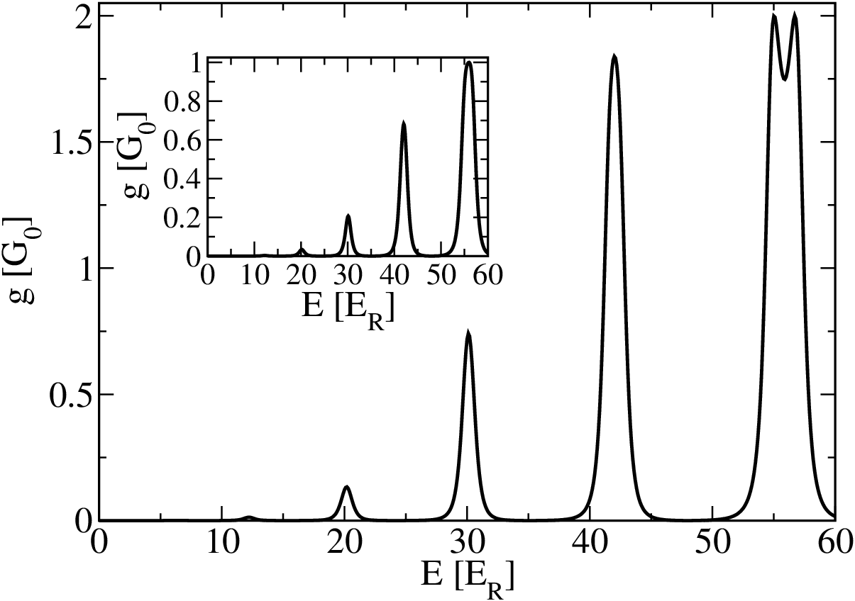
The currents transmitted through the ring carry hole polarization, as can be seen from the figures. The peak in the unpolarized conductance near the energy is split, while the polarized conductance shows a single peak of roughly half the height. The components of the split peak correspond to pseudospin components with high polarization up and down, described by pseudospin density matrices (30) with and . This splitting is a clear signature of pseudospin dependent transport.
The standard setup for a study of conductance oscillations as a function of the magnetic field consists of measuring the conductance at a fixed lead chemical potential and sweeping the external magnetic field. The conductance then typically reveals the oscillations with the period , being the ring surface area and the flux quantum. The spin-orbit coupling was found to modify these oscillations [15]. In our model the conductance is modified due to the presence of four closely spaced energy levels that correspond to each peak in the conductance. At zero flux these four levels are the Kramers doublets and . The splitting between these pairs in the absence of magnetic field is of second order in spin-orbit coupling. As the magnetic flux is threaded through the ring the quartet of levels splits, with two of the levels with gaining energy, and the levels with losing it. In addition the Zeeman coupling splits these levels further. This behavior is in sharp contrast to the linear spin-orbit coupling case where there are at most two states of any given energy.
The four-peak structure within the maximum of conductance in Aharonov-Bohm oscillations represents a signature of the cubic spin-orbit coupling, see Fig. 9. The period of oscillations is equal for both types of coupling, but the shape of the peaks is drastically different.

The four-peak structure is most visible when the leads are tuned into the vicinity of a ring energy level. At these energies, in contrast, the linear spin-orbit coupling produces a single-peak structure.
Fourier spectra of conductance fluctuations were reported to show the signature of spin-orbit coupling in the diffusive regime, seen in the splitting of peaks in the Fourier spectrum [15, 16]. We have compared the Fourier spectra of our results in the case of linear and cubic form of spin-orbit coupling. In our tunneling model, the Fourier spectra of the ring with linear spin-orbit coupling differs from the spectra of the ring with the cubic spin-orbit coupling in the relative size of the base and higher harmonic. The shape of the peaks in Fourier spectrum does not show significant differences.

Therefore, the signature of the cubic spin-orbit coupling is clearly visible in the direct-space Aharonov-Bohm oscillations, and very hard to discern in the Fourier transform.
V.4 Thermal broadening
The split peaks in differential conductance as function of lead chemical potential will be visible is the distance between the peaks is larger then their width. As an illustration of the effects of temperature , we will investigate the broadening of pseudospin-resolved peak at half flux quantum , Fig. 11. For the parameters we used, the splitting of the peaks is , and requires low temperatures to resolve. The broadening that impairs resolving of the split peaks has a temperature-independent contribution due tunneling to the leads, and it is further increased due to the temperature. We study the thermal broadening of the conductivity using (26), and finding the conductance at finite temperatures. We find that the conductance is indeed broadened at finite temperatures, Fig. 11. However, the visibility of the peaks and the resolution of peaks can be improved if the peaks are narrower or the splitting is larger. The peak splitting grows with the absolute value of the momentum, , and can be observed at higher temperatures if the momentum of the interfering states is larger. In summary, the favorable conditions for the observation of pseudospin- dependent conductance are weak tunneling and low temperatures. Both of these conditions aim at reducing the line width of the peaks. Another way to resolve the pseudospins is to perform an experiment with the higher chemical potential in the leads, and observe the splitting of the higher-energy peak. These peaks are further separated in energy, due to the cubic spin orbit coupling.

VI Conclusions
We have investigated the conductance of a mesoscopic ring of heavy holes tunnel-coupled to leads. In the coherent regime, the transport through the ring is dominated by the the energy spectrum and the pseudospin texture of the orbiting hole eigenstates. Due to the cubic form of spin-orbit interaction, the pseudospin texture of the hole eigenstates is momentum dependent, as opposed, e.g., to the electrons with linear spin-orbit coupling.
The hole transport proceeds through tunneling between the source and the drain lead via various ring eigenstates, with the phase of each tunneling path modified due to the spin texture. The effects of interference between the tunneling paths are visible in the conductance when the tunnel broadening is sufficient to make the ring energy levels overlap. We have demonstrated that the dominant type of spin-orbit interaction can be deduced from the pseudospin-dependent conductance between the polarized leads.
Aharonov-Bohm oscillations appear in the tunneling approach as a consequence of the evolution the ring spectrum as the magnetic flux is threaded through the ring. Approximately periodic evolution of the peaks leads directly to the approximately periodic conductance oscillations. We have explained the four-peak shape of the Aharonov-Bohm oscillations in the direct space as a direct consequence of four-fold near degeneracy of the orbiting hole energy levels. This particular shape of Aharonov-Bohm oscillations is a signature of the cubic spin-orbit coupling, but it is not visible in the Fourier transform of the conductance.
The pseudospin splitting of the conductance peaks, caused by pseudospin textures of the ring eigenstates is clearly visible at zero temperature and low tunneling, but disappears when the combined thermal- and tunnel broadening becomes comparable to the size of the splitting.
We thank M. Trif, J. C. Egues, and C. Bruder for useful discussions. We acknowledge financial support from the Swiss SNF, the NCCR Nanoscience Basel; the EU under “MagMaNet”, and “MolSpinQIP”, Brain Korea 21 Project, DFG within SPP 1285 “Spintronics” and FOR 921.
References
- [1] Y. Aharonov and D. Bohm, Phys. Rev. 115, 485 (1959).
- [2] Y. Aharonov and A. Casher, Phys. Rev. Lett. 53, 319 (1984).
- [3] M. Lee and M. Y. Choi, Journal of Physics A: Mathematical and General 37, 973 (2004).
- [4] M. F. Borunda, X. Liu, A. A. Kovalev, X.-J. Liu, T. Jungwirth, and J. Sinova, arXiv:0809.0880 (2008).
- [5] T. Bergsten, T. Kobayashi, Y. Sekine, and J. Nitta, Phys. Rev. Lett. 97, 196803 (2006).
- [6] M. Pletyukhov and U. Zülicke, Phys. Rev. B 77, 193304 (2008).
- [7] C. P. Umbach, S. Washburn, R. B. Laibowitz, and R. A. Webb, Phys. Rev. B 30, 4048 (1984).
- [8] O. Entin-Wohlman, Y. Imry, and A. Aharony, Phys. Rev. Lett.91, 046802 (2003).
- [9] D. Loss, P. Goldbart, and A. V. Balatsky, Phys. Rev. Lett. 65, 1655 (1990).
- [10] D. Loss and P. M. Goldbart, Phys. Rev. B 23, 13544 (1992).
- [11] J. Nitta, F. E. Meijer, and H. Takayanagi, App. Phys. Lett.75, 695 (1999).
- [12] R. Citro, F. Romeo, and M. Marinaro, Phys. Rev. B 74, 115329 (2006).
- [13] R. Citro and F. Romeo, Phys. Rev. B 75, 073306 (2007).
- [14] R. Citro and F. Romeo, Phys. Rev. B 77, 193309 (2008).
- [15] B. Grbic, R. Leturcq, T. Ihn, K. Ensslin, D. Reuter, and A. D. Wieck, Phys. Rev. Lett. 99, 176803 (2007).
- [16] B. Habib, E. Tutuc, and M. Shayegan, App. Phys. Lett. 90, 152104 (2007).
- [17] M. G. Pala, M. Governale, J. König, and U. Zülicke, Europhys. Lett. p. 850 (2004).
- [18] H.-A. Engel and D. Loss, Phys. Rev. Lett. 93, 136602 (2004).
- [19] A. A. Kovalev, M. F. Borunda, T. Jungwirth, L. W. Molenkamp, and J. Sinova, Phys. Rev. B 76, 125307 (2007).
- [20] S. Souma and B. K. Nikolić, Phys. Rev. B 70, 195346 (2004).
- [21] W. Hofstetter, J. König, and H. Schoeller, Phys. Rev. Lett. 87, 156803 (2001).
- [22] J. König and Y. Gefen, Phys. Rev. B 65, 045316 (2002).
- [23] P. Simon, O. Entin-Wohlman, and A. Aharony, Phys. Rev. B 72 (2005).
- [24] D. Loss, H. Schoeller, and P. M. Goldbart, Phys. Rev. B 48, 15218 (1993).
- [25] Y.-B. Yau, E. P. De Poortere, and M. Shayegan, Phys. Rev. Lett. 88, 146801 (2002).
- [26] D. V. Bulaev and D. Loss, Phys. Rev. Lett. 95, 076805 (2005).
- [27] F. E. Meijer, A. F. Morpurgo, and T. M. Klapwijk, Phys. Rev. B 66, 033107 (2002).
- [28] B. Molnár, F. M. Peeters and P. Vasilopoulos, Phys. Rev. B 69, 155335 (2004).
- [29] U. Fano, Phys. Rev. 124, 1866 (1961).
- [30] D. Averin, J. Appl. Phys. 73, 2593 (1993).
- [31] H. Haug and A.-P. Jauho, Quantum Kinetics in Transport and Optics of Semiconductors (Springer, 1996).
- [32] Y. Meir and N. S. Wingreen, Phys. Rev. Lett. 68, 2512 (1992).