Wide spread spectrum watermarking with side information and interference cancellation

As seen in the introduction, the watermarking problem can be seen as a communication process with side information available at the encoder [3]. This kind of channel have been studied by Costa [4], which leaded to an upper bound of capacity for this kind of channel.

Let us consider a $n$-long i.i.d. Gaussian host signal $\underline{\mathbf{x}}$, whose samples are modeled by $X\sim{\mathcal{N}}(0,Q)$. This signal is perfectly known during the embedding process. We transmit our data with a watermark signal $\underline{\mathbf{w}}=\left\{w_{1},w_{2},\ldots,w_{n}\right\}$ as seen on Fig. 1. The energy of $\underline{\mathbf{w}}$ is bounded so that

The transmitted signal is then $\underline{\mathbf{y}}=\underline{\mathbf{x}}+\underline{\mathbf{w}}$. This signal is corrupted during the transmission by an added Gaussian noise $\underline{\mathbf{z}}$, modeled by $Z\sim{\mathcal{N}}(0,N)$. Receiver then gets the signal $\underline{\mathbf{y}}^{\prime}=\underline{\mathbf{y}}+\underline{\mathbf{z}}$. If we consider this channel as a classical Gaussian one, two noises are added to the transmitted signal, so the capacity is given by

Side information $\underline{\mathbf{x}}$ impacts on the performance of the system, lowering the capacity. Costa showed that the side information does not influence the optimal capacity of the channel, i.e.

Ha gave a theoretical method to reach this value. He considered a signal $U\sim{\mathcal{N}}(0,P+\alpha^{2}Q)$, know both from the embedder and the extractor. The capacity of the channel is then given by

where $Y\sim{\mathcal{N}}(0,Q+P)$ models the transmitted signal $\underline{\mathbf{y}}$. Costa showed that the previous equation leads to the optimal value $\alpha=P/(P+N)$, and then to Eqn. 3. The signal $U$ is obtained using a structured codebook of $2^{n\left(I(U;Y)-\epsilon\right)}$ elements²² 2 With $\epsilon$ chosen to be very small as $n\rightarrow\infty$., designed to be a surjective function between the set of possible messages to embed ${\mathcal{M}}$ and the codebook ${\mathcal{U}}$: each possible message $\underline{\mathbf{m}}$ is associated to a sub-codebook ${\mathcal{U}}_{\underline{\mathbf{m}}}$ composed of $2^{nI(U;X)}$ codewords. During the embedding process, the closest codeword $\underline{\mathbf{u}}^{\star}\in{\mathcal{U}}_{\underline{\mathbf{m}}}$ is chosen. The watermark signal is then given by

Whereas classical watermarking techniques would have transmitted $\underline{\mathbf{x}}+\sqrt{nP}\times\underline{\mathbf{u}}^{\star}/\|\underline{\mathbf{u}}^{\star}\|$, the $\alpha$ term forces the transmitted signal to go toward the codevector, as illustrated by Fig. 2. At the extraction process, the closest codeword $\widehat{\underline{\mathbf{u}}}\in{\mathcal{U}}$ is computed. The decoded message is then $\widehat{\underline{\mathbf{m}}}$ so that $\widehat{\underline{\mathbf{u}}}\in{\mathcal{U}}_{\widehat{\underline{\mathbf{m}}}}$.

The original ICS is based on large random codebooks: the only way to decode $\underline{\mathbf{y}}^{\prime}$ is by an exhaustive search in ${\mathcal{U}}$. Some practical but suboptimal approaches, inspired by the ICS, have been proposed for i.i.d. Gaussian host signals, based on codebooks used for error correcting codes (ECC) [14, 5, 15, 16], where decoding process is designed to be much more simpler than an exhaustive search.

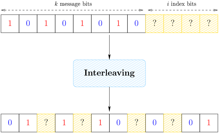
Each possible $k$-long message is associated to $2^{nI(U;X)}$ codewords. A simple way to design such a structured codebook would be to insert $i=n\times I(U;X)$ index bits in the message and to encode it. For an ECC with rate $r$, this leads to $n$-long codewords with $n=(k+i)/r$ (see Fig. 3). According to Costa, the value of $i$ is given by

which then depends on $Q$, i.e. the host signal. Thus the final codeword length $(k+i)/r$ may vary, while the host signal length $n$ is generally given and fixed (number of pixels for an image, sample size of a sound…). The length of codewords must not depend on $i$, i.e. the global rate $k/n$ must be fixed.

We thus propose to use a simple codebook based on punctured convolutional codes and soft trellis decoding. Let us choose an error correcting code in order to get a rate $r=k/n$. We then design an interleaved pattern composed of the $k$ bits from the message $\underline{\mathbf{m}}$ to be embedded and of $i$ additional bits, as illustrated in Fig. 4(a). We then expand the host signal from $n$ to $(k+i)/r$ using neutral values for soft decoding (i.e. $0$). This expanded host signal is decoded with a modified soft Viterbi decoding algorithm, using the previous $k$ bits pattern as a strong a priori in order to force some transitions in the convolutional trellis (see Fig. 4(b)). The output fixes the $i$ index bits and gives a $(k+i)/r$-long codeword, which is punctured according to the previous expansion of the host signal, in order to remove $i/r$ bits and to finally get a $n$-long codeword. This leads to the closest codeword $\underline{\mathbf{u}}^{\star}\in{\mathcal{U}}_{\underline{\mathbf{m}}}$ to $\underline{\mathbf{x}}$. Using BPSK³³ 3 Binary Phase Shift Keying., all the obtained codewords are designed to have the same energy, i.e. $\|\underline{\mathbf{u}}\|=\sqrt{n}$.

The watermark is finally chosen in order to get the maximum robustness [17]: the codeword $\underline{\mathbf{u}}^{\star}$ is associated to a hyper-cone of robustness, where $\underline{\mathbf{y}}$ must lie into to be correctly decoded. Further, hyperboloids may be defined to represent set of points of given robustnesses (e.g. ${\mathcal{H}}_{N_{1}}$, ${\mathcal{H}}_{N_{2}}$…on Fig. 2). The watermark $\underline{\mathbf{w}}$ is defined in order to maximize robustness, that is

where $\theta$ is the angle of the hyper-cone, given by [13]

At the receiver, the signal $\underline{\mathbf{y}}^{\prime}=\underline{\mathbf{y}}+\underline{\mathbf{z}}$ is expanded from $n$ to $(k+i)/r$ elements insertion $0$ elements, and decoded using the trellis to get $\underline{\mathbf{m}}$. Thanks to soft decoding and to the fact that codewords have all same energy, this coding scheme is scale resistant, i.e. $\underline{\mathbf{y}}^{\prime}$ can be scaled ($\underline{\mathbf{y}}^{\prime}=\gamma\left[\underline{\mathbf{y}}+\underline{\mathbf{z}}\right]$ with $\gamma>0$) without loss of robustness.

Multimedia signals are not usually i.i.d. and Gaussian. So we consider a non i.i.d. host signal $\underline{\mathbf{x}}$ modeled by a set of random variables $X^{m}=\left\{X_{1},X_{2},\ldots,X_{m}\right\}$ with $X_{i}\sim{\mathcal{N}}(0,\sigma_{X_{i}}^{2})$, i.e. signal is modeled as a mixture of Gaussians. We also consider a more general model for attack: SAWGN. The received signal can then be written as $y^{\prime}_{i}=\gamma_{i}^{\textrm{a}}\times y_{i}+z_{i}$ where $\gamma_{i}^{\textrm{a}}\geq 0$ and $z_{i}$ is a Gaussian noise modeled by $Z_{i}\sim{\mathcal{N}}(0,\sigma_{Z_{i}}^{2})$. To embed a $n$ symbols length message in a $m$-long signal, wide spread spectrum uses a pseudo-random matrix $\underline{\mathbf{G}}\in\left\{-1;1\right\}^{m\times n}$. This can be associated to a spread transform, i.e. the embedding process is made in a linear subspace, like for ST-DM [15] or ST-SCS [18, 9]. Our previous work [12, 19] demonstrated the interest of Wiener filtering at embedding⁴⁴ 4 Since attacker would perform Wiener filtering to decrease $D_{xy^{\prime}}$, Wiener filtering at embedding allows to decrease $D_{xy}$ without loss of performance.:

The watermark $\underline{\mathbf{w}}=\left\{w_{1},w_{2},\ldots,w_{m}\right\}$ is thus non i.i.d. and is modeled by $W^{m}$ with $W_{i}\sim{\mathcal{N}}(0,\sigma_{W_{i}}^{2})$. The Wiener filtering and the scale attack can be grouped: $\gamma_{i}=\gamma_{i}^{\textrm{a}}\times\gamma_{i}^{\textrm{w}}$. The inverse spread transform (used for extraction) is defined by a weighted linear correlation [12]:

where $\beta_{i}$ is a weighting factor. As demonstrated previously [13] considering a SI scheme, the optimal value for $\beta_{i}$ can be expressed as

In this subspace, the embedding process from Eqn. (9) is written as

where $\underline{\mathbf{x}}^{\textrm{st}}$ is i.i.d. and Gaussian. We can then use Costa’s approach described in Sec. 2.1, and define from Eqns. (9) and (12) the different amounts of energy used as

We remark that while $\sigma_{X_{i}}^{2}\gg\sigma_{W_{i}}^{2}$ to ensure the invisibility of the watermark, the available watermark energy $P$ is concentrated in the subspace and can then become more important than the energy $Q$ of the host signal (when $m/n\gg 1$). It also shows that $P$ is shared by the symbols to be embedded: more symbols (i.e. larger $n$) means less watermark energy per symbol.

Given a maximum amount of embedding distortion, we must optimize the embedding energy, i.e. $\sigma_{W_{i}}$. Define an embedding and an attack distortion functions:

where $\varphi_{i}$ is a perceptual weighting factor. The performance of the inverse spread transform can be quantified by the signal-to-noise ratio $E_{b}/N_{0}$ defined as

It should be noted that this value is not the signal-to-noise ratio obtained at the output of the extractor from Eqns. (12) and (13), given by [13]

We now solve the optimization of $\sigma_{W_{i}}$ using a min-max game: given a maximal amount of distortion $D_{xy^{\prime}}^{\max}$, the attacker wants to minimize $E_{b}/N_{0}$, while the embedder wants to maximize it, for a maximal amount of embedding distortion $D_{xy}^{\max}$. This is done by two Lagrangian optimizations [12]. First, for the attacker, we get the following functional:

where $\lambda$ is a Lagrangian multiplier used to respect the constraint on the attack distortion. This leads to the optimal values for $\gamma_{i}$ and $\sigma_{Z_{i}}$:

The second part of the game consists in optimizing the embedding parameters considering optimal attack, which is also done by a Lagrangian approach:

where $\chi$ is a Lagrangian multiplier used to respect the constraint on the embedding distortion. This leads to the final optimal embedding parameters

and also to a particular expression for the optimal correlation factor for inverse spread transform: $\beta_{i}^{\star}\propto\varphi_{i}$, when considering optimal attacks.

To avoid interference, a trick is to embed only one symbol per host element [15], i.e. $\forall i\in\left\{1,2,\ldots m\right\}$, there is only one element in $\left\{G_{i,1},G_{i,2},\ldots,G_{i,n}\right\}$ which is not set to $0$. In this case, $I=0$. However this technique limits the spreading of the bits, especially for important values of $n$, case where interference cancellation is very interesting (low level of attack noise).

Moreover, in the case of smooth signals (see Fig. 6 for an example), the number of well suited host elements (important value of $\gamma_{i}\sigma_{W_{i}}/\sigma_{X_{i}}$) is limited. The energy of the watermark is mainly located on high energy coefficients. Since this number of coefficients is small, symbols to be hidden may not be equally spread over the host signal (i.e. a symbol may be spread on non significant coefficients whereas an other one will be spread on significant ones). It results in the linear subspace in non i.i.d. signals. Performances are not guaranteed and parallel channels should rather be considered.

If pseudo-random carriers were used at embedding, the received signal in the spread transform subspace can be written as

where $\textsf{isi}(\underline{\mathbf{w}}^{\textrm{st}})$ is the inter-symbols interference. For $Q\ll P$ (very common case for payloads such as $n<1000$), we can write $\underline{\mathbf{x}}^{\textrm{st}}+\underline{\mathbf{w}}^{\star}\simeq\underline{\mathbf{w}}^{\textrm{st}}\simeq\sqrt{P}\times\underline{\mathbf{u}}^{\star}$ and then

Thus we can estimate $\textsf{isi}(\sqrt{P}\times\underline{\mathbf{u}}^{\star})$ in order to cancel ISI. Receiver first estimates $\underline{\mathbf{u}}^{\star}$. Corresponding interference is then canceled. The new $\underline{\mathbf{y}}^{\prime\textrm{st}}$ is obtained and used to compute $\widetilde{\underline{\mathbf{u}}}^{\star}$. This process iterates until $\underline{\mathbf{u}}^{\star}=\widetilde{\underline{\mathbf{u}}}^{\star}$ (see Alg. 1). To be efficient, receiver must know (or estimate) embedding energy $\sigma_{W_{i}}$. Moreover, optimal scaling factor $\gamma_{i}^{\star}$ must also be estimated. This may be done by an additional reference signal, leading to a lower capacity for message bits. We will then search for another solution consisting in canceling ISI at embedding.

As seen in Sec. 2.1, the use of the side information available during the embedding process leads to great improvements, and if no attack is applied during the transmission, the capacity of the channel is infinite. But the spread transform we use to embed the watermark introduces a noise that limits capacity due to ISI. We propose to consider ISI as a kind of side information.

Even if this interference is introduced by the embedder, it is not perfectly known before the embedding. So, it can not be directly considered as side information. The problem is that the interference depends on the watermark signal, which depends on the interference. We use an iterative algorithm to converge to a watermark signal that takes into account its own interference. This algorithm is described by Alg. 2. We first compute $\underline{\mathbf{w}}^{\textrm{st}}$, as explained in Sec. 2. The interference it produces is computed, and introduced as side information. In a second step, this new side information $\widetilde{\underline{\mathbf{x}}}^{\textrm{st}}$ is used to compute an updated watermark signal. The previous steps are iterated until $\underline{\mathbf{w}}^{\textrm{st}}$ converges (we observe convergence is attained to after typically less than 3 iterations). At the end of the loop, the watermark signal takes into account the host signal and the symbol interference, and is added using Eqn. (9).

References

- [1] S. D. Servetto, C. I. Podilchuk, and K. Ramchandran, “Capacity issues in digital image watermarking,” in Proc. Int. Conf. on Image Processing, 1, pp. 445–449, (Chicago, IL), Oct. 1998.
- [2] P. Moulin and J. A. O’Sullivan, “Information-theoretic analysis of information hiding,” IEEE Trans. on Info. Thy , Oct. 1999.
- [3] I. J. Cox, M. L. Miller, and A. L. McKellips, “Watermarking as communications with side information,” Proc. IEEE 87, pp. 1127–1141, Jul. 1999.
- [4] M. H. M. Costa, “Writing on dirty paper,” IEEE Trans. Info. Thy 29, pp. 439–441, May 1983.
- [5] J. J. Eggers, J. K. Su, and B. Girod, “A blind watermarking scheme based on structured codebooks,” in Proc. IEE Colloq.: Secure Images and Image Authentification, (London, UK), Apr. 2000.
- [6] J. Chou, S. S. Pradhan, L. E. Ghaoui, and K. Ramchandran, “A robust optimization solution to the data hiding problem using distributed source coding principles,” in Proc. SPIE, 3974, Jan. 2000.
- [7] J. K. Su, J. J. Eggers, and B. Girod, “Analysis of digital watermarks subjected to optimum linear filtering and additive noise,” IEEE Trans. Signal Proc.: Special Issue on Information Theoretic Issues in Digital Watermarking 81, Jun. 2001.
- [8] P. Moulin and A. Ivanovic, “The watermark selection game,” in Proc. Conf. on Info. Sciences and Systems, Mar. 2001.
- [9] J. J. Eggers, R. Bäuml, and B. Girod, “Digital watermarking facing attacks by amplitude scaling and additive white noise,” in 4th Int. ITG Conf. on Source and Channel Coding, Jan. 2002.
- [10] P. Moulin, “The parallel-Gaussian watermarking game,” in Proc. 35th Conf. on Information Sciences and Systems, (Baltimore, MD), Mar. 2001.
- [11] A. S. Cohen and A. Lapidoth, “The Gaussian watermarking game,” IEEE Trans. Info. Thy , Jun. 2002.
- [12] G. Le Guelvouit, S. Pateux, and C. Guillemot, “Perceptual watermarking of non i.i.d. signals based on wide spread spectrum using side information,” in Proc. Int. Conf. on Image Processing, (Rochester, NY), Sep. 2002.
- [13] S. Pateux and G. Le Guelvouit, “Practical watermarking shceme based on wide spread spectrum and game theory,” To appear in Signal Processing: Image Communication , 2003.
- [14] M. Ramkumar and A. Akansu, “A capacity estimate for data hiding in Internet multimedia,” in Symp. on Content Security and Data Hiding in Digital Media, (Newark, NJ), May 1999.
- [15] B. Chen and G. W. Wornell, “Quantization index modulation: a class of provably good methods for digital watermarking and information embedding,” IEEE Trans. Info. Thy 47, pp. 1423–1443, May 2001.
- [16] J. Chou, S. S. Pradhan, and K. Ramchandran, “Turbo coded treillis-based constructions for data embedding: channel coding with side information,” in Proc. Conf. on Signals, System and Computers, (Asilomar, CA), Nov. 2001.
- [17] M. L. Miller, I. J. Cox, and J. A. Bloom, “Informed embedding: exploiting image and detector information during watermark insertion,” in Proc. Int. Conf. on Image Processing, (Vancouver, Canada), Sep. 2000.
- [18] J. J. Eggers, J. K. Su, and B. Girod, “Performance of a practical blind watermarking scheme,” in Proc. SPIE, (San Jose, CA), Jan. 2001.
- [19] G. Le Guelvouit, S. Pateux, and C. Guillemot, “Information-theoretic resolution of perceptual WSS watermarking of non i.i.d. Gaussian signals,” in Proc. Eur. Signal Processing Conf., 1, pp. 454–457, (Toulouse, France), Sep. 2002.
- [20] A. B. Watson, “DCT quantization matrices visually optimized for individual images,” Proc. SPIE 1913, pp. 202–216, 1993.