Interaction and excitonic insulating transition in graphene
Abstract
The strong long-range Coulomb interaction between massless Dirac fermions in graphene can drive a semimetal-insulator transition. We show that this transition is strongly suppressed when the Coulomb interaction is screened by such effects as thermal fluctuation, doping, disorder, and finite volume. It is completely suppressed once the screening factor is beyond a threshold even for infinitely strong coupling. However, such transition is still possible if there is an additional strong contact four-fermion interaction. The differences between screened and contact interactions are also discussed.
pacs
73.43.Nq, 71.10.Hf, 71.30.+hThe low-energy elementary excitations in undoped graphene are massless Dirac fermions. Their spectral and transport properties are quite unusual and have attracted intense investigations in the past several years [1, 2]. For a clean undoped graphene, the density of states (DOS) vanishes linearly near the Dirac point. As a result, the Coulomb interaction between massless Dirac fermions is essentially unscreened, in sharp contrast to the electron system with parabolic dispersion. The unscreened, long-range Coulomb interaction was shown to be responsible for many anomalous behaviors of graphene [3, 4, 5, 6, 7, 8, 9, 10, 11].
At the strong coupling regime, the long-range Coulomb interaction can open a finite mass gap for the Dirac fermion, which then drives a phase transition from the semimetal state to an insulator state. This transition is realized by forming stable particle-hole pairs and usually named as excitonic semimetal-insulator (SM-IN) transition [4, 5]. Recently, this kind of phase transition has been studied by nonperturbative Dyson-Schwinger (DS) equation approach [4, 5, 6], renormalization group method [9], and lattice simulations [12, 13]. The SM-IN transition was found in graphene for strong Coulomb coupling and small fermion flavor [4, 5]. The effects of finite temperature and external magnetic field were also considered [5].
Although being of remarkable interests, the predicted SM-IN transition (in zero magnetic field) has not yet been unambiguously observed in experiments. In this paper, we discuss the effects that can potentially prevent the appearance of this SM-IN transition. First of all, it should be emphasized that such transition can take place only for strong, poorly screened Coulomb interaction. Generically, there are two critical parameters: critical dimensionless coupling strength and critical fermion flavor . SM-SI transition is possible only when and . Once the long-range Coulomb interaction is screened by some physical effects, there will be an effective screening factor , which is expected to increase and reduce . This can be understood by noting the important fact that SM-SI transition realized by forming fermion-antifermion pairs is a genuine low-energy phenomenon. From the experience in QED3, the long-range nature of gauge interaction plays the crucial role in generating the dynamical mass gap for initially massless Dirac fermions [14]. A finite gauge boson mass rapidly reduces the critical fermion flavor to below the physical value [14]. In the present case, there is a similar suppressing effect once the long-range Coulomb interaction is screened for some reason. The opening of excitonic gap requires that the Coulomb interaction is sufficiently strong at low-momentum region. However, the screening factor suppresses the contribution from small momenta significantly. Obviously, this kind of pairing instability is markedly different from the conventional BCS-type pairing formation, which is caused by arbitrary weak attractive force between electrons.
In realistic graphene samples, the critical behavior of SM-IN transition can be influenced by the following reasons: thermal fluctuation; doping; disorder; finite sample volume. Each of them can generate an effective screening factor , which could be regarded as an effective photon mass. We study their effects on critical strength and critical flavor by solving the corresponding gap equation, and show that a growing significantly increases and reduces , both at zero and finite temperatures. When is beyond some threshold , the excitonic transition is completely prohibited, leaving semi-metal as the stable ground state. Frequently, some of these effects coexist, leading to further suppression of excitonic transition. However, even when , we found that the excitonic transition can still take place if there is an additional strong contact quartic interaction. We also briefly discuss the interesting differences between the screened Coulomb and contact quartic interactions.
The total Hamiltonian of massless Dirac fermion is given by
Here, we adopt four-component spinor field to describe the massless Dirac fermion since there is no chiral symmetry in the two-component representation. The conjugate spinor field is defined as . The -matrices satisfy the standard Clifford algebra. Although the physical fermion flavor is actually , in the following we consider a large in order to perform expansion. The total Hamiltonian preserves a continuous U(2N) chiral symmetry , which will be dynamically broken if a nonzero fermion mass gap is generated.
The free propagator of massless Dirac fermion is . The Coulomb interaction modifies it to the complete propagator
| (1) |
where denotes the dynamical fermion mass and the wave function renormalization functions. To the leading order in expansion, the DS integral equation is
| (2) |
where the vertex function has already been approximated by the bare matrix . The nontrivial solution of this equation signals the opening of an excitonic gap.
In the DS gap equation, is the Coulomb interaction function. The bare, unscreened Coulomb interaction has the form in the momentum space. For an interacting electron gas, the collective density fluctuations screen the bare Coulomb interaction to . For ordinary non-relativistic electron gas, the static polarization function is just the zero-energy DOS, , which is known to be finite. The parameter defines the inverse Thomas-Fermi screening length. The case for undoped clean graphene is quite different because of the linear dispersion of Dirac fermions. The leading contribution to polarization function is given by . It vanishes linearly as in the static limit , so the long-range Coulomb interaction is unscreened.
Under the approximations described above, the gap equation can be written as
| (3) |
with interaction function
| (4) |
Here, is assumed and the rescaling , is made (such rescaling will be made throughout the whole paper). The present problem contains two parameters: fermion flavor and dimensionless Coulomb coupling defined as , where . The ultraviolet cutoff is taken to be of order eV which is determined by with lattice constant . Not that no instantaneous approximation for the polarization function is made at present. We solve the nonlinear gap equation using bifurcation theory and parameter embedding method [14, 15] for a number of fixed values of . The fermion flavor serves as the embedded parameter in seeking the bifurcation point. The results are shown in Fig. 1(a). It is easy to see that the critical flavor is an increasing function of . For , ; for , .
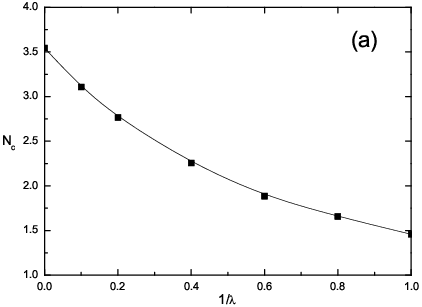

The above results are valid only for the unscreened Coulomb interaction at zero temperature. In realistic systems, the long-range interaction could be screened by several physical effects, such as thermal fluctuation, doping, disorder, and finite volume. If the polarization function takes a finite value due to some mechanism in the and limit, then the long-range Coulomb interaction becomes short-ranged and defines the screening factor. Before computing by taking each screening effect into account, we now phenomenologically introduce a single parameter (in unit of eV) to model the screened interaction function
| (5) |
The advantage of this parameter is that it explicitly measures the suppressing effect on the critical behavior due to all possible screening mechanisms. If we regard this function as the effective interaction strength, then the influence of becomes clear: it eliminates the contribution of small momenta to the gap equation Eq. (3). But remember that the excitonic gap generation is primarily determined by the contribution from this region, so it is expected that a large will destroy SM-IN transition. After solving the gap equation, we found that a growing leads to increase of critical strength and to decrease of critical flavor (see Fig. 2(a)). Beyond some critical value , the SM-IN transition is completely prevented, even when the dimensionless strength .
The possible screening mechanisms will be discussed in order. First of all, the thermal fluctuation will surely restore the chiral symmetry even it is broken by the ground state. At finite temperatures, the Matsubara fermion propagator is
| (6) |
where is the fermion frequency. Here, in order to carry out the frequency summation appearing in the gap equation, we utilize the instantaneous approximation [4, 5]. Under this approximation, the polarization function can be approximated [16] by
| (7) |
with constant . At the limit , the polarization is , corresponding to the thermal screening factor . Since other screening effects can coexist with thermal fluctuations at finite temperatures, we still introduce the parameter and write the gap equation as
| (8) | |||||
with the interaction function
| (9) |
The results at finite temperatures are rather complex since now we have four parameters, , , , , each of which has a critical value. Their relationships are shown in Fig. 1(b) without screening effects () and in Fig. 2(b) with screening (the temperature is in unit of ). In Fig. 2(b), the Coulomb coupling parameter is fixed at , and the results for other values of are not shown since they are qualitatively similar. The results tell us that the thermal suppression is more important than screening effect when has small values (), but the screening effect eventually becomes much more important than thermal effect for larger values of .


The second potential mechanism that can prevent gap generation is doping. The Coulomb interaction between Dirac fermions is unscreened only when the graphene is undoped. When the graphene is slightly doped, the finite carrier density then serves as an effective screening factor . Then the excitonic gap is expected to open only at or very close to the Dirac point. The critical carrier density has been discussed previously in [5]. Recently, the same screening effect was emphasized in the study of exciton condensate in bilayer graphene [17]. At finite chemical potential , the fermion propagator becomes
| (10) |
Using this propagator, the polarization function can be calculated with the result
| (11) | |||||
in the zero frequency limit. As , , which defines the screening factor . After performing the frequency summation, the gap equation has the form
with the interaction function being
| (12) |
Note the chemical potential appears in two places: the occupation number and the polarization function. To see the dominant effect of , we first solved the full gap equation and show the results in Fig. 3(a) (also at for comparison). The dependence of on and qualitatively resembles that in Fig. 2(b), but visibly exhibits different quantitative behavior: the suppressing effect from doping is more prominent at low than at higher . Despite the details, a large doping makes the excitonic insulating state impossible. Then we solved the gap equation by ignoring the -dependence of occupation number and found that the results are nearly the same as Fig. 3(a) (therefore not shown). It seems that the screening effect induced by doping plays the dominant role in suppressing the gap generation.
Next, we consider the influence of disorders, which are unavoidable in graphene samples. The disorders can be crudely classified as random mass, random chemical potential, and random vector potential, etc, and have been extensively treated using various field theoretic techniques [18, 19, 20, 21, 22]. The low-energy DOS was found to be sensitive to the symmetry of disorders [20, 21, 22]. For instance, random vector potential leads the DOS to vanish algebraically upon approaching the Fermi surface with exponent depending on symmetry [20, 22]. For this kind of disorder, there is essentially no screening effect and the Coulomb interaction remains long-ranged, provided that the Altshuler-Aronov type correction to low-energy DOS is not included. For random mass potential, the zero-energy DOS can have finite value, as a result of dynamical discrete symmetry breaking [18, 21]. In the case of weak disorders, the impurity scattering can be treated within the conventional self-consistent Born approximation, which reveals that the zero-energy DOS acquires a finite value of the form [19], , with a constant scattering rate . The finite screens the long-range Coulomb interaction. Within the Matsubara formalism, such screening effect can be elaborated by including the scattering rate into the polarization function.


To study the role of weak disorders, we first write the effective Dirac fermion propagator
| (13) |
which contains the scattering rate . Due to the sign dependence of scattering rate, the gap equation and polarization function becomes rather complicated. After frequency summation within the instantaneous approximation, the gap equation is found to be
| (14) | |||||
where is the digamma function. At the clean limit, , the imaginary part of digamma function can be simplified as which is the same as that appearing in gap equation Eq. (8). As in the case of chemical potential, the screening effect caused by disorder scattering can be directly seen by calculating the vacuum polarization function and then taking the limit. However, even in the instantaneous approximation, it is not easy to obtain the complete form of . When the scattering rate is larger than the thermal scale , , we found that the polarization function can be well approximated by the following expression(as detailed in Appendix)
| (15) |
with constant . At the limit , it takes a finite value
| (16) |
which is proportional to the scattering rate and defines the screening factor. Comparing the polarization Eq. (15) with Eq. (7), formally the scattering rate plays the role of an effective temperature . Now the interaction function in gap equation Eq. (14) becomes
| (17) |
On the other hand, in the case of small the polarization function should be replaced by Eq. (7). After solving the full gap equation Eq. (14), we present the dependence of on scattering rate for different values of in Fig. 3(b). In order to see the effects of screening on gap generation, we also solved the gap equation when appears only in the interaction function . The quantitative difference between the results in these two cases is negligible. The results in Fig. 3(b) show that there is a competition between the suppressing effects of thermal fluctuation and disorder scattering. At low temperature , the scattering rate dominates; while for small , the thermal effect dominates. Obviously, a large suppresses the possibility of gap generation rapidly. Further, we solved the gap equations Eq. (8) and Eq. (9) with the screening factor simply set to be and found that the results are quantitatively similar to Fig. 3(b).
One might argue that the low-energy fermionic excitations are all suppressed once a fermion mass gap opens, so the DOS vanishes at energy scale below the gap and there is no screening effect. However, for fermion of mass , the zero-energy DOS was found [23] to be . In principle, we might include a gap into the polarization function and then study the gap equation. Since the critical behavior of SM-IN transition is studied by linearizing the nonlinear gap equation, the mass can be safely set to zero, , near the bifurcation point.
Finally, we discuss effect of finite sample volume (area in two dimensions). For a graphene plane of finite spatial extent, the particle momenta becomes discrete and the momenta transferred in the process of interaction can not be arbitrary small. If we still work in the continuum field theoretic formalism, this effect can be equivalently represented by imposing an infrared cutoff , given by the inverse sample size . Its effects on is nearly the same as Fig. 2(a) at and Fig. 2(b) at finite with replaced by , and hence are not shown explicitly. The results imply that the sample of large spatial extent is more favorable to undergo the SM-IN transition [24].
Besides the above four effects, any other mechanism that can screen the long-range Coulomb interaction will also unavoidably lower the possibility of gap generation. If more than one screening effects coexist in reality, the suppression of SM-IN transition becomes much more significant, as shown in Fig. 2. In light of these results, we conclude that the excitonic insulating state can most probably be observed in undoped, clean graphene of large area near absolutely zero temperature.
Once the long-range Coulomb interaction is screened, one interesting question is whether it can be equivalently replaced by a short-range or even a contact (on-site) repulsive interaction [2]. This question can also be asked in another way: is the long-range nature or the strong coupling nature of Coulomb interaction more important in driving the SM-IN transition? If the answer is the latter, then the long-range interaction can well be replaced by a short-range or contact one. According to the above results, it seems that the long-range, rather than strong coupling, nature plays the dominant role. As shown in Fig. 2(a), even in the very strong coupling limit , the critical flavor is already less than the physical flavor when the screening factor . For moderately strong coupling , the excitonic insulating behavior becomes impossible even if the screening factor is only as small as .

In order to test the role of contact interaction and see its difference from the screened Coulomb interaction, we add one quartic interacting term to the Hamiltonian. There are several choices for the four-fermion coupling term, classified by the gamma matrices used to define the action [25, 26]. For simplicity, we consider only one of them, i.e.,
| (18) |
To the lowest order, this contact interaction contributes the following term
| (19) |
to the gap equation, where the dimensionless coupling is and the scaling is made as before. The whole gap equation is solved with results shown in Fig. 4 at (). The contact four-fermion interaction has opposite effect on the critical flavor as compared with the screening factor : while the latter rapidly suppresses , the former is very efficient in promoting the system towards the excitonic insulating phase (note there is no Goldstone boson in the insulating phase since the total Hamiltonian preserves discrete chiral symmetry ). Thus we see that the contact four-fermion interaction is actually different from the screened Coulomb interaction. For a relatively large screening factor , the latter is unable to generate excitonic gap even in the limit, while the former can generate such gap when its coupling is larger than some critical value . The reason for this difference can be seen from the gap equation: for screened Coulomb interaction, appearing in the denominator suppresses the contribution from large momenta, while in the denominator suppresses the contribution from small momenta; on the contrary, for contact fermion interaction, the coupling is constant in the whole momenta region without any suppressing effect. In conclusion, the SM-IN transition is still possible if there is additional strong contact fermion interaction, even when the screened Coulomb interaction itself can not open the gap.
We end with a brief discussion on the validity of the gap equation used in this paper. In a rigorous treatment, the excitonic gap generation should be studied by solving the self-consistent equations of fermion self-energy function, wave function renormalization, Coulomb interaction, and vertex function. In practice, a number of approximations must be utilized. Here we kept only the Fock diagram for the fermion self-energy and omit all higher order corrections of the expansion [4, 5]. The results should be qualitatively reliable for large . To verify the conclusions obtained in the leading order, it would be necessary to include these corrections (such as wave function renormalization, vertex function correction, etc.) since they might change the quantities of critical parameters and considerably for the physical flavor . However, this is beyond the scope of the present work. Another question concerns the important effect of velocity renormalization on the excitonic gap instability [9, 10]. This effect has been addressed recently by incorporating the momentum-dependent fermion velocity into the gap equation [27]. It was found that the velocity renormalization does not dramatically affect the excitonic instability [27].
G.Z.L. thanks D. V. Khveshchenko, T. Tu and I. L. Aleiner for helpful communications. This work was supported by the NSF of China under Grant No. 10674122.
Appendix A CALCULATION OF
In this appendix, we present the derivation of the polarization function at finite impurity scattering rate and finite temperature. The fermion contribution to the vacuum polarization is given by
| (20) |
Here and , and a new momentum variable is defined by with .
Within the instantaneous approximation , the polarization function reduces to
| (21) |
where is given by
| (22) |
In the presence of impurity scattering rate , the variable should be replaced by
| (23) |
Using the notation in Ref. [28], we define a new variable . Using the identity
| (24) | |||||
the function now becomes
| (25) | |||||
from which the function is given by . Define , and , then the polarization function is written as the following integral
| (26) |
It is hard to compute this integral analytically. For relatively large scattering rate , we found that the function can be approximated by the analytic expression
| (27) |
for (with error for and averaging error for ). Then the integration over variable can be carried out with the result
It has the similar form as Eq. (7) with playing the role of an effective ”temperature”, thus the polarization function can now be approximated by
| (29) |
where . At the clean limit, , we have
| (30) |
In this case, the polarization function is still approximated by Eq. (7).
References
- [1] A. K. Geim and K. S. Novoselov, Nat. Mater. 6, 183 (2007).
- [2] A. H. Castro Neto, F. Guinea, N. M. R. Peres, K. S. Novoselov, and A. K. Geim, Rev. Mod. Phys. 81, 109 (2009).
- [3] J. Gonzalez, F. Guinea, and M. A. H. Vozmediano, Nucl. Phys. B 424, 595 (1994).
- [4] D. V. Khveshchenko, Phys. Rev. Lett. 87, 246802 (2001); D. V. Khveshchenko and H. Leal, Nucl. Phys. B 687, 323 (2004).
- [5] E. V. Gorbar, V. P. Gusynin, V. A. Miransky, and I. A. Shovkovy, Phys. Rev. B 66, 045108 (2002).
- [6] D. V. Khveshchenko and W. F. Shively, Phys. Rev. B 73, 115104 (2006).
- [7] I. F. Herbut, Phys. Rev. Lett. 97, 146401 (2006); O. Vafek and M. J. Case, Phys. Rev. B 77, 033410 (2008).
- [8] O. Vafek, Phys. Rev. Lett. 98, 216401 (2007).
- [9] D. T. Son, Phys. Rev. B 75, 235423 (2007).
- [10] I. L. Aleiner, D. E. Kharzeev, and A. M. Tsvelik, Phys. Rev. B 76, 195415 (2007).
- [11] D. E. Sheehy and J. Schmalian, Phys. Rev. Lett. 99, 226803 (2007).
- [12] S. J. Hands and C. G. Strouthos, Phys. Rev. B 78, 165423 (2008).
- [13] J. E. Drut and T. A. Lahde, Phys. Rev. Lett. 102, 026802 (2009); Phys. Rev. B 79, 165425 (2009).
- [14] G.-Z. Liu and G. Cheng, Phys. Rev. D 67, 065010 (2003).
- [15] G. Cheng and T. K. Kuo, J. Math. Phys. 35, 6270 (1994); 35, 6693 (1994).
- [16] I. J. R. Aitchinson, N. Dorey, M. Klein-Kreisler, and N. E. Mavromatos, Phys. Lett. B 294, 91 (1992).
- [17] M. Yu. Kharitonov and K. Efetov, Phys. Rev. B 78, 241401(R) (2008). See also a comment by R. Bistritzer, H. Min, J. J. Su, and A. H. MacDonald, arXiv:0810.0331.
- [18] M. P. A. Fisher and E. Fradkin, Nucl. Phys. B 241, 457 (1985); E. Fradkin, Phys. Rev. B 33, 3263 (1986).
- [19] P. A. Lee, Phys. Rev. Lett. 71, 1887 (1993); A. Durst and P. A. Lee, Phys. Rev. B 62, 1270 (2000).
- [20] A. W. W. Ludwig, M. P. A. Fisher, R. Shankar, and G. Grinstein, Phys. Rev. B 50, 7526 (1994).
- [21] A. A. Nersesyan, A. M. Tsvelik, and F. Wenger, Nucl. Phys. B 438, 561 (1995).
- [22] A. Altland, B. D. Simons, and M. R. Zirnbauer, Phys. Rep. 359, 283 (2002); F. Evers and A. D. Mirlin, Rev. Mod. Phys. 80, 1355 (2008).
- [23] V. P. Gusynin and V. A. Miransky, Eur. Phys. J. B 37, 363 (2004).
- [24] The similar effect was studied in QED3 by V. P. Gusynin and M. Reenders, Phys. Rev. D 68, 025017 (2003).
- [25] D. J. Gross and A. Neveu, Phys. Rev. D 10, 3235 (1974).
- [26] B. Rosenstein, B. J. Warr, and S. H. Park, Phys. Rep. 205, 59 (1991).
- [27] D. V. Khveshchenko, J. Phys: Condens. Matter 21, 075303 (2009).
- [28] N. Dorey and N. E. Mavromatos, Nucl. Phys. B 386, 614 (1992).