Nonadiabatic corrections to rovibrational levels of H₂

Krzysztof Pachucki Email: krp@fuw.edu.pl Affiliation: Institute of Theoretical Physics, University of Warsaw, Hoża 69, 00-681 Warsaw, Poland Jacek Komasa Email: komasa@man.poznan.pl Affiliation: Faculty of Chemistry, A. Mickiewicz University, Grunwaldzka 6, 60-780 Poznań, Poland

August 24, 2026

Abstract

The leading nonadiabatic corrections to rovibrational levels of a diatomic molecule are expressed in terms of three functions of internuclear distance: corrections to the adiabatic potential, the effective nuclear mass, and the effective moment of inertia. The resulting radial Schrödinger equation for nuclear motion is solved numerically yielding accurate nonadiabatic energies for all rovibrational levels of H₂ molecule in excellent agreement with previous calculations by Wolniewicz.

pacs

31.15.-p, 31.15.ac, 31.50.-x

I Introduction

In the fully nonadiabatic approach the total nonrelativistic energy of a molecular state is obtained by solving the Schrödinger equation with kinetic energy of electrons and of nuclei on the same footing. This approach has been applied to vibrational states of several small diatomic molecules [1, 2, 3, 4, 5]. Much more commonly though, the total energy of a molecular state is obtained in a two-step procedure based on the Born-Oppenheimer (BO) approximation [6, 7] in which a separation of electronic and nuclear motion is assumed. Namely, in the first step, the electronic Schrödinger equation with the clamped nuclei Hamiltonian is solved for different nuclear configurations yielding the electronic energy as a function of the nuclear coordinates. This function, called the potential energy surface (PES), serves as a potential for the motion of nuclei in the nuclear Schrödinger equation. Solving this equation in the second step yields the total rovibronic energy of the system.

The accuracy of theoretical predictions for molecular states, limited due to the BO approximation, can be increased by including the adiabatic, relativistic, and radiative corrections without renouncing the notion of PES. Further increase in the accuracy requires the nonadiabatic effects to be taken into account. A desirable way of inclusion of these effects is in terms of a geometry dependent function, which can be added to PES in the same manner as all the other corrections. On one hand, the nuclear Schrödinger equation, when solved with such a potential, gives the molecular energy levels with spectroscopic precision. On the other, the notion of the PES is preserved with all its advantages.

Several, more or less successful attempts to construct such a nonadiabatic correction function for a diatomic molecule can be found in literature [8, 9, 10, 11, 12]. Bunker and Moss have derived [9], in the second order of the perturbative expansion, an effective nuclear Hamiltonian for the ground electronic state of diatomic molecules, in terms of the nonadiabatic potential, vibrational and rotational masses. Assuming constant vibrational and rotational masses and neglecting the nonadiabatic potential, they obtained values of these effective masses for H₂ and D₂ by fitting to the experimental data. Later Schwenke in [13] used the Bunker and Moss [9, 14] effective Hamiltonian to perform ab initio calculations of nonadiabatic corrections for H₂ and H₂O. His results for purely vibrational spectrum of H₂ differ from that of Wolniewicz [15] by about 20% due to the inaccurate numerical representation of the wave function and, what we demonstrate in this work, due to the approximate second order nonadiabatic potential of Bunker and Moss [9]. The accuracy of Schwenke calculations [13] for H₂O is probably not higher, but clearly demonstrates wide applicability of the perturbative approach. Very recently Kutzelnigg et al. [11, 12] performed simplified calculations of the nonadiabatic correction and both effective masses as functions of the internuclear distance in H ${}_{2}^{+}$ and H₂. In our recent work [16] we have introduced nonadiabatic perturbative theory and derived formulae for the leading nonadiabatic corrections to energies and wave functions. The formula for the nonadiabatic energy from that work, although apparently different, is in fact equivalent to that of Bunker and Moss [9]. Our results for rotationless vibrational states have been obtained as the expectation value of nonadiabatic corrections with the adiabatic wave function. Although numerically accurate, due to the neglected third order nonadiabatic corrections [see Eq. (47)], our results differed by about 2% from the previous calculations by Wolniewicz [15] and by Stanke et al. [17].

In this paper, the nonadiabatic perturbation theory has been extended in two directions. Firstly, we generalize the previous derivation to rotational states. Secondly, we include the previously missing third order correction, which has proved significant. Moreover, we present a rigorous formulation of the nonadiabatic perturbative theory and include the numerical example of the H₂ molecule. This can be extended to any diatomic molecule and potentially to an arbitrarily large molecule. We derive formulae valid to all orders, present the leading corrections of order $\mathcal{O}(\mu_{n}^{-2})$ , and express them in terms of the nonadiabatic correction to the potential and the effective $R$ -dependent nuclear mass and the moment of inertia. These three functions enter the nuclear Schrödinger equation, which can be solved numerically for an arbitrary energy level. As a test of the presented perturbative theory, we perform calculations of all 301 rovibrational levels of H₂ molecule. We find an excellent $0.1\%$ agreement with the accurate nonadiabatic corrections for states with the angular momentum $J\leq 10$ , which were obtained by Wolniewicz in [15], and present for the first time results for states with $J>10$ .

II The adiabatic approximation

The total wave function $\phi$ is the solution of the stationary Schrödinger equation

[H-E]\,|\phi\rangle=0\,,

(1)

with the Hamiltonian

H=H_{\rm el}+H_{\rm n}\,,

(2)

split into the electronic and nuclear parts. In the electronic Hamiltonian $H_{\rm el}$

H_{\rm el}=-\sum_{a}\frac{\nabla^{2}_{a}}{2\,m_{\rm e}}+V

(3)

nuclear masses are, by definition, set to infinity, and the potential $V$ includes all the Coulomb interactions with fixed positions $\vec{R}_{A}$ of nuclei. The nuclear Hamiltonian involves kinetic energies of all nuclei

H_{\rm n}=-\sum_{A}\frac{\nabla^{2}_{\!R_{A}}}{2\,M_{A}}\,.

(4)

The separation of center of mass motion and the choice of the reference frame depends on the particular molecule. For example, for a diatomic molecule in the space fixed reference frame attached to the geometrical center of two nuclei $H_{\rm n}$ takes the form

H_{\rm n}=-\frac{\nabla^{2}_{\!R}}{2\,\mu_{\rm n}}-\frac{\nabla^{2}_{\rm el}}{2\,\mu_{\rm n}}-\biggl(\frac{1}{M_{B}}-\frac{1}{M_{A}}\biggr)\,\vec{\nabla}_{R}\cdot\vec{\nabla}_{\rm el}\,,

(5)

where

\vec{\nabla}_{\rm el}\equiv\frac{1}{2}\sum_{a}\vec{\nabla}_{a}\,,

(6)

$\vec{R}=\vec{R}_{AB}=\vec{R}_{A}-\vec{R}_{B}$ , and $1/\mu_{\rm n}=1/M_{A}+1/M_{B}$ is the nuclear reduced mass. The last term in Eq. (5) vanishes for homonuclear diatomic molecules.

In the adiabatic approximation the total wave function of an arbitrary molecule

\phi_{\rm a}(\vec{r},\vec{R})=\phi_{\rm el}(\vec{r})\;\chi(\vec{R})

(7)

is represented as a product of the electronic wave function $\phi_{\rm el}$ and the nuclear wave function $\chi$ . We note, that $\phi_{\rm el}$ depends implicitly on the nuclear coordinates $\vec{R}$ . The electronic wave function obeys the clamped nuclei electronic Schrödinger equation

\bigl[H_{\rm el}-{\cal E}_{\rm el}(\vec{R})\bigr]\,|\phi_{\rm el}\rangle=0,

(8)

while the nuclear wave function is a solution to the Schrödinger equation in the effective potential generated by electrons

\bigl[H_{\rm n}+{\cal E}_{\rm a}(\vec{R})+{\cal E}_{\rm el}(\vec{R})-E_{\rm a}\bigr]\,|\chi\rangle=0\,,

(9)

where

{\cal E}_{\rm a}(\vec{R})=\bigl\langle\phi_{\mathrm{el}}|H_{\rm n}|\phi_{\mathrm{el}}\bigr\rangle_{\rm el}\,.

(10)

For the diatomic molecule the nuclear radial equation reads

	$\displaystyle\biggl[-\frac{1}{2\,R^{2}}\,\frac{\partial}{\partial R}\,\frac{R^{2}}{\mu_{\rm n}}\,\frac{\partial}{\partial R}\,+\frac{J\,(J+1)}{2\,\mu_{\rm n}\,R^{2}}$
	$\displaystyle+{\cal E}_{\rm a}(R)+{\cal E}_{\rm el}(R)-E_{\rm a}\biggr]\,\chi_{J}(R)$	$\displaystyle=$	$\displaystyle 0\,,$		(11)

where $J$ is the rotational quantum number.

III Perturbative formalism

The total wave function

\phi=\phi_{\rm a}+\delta\phi_{\rm na}=\phi_{\rm el}\,\chi+\delta\phi_{\rm na}

(12)

is the sum of the adiabatic solution and a nonadiabatic correction. The nonadiabatic correction $\delta\phi_{\rm na}$ is decomposed into two parts

\delta\phi_{\rm na}=\phi_{\rm el}\,\delta\chi+\delta^{\prime}\phi_{\rm na}\,,

(13)

which obey the following orthogonality conditions

	$\displaystyle\langle\delta^{\prime}\phi_{\rm na}\|\phi_{\rm el}\rangle_{\rm el}$	$\displaystyle=$	$\displaystyle 0\,,$		(14)
	$\displaystyle\langle\delta\chi\|\chi\rangle$	$\displaystyle=$	$\displaystyle 0\,.$		(15)

The last equation means that normalization of $\phi$ is of the form

\langle\phi_{\rm el}\,\chi|\phi\rangle=1\,.

(16)

The total energy

E=E_{\rm a}+\delta E_{\rm na}

(17)

is the sum of the adiabatic energy $E_{\rm a}$ and the nonadiabatic correction $\delta E_{\rm na}$ . Using above definitions we proceed with the derivation of perturbative formulae.

The starting point is the Schrödinger equation (1) with the Hamiltonian $H$ , the wave function $\phi$ , and the energy $E$ decomposed into adiabatic and nonadiabatic parts

\bigl[(H_{\rm el}-{\cal E}_{\rm el})+({\cal E}_{\rm el}+H_{\rm n}-E_{\rm a}-\delta E_{\rm na})]|\phi_{\rm el}\,(\chi+\delta\chi)+\delta^{\prime}\phi_{\rm na}\rangle=0.

(18)

One rewrites this equation to the form

	$\displaystyle({\cal E}_{\rm el}-H_{\rm el})\|\delta^{\prime}\phi_{\rm na}\rangle$	$\displaystyle=$	$\displaystyle({\cal E}_{\rm el}+H_{\rm n}-E_{\rm a}-\delta E_{\rm na})$		(19)
			$\displaystyle\|\phi_{\rm el}\,(\chi+\delta\chi)+\delta^{\prime}\phi_{\rm na}\rangle$		(19)

and, since $\delta^{\prime}\phi_{\rm na}$ is orthogonal to $\phi_{\rm el}$ , Eq. (14), the formal solution

	$\displaystyle\|\delta^{\prime}\phi_{\rm na}\rangle$	$\displaystyle=$	$\displaystyle\frac{1}{({\cal E}_{\rm el}-H_{\rm el})^{\prime}}\bigl[H_{\rm n}\|\phi_{\rm el}\,(\chi+\delta\chi)\rangle$		(20)
			$\displaystyle+({\cal E}_{\rm el}+H_{\rm n}-E_{\rm a}-\delta E_{\rm na})\|\delta^{\prime}\phi_{\rm na}\rangle\bigr],$		(20)

is obtained, where the prime in the denominator denotes subtraction of the reference state from the Hamiltonian inversion. When $\delta\chi$ and $\delta^{\prime}\phi_{\rm na}$ on the right hand side are neglected, Eq. (20) becomes the leading nonadiabatic correction to the wave function. In the next step one takes Eq. (18) and multiplies it from the left by $\langle\phi_{\rm el}|$

\langle\phi_{\rm el}|{\cal E}_{\rm el}+H_{\rm n}-E_{\rm a}-\delta E_{\rm na}|\phi_{\rm el}\,(\chi+\delta\chi)+\delta^{\prime}\phi_{\rm na}\rangle_{\rm el}=0.

(21)

Since $\chi$ satisfies Eq. (9) the above can be simplified to

			$\displaystyle({\cal E}_{\rm el}+{\cal E}_{\rm a}+H_{\rm n}-E_{\rm a})\|\delta\chi\rangle$		(22)
		$\displaystyle=$	$\displaystyle\delta E_{\rm na}\|\chi+\delta\chi\rangle-\langle\phi_{\rm el}\|H_{\rm n}\|\delta^{\prime}\phi_{\rm na}\rangle_{\rm el}$		(22)

and due to Eq. (15) the solution is

	$\displaystyle\|\delta\chi\rangle$	$\displaystyle=$	$\displaystyle\frac{1}{\left(E_{\rm a}-{\cal E}_{\rm el}-{\cal E}_{\rm a}-H_{\rm n}\right)^{\prime}}$		(23)
			$\displaystyle\bigl(\langle\phi_{\rm el}\|H_{\rm n}\|\delta^{\prime}\phi_{\rm na}\rangle_{\rm el}-\delta E_{\rm na}\|\chi+\delta\chi\rangle\bigr).$		(23)

In the last step, one takes Eq. (22), multiplies it from the left by $\langle\chi|$ , and obtains

\delta E_{\rm na}=\langle\phi_{\rm el}\,\chi|H_{\rm n}|\delta^{\prime}\phi_{\rm na}\rangle.

(24)

The set of recursive equations (20), (23), and (24) forms the perturbative expansion of the wave functions $\delta^{\prime}\phi_{\rm na}$ , $\delta\chi$ and energy $\delta E_{\rm na}$ . For example, starting from (24) one gets

	$\displaystyle\delta E_{\rm na}$	$\displaystyle=$	$\displaystyle\langle\phi_{\rm el}\,\chi\|H_{\rm n}\frac{1}{({\cal E}_{\rm el}-H_{\rm el})^{\prime}}\Bigl[H_{\rm n}\|\phi_{\rm el}\,(\chi+\delta\chi)\rangle$		(25)
			$\displaystyle+({\cal E}_{\rm el}+H_{\rm n}-E_{\rm a}-\delta E_{\rm na})\|\delta^{\prime}\phi_{\rm na}\rangle\Bigr],$		(25)

which is the sum of the leading, Eq. (28), and the higher order nonadiabatic correction, Eq. (44). This perturbative expansion in general assumes that ${\cal E}_{\rm el}+H_{\rm n}-E_{\rm a}$ is small with respect to the electronic excitation energy. It is not always true, especially for rovibrational levels close to the dissociation threshold. In spite of this fact, we claim that each power of ${\cal E}_{\rm el}+H_{\rm n}-E_{\rm a}$ in these particular matrix elements is at least of the order $\mathcal{O}(\sqrt{m_{\rm e}/\mu_{\rm n}})$ , which we demonstrate in next sections for the leading terms $\delta^{(2)}E_{\rm na}$ and $\delta^{(3)}E_{\rm na}$ of the nonadiabatic perturbative expansion.

III.1 Second-order nonadiabatic corrections

In the leading order of perturbative treatment of nonadiabatic effects one has

$\displaystyle\|\delta^{\prime}\phi_{\rm na}\rangle$	$\displaystyle=$	$\displaystyle\frac{1}{({\cal E}_{\rm el}-H_{\rm el})^{\prime}}\,H_{\rm n}\,\|\phi_{\rm el}\,\chi\rangle,$	(26)
$\displaystyle\|\delta\chi\rangle$	$\displaystyle=$	$\displaystyle\frac{1}{\left(E_{\rm a}-{\cal E}_{\rm el}-{\cal E}_{\rm a}-H_{\rm n}\right)^{\prime}}\bigl\langle\phi_{\rm el}\bigl\|H_{\rm n}\bigr\|\delta^{\prime}\phi_{\rm na}\bigr\rangle_{\rm el}\,,$
$\displaystyle\delta^{(2)}E_{\rm na}$	$\displaystyle=$	$\displaystyle\biggl\langle\phi_{\rm el}\,\chi\biggl\|H_{\rm n}\,\frac{1}{({\cal E}_{\rm el}-H_{\rm el})^{\prime}}\,H_{\rm n}\,\biggr\|\phi_{\rm el}\,\chi\biggr\rangle.$	(28)

The general formula (28), following [16], can be readily rearranged to a more practical form. From now on we consider the homonuclear diatomic two-electron molecule and separate out electronic matrix elements from the nuclear ones

$\displaystyle\delta^{(2)}E_{\rm na}$	$\displaystyle=$	$\displaystyle\int d^{3}R\left[\chi^{\star}\,\chi\biggl\langle H_{\rm n}\,\phi_{\rm el}\biggl\|\frac{1}{({\cal E}_{\rm el}-H_{\rm el})^{\prime}}\biggr\|H_{\rm n}\,\phi_{\rm el}\biggr\rangle_{\!\rm el}\right.$	(29)
		$\displaystyle-\frac{\chi^{\star}\;\nabla_{\!R}^{i}\chi}{\mu_{\rm n}}\,\biggl\langle H_{\rm n}\,\phi_{\rm el}\biggl\|\frac{1}{({\cal E}_{\rm el}-H_{\rm el})^{\prime}}\biggr\|\nabla_{\!R}^{i}\phi_{\rm el}\biggr\rangle_{\!\rm el}$
		$\displaystyle-\frac{\nabla_{\!R}^{i}\chi^{\star}\;\chi}{\mu_{\rm n}}\,\biggl\langle\nabla_{\!R}^{i}\,\phi_{\rm el}\biggl\|\frac{1}{({\cal E}_{\rm el}-H_{\rm el})^{\prime}}\biggr\|H_{\rm n}\,\phi_{\rm el}\biggr\rangle_{\!\rm el}$
		$\displaystyle+\left.\frac{\nabla_{\!R}^{i}\chi^{\star}\,\nabla_{\!R}^{j}\chi}{\mu_{\rm n}^{2}}\,\biggl\langle\nabla_{\!R}^{i}\phi_{\rm el}\biggl\|\frac{1}{({\cal E}_{\rm el}-H_{\rm el})^{\prime}}\biggr\|\nabla_{\!R}^{j}\phi_{\rm el}\biggr\rangle_{\!\rm el}\right]$
	$\displaystyle\equiv$	$\displaystyle\int d^{3}R\,\Bigl[\chi^{\star}\,\chi\;{\mathcal{U}}(R)-\nabla_{\!R}^{i}\,\bigl[\chi^{\star}\,\chi\bigr]\,{\mathcal{V}}^{i}(R)$
		$\displaystyle\hskip 47.36096pt+\nabla_{\!R}^{i}\,\chi^{\star}\;\nabla_{\!R}^{j}\,\chi\,{\mathcal{W}}^{ij}(R)\Bigr]\,,$	(30)

where the last equation is the definition of potentials ${\mathcal{U}},{\mathcal{V}}^{i}$ and ${\mathcal{W}}^{ij}$ . For the $\Sigma$ electronic state $\phi_{\rm el}$

	$\displaystyle{\mathcal{V}}^{i}$	$\displaystyle=$	$\displaystyle n^{i}\,{\mathcal{V}}\,,$		(31)
	$\displaystyle{\mathcal{W}}^{ij}$	$\displaystyle=$	$\displaystyle n^{i}\,n^{j}\,{\mathcal{W}}_{\\|}+(\delta^{ij}-n^{i}\,n^{j})\,{\mathcal{W}}_{\perp}\,,$		(32)

where $\vec{n}=\vec{R}/R$ , hence

$\displaystyle\delta^{(2)}E_{\rm na}$	$\displaystyle=$	$\displaystyle\int d^{3}R\,\biggl\{\chi^{\star}\chi\;\delta{\cal E}_{\rm na}(R)$	(33)
		$\displaystyle+n^{i}\,n^{j}\,\nabla_{\!R}^{i}\,\chi^{\star}\;\nabla_{\!R}^{j}\,\chi\,{\mathcal{W}}_{\\|}(R)$
		$\displaystyle+(\delta^{ij}-n^{i}\,n^{j})\,\nabla_{\!R}^{i}\,\chi^{\star}\;\nabla_{\!R}^{j}\,\chi\,{\mathcal{W}}_{\perp}(R)\biggr\}\,.\quad$

The function

\delta{\cal E}_{\rm na}(R)=\mathcal{U}(R)+\biggl(\frac{2}{R}+\frac{\partial}{\partial R}\biggr)\mathcal{V}(R)

(34)

is the nonadiabatic correction to the adiabatic energy curve ${\cal E}_{\rm el}(R)+{\cal E}_{\rm a}(R)$ and pseudopotentials $\cal U,V,W$ are:

$\displaystyle{\mathcal{U}}(R)$	$\displaystyle=$	$\displaystyle\biggl\langle H_{\rm n}\,\phi_{\rm el}\biggl\|\frac{1}{({\cal E}_{\rm el}-H_{\rm el})^{\prime}}\biggr\|H_{\rm n}\,\phi_{\rm el}\biggr\rangle_{\!\rm el}\,,$	(35)
$\displaystyle{\mathcal{V}}(R)$	$\displaystyle=$	$\displaystyle\frac{1}{\mu_{\rm n}}\,\biggl\langle H_{\rm n}\,\phi_{\rm el}\biggl\|\frac{1}{({\cal E}_{\rm el}-H_{\rm el})^{\prime}}\biggr\|\vec{n}\cdot\vec{\nabla}_{\!R}\phi_{\rm el}\biggr\rangle_{\!\rm el}\,,$	(36)
$\displaystyle{\mathcal{W}}_{\\|}(R)$	$\displaystyle=$	$\displaystyle\frac{1}{\mu_{\rm n}^{2}}\,\biggl\langle\vec{n}\cdot\vec{\nabla}_{\!R}\phi_{\rm el}\biggl\|\frac{1}{({\cal E}_{\rm el}-H_{\rm el})^{\prime}}\biggr\|\vec{n}\cdot\vec{\nabla}_{\!R}\phi_{\rm el}\biggr\rangle_{\!\rm el}\,,$
$\displaystyle{\mathcal{W}}_{\perp}(R)$	$\displaystyle=$	$\displaystyle\frac{1}{\mu_{\rm n}^{2}}\,\frac{(\delta^{ij}-n^{i}\,n^{j})}{2}$	(38)
		$\displaystyle\times\biggl\langle\nabla^{i}_{\!R}\phi_{\rm el}\biggl\|\frac{1}{({\cal E}_{\rm el}-H_{\rm el})^{\prime}}\biggr\|\nabla^{j}_{\!R}\phi_{\rm el}\biggr\rangle_{\!\rm el}\,.$	(38)

In order to simplify the nonadiabatic correction of Eq. (33), one notes that the nuclear wave function $\chi$ has a definite angular momentum

\chi=\chi_{Jm}(\vec{R})=\chi_{J}(R)\,Y_{Jm}(\vec{n}),

(39)

where $Y_{Jm}$ are spherical harmonics, thus the nonadiabatic correction can be transformed to the form

	$\displaystyle\delta^{(2)}E_{\rm na}$	$\displaystyle=$	$\displaystyle\int R^{2}\,dR\,\biggl\{\chi_{J}^{\prime}{}^{2}\,{\mathcal{W}}_{\\|}(R)$		(40)
			$\displaystyle\hskip-43.05542pt+\chi_{J}^{2}\,\biggl[\delta{\cal E}_{\rm na}(R)+\frac{J\,(J+1)}{R^{2}}\,{\mathcal{W}}_{\perp}(R)\biggr]\biggr\}\,.$		(40)

Let us note, that Eq. (40) can also be expressed in terms of an expectation value of an effective nonadiabatic Hamiltonian $\delta H_{\rm na}$

\delta^{(2)}E_{\rm na}=\langle\chi_{J}|\delta H_{\rm na}|\chi_{J}\rangle\,,

(41)

where

	$\displaystyle\delta H_{\rm na}$	$\displaystyle=$	$\displaystyle-\frac{1}{R^{2}}\,\frac{\partial}{\partial R}\,R^{2}\,\mathcal{W}_{\\|}(R)\,\frac{\partial}{\partial R}+\frac{J\,(J+1)}{R^{2}}\,{\mathcal{W}}_{\perp}(R)$		(42)
			$\displaystyle+\delta{\cal E}_{\rm na}(R).$		(42)

Now, the nonadiabatic correction $\delta\chi$ of Eq. () can be conveniently rewritten in terms of $\delta H_{\rm na}$

|\delta\chi_{J}\rangle=\frac{1}{\bigl(E_{\rm a}-{\cal E}_{\rm el}-{\cal E}_{\rm a}-H_{\rm n}\bigr)^{\prime}}\,\delta H_{\rm na}|\chi_{J}\rangle\,,

(43)

where it is understood, that the derivatives with respect to electronic variables of the function $\chi$ do vanish.

III.2 Third-order nonadiabatic correction

The third order nonadiabatic correction of Eq. (25) is

$\displaystyle\delta^{(3)}E_{\rm na}$	$\displaystyle=$	$\displaystyle\biggl\langle\phi_{\rm el}\,\chi\biggl\|H_{\rm n}\,\frac{1}{({\cal E}_{\rm el}-H_{\rm el})^{\prime}}\,(H_{\rm n}+{\cal E}_{\rm el}-E_{\rm a})$	(44)
		$\displaystyle\times\frac{1}{({\cal E}_{\rm el}-H_{\rm el})^{\prime}}\,H_{\rm n}\,\biggr\|\phi_{\rm el}\,\chi\biggr\rangle$
		$\displaystyle+\biggl\langle\phi_{\rm el}\,\chi\biggl\|H_{\rm n}\,\frac{1}{({\cal E}_{\rm el}-H_{\rm el})^{\prime}}\,H_{\rm n}\,\biggr\|\phi_{\rm el}\,\delta\chi\biggr\rangle,$

where $\delta\chi$ is given in Eq. (). Let us split this sum into two parts accordingly

\delta^{(3)}E_{\rm na}=\delta^{(3)}E^{\prime}_{\rm na}+\delta^{(3)}E^{\prime\prime}_{\rm na}\,.

(45)

While the first part $\delta^{(3)}E^{\prime}_{\rm na}$ involves many terms which are negligible, since they include the third power of $\mu_{n}$ in the denominator, the dominating $\mathcal{O}(\mu_{n}^{-2})$ term is

$\displaystyle\delta^{(3)}E^{\prime}_{\rm na}$	$\displaystyle=$	$\displaystyle\frac{1}{\mu_{\rm n}^{2}}\,\left\langle\nabla^{i}_{R}\phi_{\rm el}\,\nabla^{i}_{R}\chi\left\|\frac{1}{({\cal E}_{\rm el}-H_{\rm el})^{\prime}}(H_{\rm n}+{\cal E}_{\rm el}-E_{\rm a})\right.\right.$	(46)
		$\displaystyle\left.\left.\times\frac{1}{({\cal E}_{\rm el}-H_{\rm el})^{\prime}}\right\|\nabla^{j}_{R}\phi_{\rm el}\,\nabla^{j}_{R}\chi\right\rangle+\mathcal{O}(\mu_{n}^{-3})$	(46)
	$\displaystyle\approx$	$\displaystyle-\int d^{3}R\;\vec{n}\cdot\vec{\nabla}_{R}(\chi^{*}\,\chi)\,\delta\mathcal{V}(R)+\mathcal{O}(\mu_{n}^{-3})\,,$	(47)

where

	$\displaystyle\delta\mathcal{V}(R)=$	$\displaystyle\frac{1}{2\,\mu_{\rm n}^{2}}\frac{\partial{\cal E}_{\rm el}}{\partial R}$		(48)
		$\displaystyle\times\left\langle\vec{n}\cdot\vec{\nabla}_{R}\phi_{\rm el}\left\|\frac{1}{[({\cal E}_{\rm el}-H_{\rm el})^{\prime}]^{2}}\right\|\vec{n}\cdot\vec{\nabla}_{R}\phi_{\rm el}\right\rangle_{\mathrm{el}}\,,$

and this correction is included into $\delta{\cal E}_{\rm na}$ of Eq. (34), which becomes now

\delta\mathcal{E}_{\mathrm{na}}(R)=\mathcal{U}(R)+\biggl(\frac{2}{R}+\frac{\partial}{\partial R}\biggr)[\mathcal{V}(R)+\delta\mathcal{V}(R)]\,.

(49)

The second term $\delta^{(3)}E^{\prime\prime}_{\rm na}$ can be obtained from the nonperturbative solution of the nuclear equation with the nonadiabatic Hamiltonian $\delta H_{\rm na}$ from Eq. (42). Namely, for the states with the rotational quantum number $J$ , $\delta^{(3)}E^{\prime\prime}_{\rm na}$ takes the form

	$\displaystyle\delta^{(3)}E^{\prime\prime}_{\rm na}$	$\displaystyle=$	$\displaystyle\langle\chi_{J}\|\delta H_{\rm na}\|\delta\chi_{J}\rangle$		(50)
		$\displaystyle=$	$\displaystyle\left\langle\chi_{J}\left\|\delta H_{\rm na}\,\frac{1}{\bigl(E_{\rm a}-{\cal E}_{\rm el}-{\cal E}_{\rm a}-H_{\rm n}\bigr)^{\prime}}\,\delta H_{\rm na}\right\|\chi_{J}\right\rangle\,,$		(50)

which is interpreted as a second order correction due to $\delta H_{\rm na}$ .

III.3 Nuclear equation with effective potentials

Instead of calculating the second order correction Eq. (41) and the third order correction of Eq. (50), it is more appropriate to solve nonperturbatively the corresponding equation

\bigl[H_{\rm n}+{\cal E}_{\rm el}(R)+{\cal E}_{\rm a}(R)+\delta H_{\rm na}\bigr]\,\chi_{J}=E\,\chi_{J}\,,

(51)

where the total energy $E$ is

E=E_{\rm a}+\delta^{(2)}E_{\rm na}+\delta^{(3)}E_{\rm na}+\ldots

(52)

and this is done in this work. Moreover, from comparison of subsequent terms of Eq. (42) with those of Eq. (11), one concludes that the first term can be interpreted as an $R$ -dependent correction to the nuclear reduced mass $\mu_{\rm n}$ ,

\frac{1}{2\,\mu_{\|}(R)}\equiv\frac{1}{2\,\mu_{\rm n}}+{\mathcal{W}}_{\|}(R),

(53)

whereas the second term—as an $R$ -dependent correction to the inverse of the moment of inertia $\mu_{\perp}(R)\,R^{2}$

\frac{1}{2\,\mu_{\perp}(R)}\equiv\frac{1}{2\,\mu_{\rm n}}+{\mathcal{W}}_{\perp}(R).

(54)

With these newly defined functions one can write the radial equation as

	$\displaystyle\biggl[-\frac{1}{2\,R^{2}}\,\frac{\partial}{\partial R}\,\frac{R^{2}}{\mu_{\\|}(R)}\,\frac{\partial}{\partial R}\,+\frac{J\,(J+1)}{2\,\mu_{\perp}(R)R^{2}}\,+\mathcal{Y}(R)\biggr]\,\chi_{J}(R)$
	$\displaystyle=E\,\chi_{J}(R)\,,$		(55)

where

\mathcal{Y}(R)={\cal E}_{\rm el}(R)+{\cal E}_{\rm a}(R)+\delta{\cal E}_{\rm na}(R)

(56)

forms the effective nonadiabatic potential.

III.4 Asymptotics of the effective masses

The adiabatic correction ${\cal E}_{\rm a}(R)$ , Eq. (10), and the nonadiabatic correction $\delta\mathcal{E}_{\mathrm{na}}(R)$ , Eq. (34), do not vanish at large internuclear distances. For example, for the large atomic separation in the hydrogen molecule, ${\cal E}_{\rm a}(R)$ and $\delta\mathcal{E}_{\mathrm{na}}(R)$ are equal to $m_{\rm e}/m_{\rm p}$ and $-(m_{\rm e}/m_{\rm p})^{2}$ , respectively, which corresponds to the first terms in the expansion of the atomic reduced mass $\mu=(1/m_{\mathrm{p}}+1/m_{\mathrm{e}})^{-1}$ in the electron-nucleus mass ratio

1-\frac{\mu}{m_{\rm e}}=\frac{m_{\rm e}/m_{\rm p}}{1+m_{\rm e}/m_{\rm p}}=\frac{m_{\rm e}}{m_{\rm p}}-\left(\frac{m_{\rm e}}{m_{\rm p}}\right)^{2}+\left(\frac{m_{\rm e}}{m_{\rm p}}\right)^{3}-\dots

(57)

Large $R$ asymptotics of the pseudopotentials ${\mathcal{W}}_{\|}(R)$ and ${\mathcal{W}}_{\perp}(R)$ are equal to $-m_{\rm e}/m_{\rm p}^{2}$ , which is related to the change in Eqs. (53) and (54) of the reduced nuclear mass $\mu_{\rm n}$ to the reduced mass $\mu_{\rm A}=(m_{\mathrm{p}}+m_{\mathrm{e}})/2$ of two hydrogen atoms :

	$\displaystyle\frac{1}{2\,\mu_{\\|}(\infty)}$	$\displaystyle=$	$\displaystyle\frac{1}{2\,\mu_{\perp}(\infty)}=\frac{1}{2\,\mu_{\rm A}}$		(58)
		$\displaystyle=$	$\displaystyle\frac{1}{m_{\rm p}+m_{\rm e}}=\frac{1}{m_{\rm p}}\biggl(1-\frac{m_{\rm e}}{m_{\rm p}}+\cdots\biggr).$		(58)

III.5 Evaluation of the wave function derivatives

The electronic matrix elements in Eq. (29) involve multiple differentiation of the electronic wave function with respect to the internuclear distance $R$ , which is difficult to calculate directly. Therefore, following Ref. [16], we rewrite these terms to a more convenient form, where differentiation is taken of the Coulomb potential, namely

$\displaystyle\vec{\nabla}_{\!R}\phi_{\rm el}$	$\displaystyle=$	$\displaystyle\frac{1}{({\cal E}_{\rm el}-H_{\rm el})^{\prime}}\,\vec{\nabla}_{\!R}(V)\,\phi_{\rm el}\,,$	(59)
$\displaystyle\nabla^{2}_{\!R}\phi_{\rm el}$	$\displaystyle=$	$\displaystyle\frac{1}{({\cal E}_{\rm el}-H_{\rm el})^{\prime}}\,\biggl\{\nabla_{\!R}^{2}(V)\,\phi_{\rm el}+2\,\vec{\nabla}_{\!R}(V-{\cal E}_{\rm el})$	(60)
		$\displaystyle\frac{1}{({\cal E}_{\rm el}-H_{\rm el})^{\prime}}\,\vec{\nabla}_{\!R}(V)\,\phi_{\rm el}\biggr\}+\phi_{\rm el}\,\langle\phi_{\rm el}\|\nabla^{2}_{\!R}\|\phi_{\rm el}\rangle_{\rm el},$	(60)

The derivatives of the potential $V$

V=-\frac{1}{r_{1A}}-\frac{1}{r_{1B}}-\frac{1}{r_{2A}}-\frac{1}{r_{2B}}+\frac{1}{r_{12}}+\frac{1}{R_{AB}}\,,

(61)

are the following

$\displaystyle\vec{\nabla}_{\!R}(V)$	$\displaystyle=$	$\displaystyle\frac{1}{2}\,\biggl(-\frac{\vec{r}_{1A}}{r_{1A}^{3}}+\frac{\vec{r}_{1B}}{r_{1B}^{3}}-\frac{\vec{r}_{2A}}{r_{2A}^{3}}+\frac{\vec{r}_{2B}}{r_{2B}^{3}}\biggr)-\frac{\vec{R}}{R^{3}}\,,$
$\displaystyle\nabla_{\!R}^{2}(V)$	$\displaystyle=$	$\displaystyle\pi\,\bigl[\delta(\vec{r}_{1A})+\delta(\vec{r}_{1B})+\delta(\vec{r}_{2A})+\delta(\vec{r}_{2B})\bigr]$	(63)
		$\displaystyle-4\,\pi\,\delta(\vec{R})\,,$	(63)

and the matrix elements with these operators are readily evaluated. The presence of the Dirac delta operators in Eq. (60) may potentially decrease the accuracy of the evaluation of those quantities which contain $\nabla^{2}_{\!R}\phi_{\rm el}$ . If we note that

\nabla^{2}_{\rm el}(V)=\pi\left[\delta(\vec{r}_{1A})+\delta(\vec{r}_{1B})+\delta(\vec{r}_{2A})+\delta(\vec{r}_{2B})\right],

(64)

we can get rid of Dirac deltas by a simple rearrangement of the nuclear part of the Hamiltonian $H_{\mathrm{n}}$ to the form

H_{\mathrm{n}}=-\frac{1}{2\mu_{n}}\,\left(\nabla_{\!R}^{2}-\nabla^{2}_{\rm el}\right)-\frac{1}{\mu_{n}}\,\nabla^{2}_{\rm el}\,.

(65)

The difference in parenthesis collects the terms of Eq. (63) and (64) which cancel out, up to the negligible $-4\,\pi\,\delta(\vec{R})$ term, so that we can write it down as

	$\displaystyle\left(\nabla_{\!R}^{2}-\nabla^{2}_{\rm el}\right)\phi_{\mathrm{el}}=$		(66)
	$\displaystyle\frac{2}{({\cal E}_{\rm el}-H_{\rm el})^{\prime}}{\vec{\nabla}}_{\!R}(V-{\cal E}_{\rm el})\frac{1}{({\cal E}_{\rm el}-H_{\rm el})^{\prime}}{\vec{\nabla}}_{\!R}(V)\,\phi_{\mathrm{el}}$
	$\displaystyle-\frac{2}{({\cal E}_{\rm el}-H_{\rm el})^{\prime}}\,\vec{\nabla}_{\rm el}(V)\frac{1}{{\cal E}_{\rm el}-H_{\rm el}}\vec{\nabla}_{\rm el}(V)\,\phi_{\mathrm{el}}+\lambda\phi_{\mathrm{el}}$

with some constant $\lambda$ . In this way the Dirac delta terms are eliminated at the expense of employing additional basis sets for evaluation of the last resolvent in Eq. (66).

IV Numerical calculations

In order to form the radial nonadiabatic equation (55), apart from the clamped nuclei energy ${\cal E}_{\rm el}(R)$ and the adiabatic correction $\mathcal{E}_{\mathrm{a}}(R)$ , it is necessary to know the pseudopotentials ${\cal U}(R),{\cal V}(R)+\delta{\cal V}(R),{\cal W}_{\|}(R)$ , and ${\cal W}_{\perp}(R)$ . The evaluation of these functions is the main numerical task described here. Calculations were performed at 80 points including long and very short internuclear distances $R$ . At each point several electronic wave functions of different symmetry were generated. All these functions were represented as linear expansions of properly symmetrized two-electron basis functions. The basis functions were taken in the form of exponentially correlated Gaussians (ECG)

	$\displaystyle\psi_{k}(\vec{r}_{1},\vec{r}_{2})$	$\displaystyle=$	$\displaystyle(1+\hat{P}_{12})(1\pm\hat{\imath})\,\Xi_{k}$		(67)
		$\displaystyle\times$	$\displaystyle\exp{\left[-\sum_{i,j=1}^{2}A_{ij,k}(\vec{r}_{i}-\vec{s}_{i,k})(\vec{r}_{j}-\vec{s}_{j,k})\right]},$		(67)

where the matrices $\mathbf{A}_{k}$ and vectors $\vec{s}_{k}$ contain nonlinear parameters, 5 per basis function, to be variationally optimized. The antisymmetry projector $(1+\hat{P}_{12})$ ensures singlet symmetry, the spatial projector $(1\pm\hat{\imath})$ —the gerade ( $+$ ) or ungerade ( $-$ ) symmetry, and the $\Xi_{k}$ prefactor enforces $\Sigma$ states when equal to 1, or $\Pi$ states when equal to $y_{i}$ —the perpendicular Cartesian component of the electron coordinate.

Six different basis sets have been prepared to represent the variety of the electronic wave functions. To ensure high accuracy of the potentials, the basis sets have been variationally optimized with respect to pertinent goal functions according to the specification in Table 1.

Table 1: Goal functions used in optimization of the basis sets.

Label	Size	Symmetry	Goal function
A	600	$\Sigma_{g}$	${\cal E}_{\rm el}$
B	$600^{\dagger}$	$\Sigma_{g}$	$\displaystyle\Bigl\langle\nabla_{R}^{\\|}(V)\frac{1}{({\cal E}_{\rm el}-H_{\rm el})^{\prime}}\nabla_{R}^{\\|}(V)\Bigr\rangle$
C	1200	$\Pi_{g}$	$\displaystyle\Bigl\langle\nabla_{R}^{\perp}(V)\frac{1}{{\cal E}_{\rm el}-H_{\rm el}}\nabla_{R}^{\perp}(V)\Bigr\rangle$
D	$600^{\dagger}$	$\Sigma_{g}$	$\displaystyle\Bigl\langle\nabla_{\rm el}^{2}\frac{1}{({\cal E}_{\rm el}-H_{\rm el})^{\prime}}\nabla_{\rm el}^{2}\Bigr\rangle$
E	600	$\Sigma_{u}$	$\displaystyle\Bigl\langle\nabla_{\rm el}^{\\|}(V)\frac{1}{{\cal E}_{\rm el}-H_{\rm el}}\nabla_{\rm el}^{\\|}(V)\Bigr\rangle$
F	600	$\Pi_{u}$	$\displaystyle\Bigl\langle\nabla_{\rm el}^{\perp}(V)\frac{1}{{\cal E}_{\rm el}-H_{\rm el}}\nabla_{\rm el}^{\perp}(V)\Bigr\rangle$

^† Optimized along with the fixed basis A.

Particular goal functions have been chosen to reflect the contents of the expression the basis set is to be used for. The first basis (labeled A), composed of 600 ECG functions (67), was employed to expand the X ${}^{1}\Sigma_{g}^{+}$ electronic ground state wave function $\phi_{\mathrm{el}}$ . Their nonlinear parameters were optimized variationally with respect to the clamped nuclei energy with the target accuracy of the order of a fraction of microhartree. The bases B, C, and D were intended for evaluation of the resolvents present in Eqs. (59) and (66). The two $\Sigma_{g}^{+}$ bases (B and D) were optimized in the presence of the basis A: the first 600 terms were taken from $\phi_{\mathrm{el}}$ wave function and their nonlinear parameters were kept fixed during the optimization, only the remaining 600 terms were actually optimized. This ensures that the internal wave function $\phi_{\rm el}$ is well represented at every step of optimization. Then, the subtraction of the reference state, denoted by the ^′ symbol within the resolvent, was achieved by orthogonalization of $\vec{\nabla}_{\!R}(V)\,|\phi_{\rm el}\rangle$ to the internal $|\phi_{\rm el}\rangle$ . In the final calculations the three bases A, B, and D were assembled together to form a 1800-term $\Sigma_{g}^{+}$ basis applied not only to evaluate the pertinent resolvents but also to expand the external ground state function $\phi_{\mathrm{el}}$ . The two ungerade bases (E and F) were employed to evaluate the resolvent and to form the components of the scalar product in the second term of the right hand side of Eq. (66).

The adiabatic potential of the nuclear Schrödinger equation (12) was composed of the clamped nuclei energy, $\mathcal{E}_{\mathrm{el}}(R)$ , and the adiabatic correction $\mathcal{E}_{\mathrm{a}}(R)$ . For $\mathcal{E}_{\mathrm{el}}(R)$ we used the analytic potential constructed by Łach [18] on the basis of the energy points computed by Cencek from 1200-term ECG wave functions [19] and Sims and Hagstrom from Hylleraas wave functions [20]. Their energy points where converged up to 13 significant digits. The adiabatic correction ${\cal E}_{\rm a}(R)$ was evaluated as an expectation value of the Hamiltonian $H_{\rm n}$ , Eq. (10),

\displaystyle{\cal E}_{\rm a}(R)

\displaystyle=

\displaystyle-\frac{1}{2\mu_{\mathrm{n}}}\langle\phi_{\mathrm{el}}|\nabla_{\!R}^{2}+\nabla_{\rm el}^{2}|\phi_{\mathrm{el}}\rangle_{\mathrm{el}}\,.

(68)

To avoid the cumbersome differentiation of the electronic wave function with respect to the internuclear distance we replaced the expectation value in the first term on the right hand side of Eq. (68) by an equivalent expression

\langle\phi_{\rm el}|\nabla_{\!R}^{2}|\phi_{\rm el}\rangle_{\rm el}=-\langle\vec{\nabla}_{\!R}\phi_{\rm el}|\vec{\nabla}_{\!R}\phi_{\rm el}\rangle_{\rm el}\,,

(69)

which, with the help of Eq. (59), can be further transformed to

\langle\phi_{\mathrm{el}}|\nabla_{\!R}^{2}|\phi_{\mathrm{el}}\rangle_{\mathrm{el}}=-\left\langle\vec{\nabla}_{\!R}(V)\frac{1}{\bigl[({\cal E}_{\rm el}-H_{\rm el})^{\prime}\bigr]^{2}}\vec{\nabla}_{\!R}(V)\right\rangle_{\rm el}.

(70)

The formula (70), when evaluated with the optimized bases A, B, and C, yields the adiabatic correction with an accuracy of at least 1 ppm. The adiabatic potential curve was then obtained by means of 10-point piecewise polynomial interpolation.

The electronic matrix elements $\mathcal{U}$ , $\mathcal{V}+\delta\mathcal{V}$ , $\mathcal{W}_{\|}$ , $\mathcal{W}_{\perp}$ entering Eq. (33) were evaluated with the ECG basis sets described above, yielding smooth functions of $R$ . Because for the highest vibrational levels the nuclear wave functions are spread out and the contributions from larger internuclear distances are non-negligible, the functions $\mathcal{U}(R)$ , $\mathcal{V}(R)$ , and $\mathcal{W}(R)$ were represented by their asymptotic forms:

$\displaystyle\mathcal{U}(R)$	$\displaystyle\approx$	$\displaystyle u_{0}+u_{6}/R^{6}+u_{8}/R^{8},$
$\displaystyle\mathcal{V}(R)$	$\displaystyle\approx$	$\displaystyle v_{9}/R^{9}+v_{11}/R^{11},$
$\displaystyle\delta\mathcal{V}(R)$	$\displaystyle\approx$	$\displaystyle v_{7}/R^{7}+v_{0}/R^{9},$
$\displaystyle\mathcal{W_{\\|}}(R)$	$\displaystyle\approx$	$\displaystyle w_{\\|0}+w_{\\|12}/R^{12}+w_{\\|14}/R^{14},$
$\displaystyle\mathcal{W_{\perp}}(R)$	$\displaystyle\approx$	$\displaystyle w_{\perp 0}+w_{\perp 12}/R^{12}+w_{\perp 14}/R^{14},$	(71)

subject to $u_{0}=w_{\|0}=w_{\perp 0}=-(m_{\mathrm{e}}/m_{\mathrm{p}})^{2}$ restriction (in atomic units). The remaining, free parameters $u_{i}$ , $v_{i}$ , and $w_{i}$ were determined by fitting the above functions to the calculated points in the range of $\langle 6.0,10.0\rangle$ bohrs. Because at distances $R>6$ , the numerical precision of the potentials $\cal U$ and $\mathcal{V}$ was not high enough, we used lower $R$ -values for the extrapolation. At the origin $R=0$ all the potentials are finite with ${\cal V}\sim R$ , ${\cal W_{\|}}\sim R^{2}$ , and ${\cal W_{\perp}}\sim R^{2}$ . Numerical results for $\delta{\cal E}_{\rm na}$ , ${\cal W_{\|}}$ , and ${\cal W_{\perp}}$ are shown graphically in Fig. 1.

Refer to caption — Figure 1: (Color online) The nonadiabatic potentials (in a.u.): $\delta\mathcal{E}_{\mathrm{na}}(R)$ (bolded, black), $\mathcal{W}_{\parallel}(R)$ (lower dotted, blue), and $\mathcal{W}_{\perp}(R)$ (upper dotted, red). The potentials asymptote goes at $-1/m_{\mathrm{p}}^{2}=-2.966077\times 10^{-7}$ .

The nonadiabatic correction to energy levels can be computed perturbatively from Eq. (40) as has been done in our previous paper [16], or, in a more accurate way, the radial equation (51) can be solved for the total nonadiabatic energy. This second method is described shortly below. The first term including the second order derivative is rewritten to the more convenient form

	$\displaystyle-\frac{1}{R^{2}}\,\frac{\partial}{\partial R}\,R^{2}\,\biggl(\frac{1}{2\,\mu_{\rm n}}+{\mathcal{W}}_{\\|}(R)\biggr)\,\frac{\partial}{\partial R}$
	$\displaystyle=-\frac{1}{R}\,\frac{\partial}{\partial R}\,\biggl(\frac{1}{2\,\mu_{\rm n}}+{\mathcal{W}}_{\\|}(R)\biggr)\,\frac{\partial}{\partial R}\,R+\frac{{\mathcal{W}}^{\prime}_{\\|}(R)}{R}\,.\quad$		(72)

The resulting radial equation

		$\displaystyle\frac{\partial}{\partial R}\,\frac{1}{\mu_{\\|}(R)}\,\frac{\partial}{\partial R}\,\eta_{J}(R)$
		$\displaystyle=-2\biggl[E-\mathcal{Y}(R)-\frac{{\mathcal{W}}^{\prime}_{\\|}(R)}{R}-\frac{J\,(J+1)}{2\,\mu_{\perp}(R)\,R^{2}}\biggr]\,\eta_{J}(R),$		(73)

is solved numerically for the function $\eta_{J}(R)=R\,\chi_{J}(R)$ . We used the code developed by W. Johnson, described recently in his book [21], and modified it to account for the dependence of the mass on the internuclear distance. In the calculations we used the following constants [22]: the proton mass $m_{\mathrm{p}}=1836.15267247\ m_{\mathrm{e}}$ and the energy units conversion factor 1 hartree $=219474.6313705$ cm^-1.

V Results and discussion

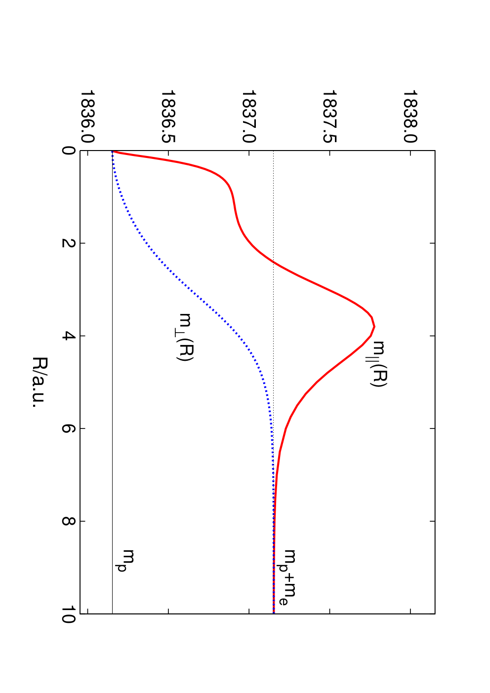
In a molecule, the moving nuclei are ’coated’ with electrons and the amount of additional mass carried by the nuclei changes with $R$ . For a homonuclear molecule in a purely vibrational state, the effective mass of the nucleus at given $R$ , $m_{\|}(R)$ , is just twice the reduced mass $\mu_{\|}(R)$ defined in Eq. (53). Analogously, for a rigid rotating molecule, the effective nuclear mass $m_{\perp}(R)$ is related to $\mu_{\perp}(R)$ of Eq. (54). Thus, their $R$ -dependence can be determined explicitly from the potentials $\mathcal{W}_{\|}(R)$ and $\mathcal{W}_{\perp}(R)$ , respectively. Fig. 2 illustrates the changes in the two effective nuclear masses with the internuclear distance in H₂. The functions $m_{\|}(R)$ and $m_{\perp}(R)$ join smoothly the proton mass at the united atom limit with the hydrogen atomic mass ( $m_{\mathrm{p}}+m_{\mathrm{e}}$ ) at the separated atoms limit. Interestingly, for $R\geq 2.41$ a.u., the effective mass $m_{\|}(R)$ is greater than the sum of proton and electron masses, reaching $m_{\mathrm{p}}+1.6\,m_{\mathrm{e}}$ at the maximum located near $R=3.8$ a.u.

The radial equation (73) has been solved for all bound states with three versions of the potential $\mathcal{Y}(R)$ :

\begin{array}[]{ll}\mathcal{Y}(R)={\cal E}_{\rm el}(R),&{\rm BO}\\ \mathcal{Y}(R)={\cal E}_{\rm el}(R)+{\cal E}_{\rm a}(R),&{\rm adiabatic}\\ \mathcal{Y}(R)={\cal E}_{\rm el}(R)+{\cal E}_{\rm a}(R)+\delta{\cal E}_{\rm na}(R),&{\rm nonadiabatic}\end{array}

yielding three sets of dissociation energies. The corresponding dissociation thresholds were $-1$ hartree in the BO approximation, $-1+m_{\mathrm{e}}/m_{\mathrm{p}}$ hartree in adiabatic approximation, and $-1+m_{\mathrm{e}}/m_{\mathrm{p}}-\left(m_{\mathrm{e}}/m_{\mathrm{p}}\right)^{2}$ hartree in the nonadiabatic level of theory. The results are listed in Table 2, where for each pair of quantum numbers $v$ and $J$ three entries are given (in cm^-1): the BO dissociation energy, the adiabatic correction, and the nonadiabatic correction to the dissociation energy. Thus, the total nonrelativistic dissociation energy can be obtained by summing up all three entries. The only exception is the state with $v=14$ and $J=4$ , for which a nonadiabatic level lying just beneath the dissociation threshold has been predicted although neither BO nor adiabatic bound states exist. The entry given for this state is the energy separation from the nonadiabatic dissociation threshold.

Our nonadiabatic corrections agree very well with those computed by Wolniewicz [15] for rovibrational states of $J\leq 10$ . For all rotational states of the lowest vibrational level the difference is merely 0.0002 cm^-1 or less. In all the cases the difference is smaller than $0.1\%$ , which corresponds to the magnitude of the neglected higher order terms of relative order $\mathcal{O}(1/\mu_{\rm n})$ . This is the first confirmation of the Wolniewicz’s results [15] for $J>0$ rovibrational states and, simultaneously, a numerical validation of the nonadiabatic perturbation theory presented in this work. Let us note, that the nonadiabatic corrections to the dissociation energy from Table 2 differ in sign from the corrections to the adiabatic energy of [15] and their absolute values differ by the constant $1/m_{\mathrm{p}}^{2}=0.06509787$ cm^-1 corresponding to the asymptotic value of the nonadiabatic potential $\delta\mathcal{E}_{\mathrm{na}}(R)$ , discussed in Subsec. III.4.

VI Summary

We have presented the nonadiabatic perturbation theory applicable to any molecule in an arbitrary rovibrational state. The leading nonadiabatic corrections for the diatomic molecule are expressed in terms of three $R$ -dependent functions depicted in Fig. 1: the nuclear reduced mass in Eq. (53), the moment of inertia in Eq. (54), and the correction Eq. (49) to the adiabatic potential, which enter the radial Schrödinger equation for nuclei Eq. (51). This equation can be solved for an arbitrary molecular states by standard numerical methods [21]. Although representation of the nonadiabatic correction by pseudopotentials has been studied previously (see [9, 11, 12] and references therein), we have rigorously derived new expressions for ${\cal W}_{\|}$ , ${\cal W}_{\perp}$ , and $\delta{\cal E}_{\rm na}$ functions of the internuclear distance, which give nonadiabatic corrections with $O(m_{\rm e}/\mu_{\rm n})$ accuracy. Moreover, we have performed explicit numerical calculations for the simplest example of H₂ molecule in order to verify the obtained perturbative formulae. All the electronic matrix elements with differentiation of the wave function over the internuclear distance were rewritten in a convenient form involving differentiation of the Coulomb potential. Such an approach enables achieving much higher numerical precision even for the well known adiabatic correction. The final accuracy of all three nonadiabatic functions is limited only by the neglected higher order terms, namely $\mathcal{O}(m_{\rm e}/\mu_{\rm n})$ relative to the leading order, and results for rovibrational levels agree within this uncertainty with former results of Wolniewicz [15]. Having accurate nonrelativistic energies one can include relativistic and QED corrections, which become significant for the states close to the dissociation threshold. Relativistic corrections for the electronic ground state of H₂ are known accurately for a wide range of internuclear distances [23]. Their large $R$ asymptotics, including QED corrections, is presently investigated by the Jeziorski group [24]. Combining all the knowledge together would enable achieving at least an order of magnitude increase in the precision of theoretical prediction for all molecular states of H₂.

Analogous calculations can be performed for D₂ and HD molecules. It is worth noting, that in the former case there is no need to recompute the pseudopotentials and only a proper rescaling due to different reduced masses is required. The calculations on the latter system, due to difference in mass of the proton and deuteron, would involve additional correction to $\delta{\cal E}_{\rm na}$ coming from the last term of Eq. (5). While this perturbative approach can be further extended to larger diatomic molecules, it would be more challenging to investigate three-atomic molecules such as H ${}_{3}^{+}$ —a system of great astrophysical interest. We expect no principal difficulties in such calculations except for much more increased demands in computer resources needed to perform optimization of pertinent wave functions.

Acknowledgments

We are indebted to L. Wolniewicz for valuable comments. Part of the computations has been performed in Poznań Supercomputing and Networking Center.

References

[1] W. Kołos and L. Wolniewicz, Rev. Mod. Phys. 35, 473 (1963).
[2] S. Bubin and L. Adamowicz, J. Chem. Phys. 118, 3079 (2003).
[3] M. Cafiero and L. Adamowicz, J. Chem. Phys. 122, 184305 (2005).
[4] S. Bubin, L. Adamowicz, and M. Molski, J. Chem. Phys. 123, 134310 (2005).
[5] M. Stanke, D. Kȩdziera, S. Bubin, M. Molski, and L. Adamowicz, Phys. Rev. A 76, 052506 (2008).
[6] M. Born and J. R. Oppenheimer, Ann. Phys. 84, 457 (1927).
[7] M. Born and K. Huang, Dynamical Theory of Crystal Lattices, Oxford University Press (1955) Appendix 8.
[8] R. M. Herman and A. Asgharian, J. Mol. Spectr. 19, 305 (1966).
[9] P. R. Bunker and R. E. Moss, Molec. Phys. 33, 417 (1977), ibid 33, 425 (1977).
[10] R. M. Herman and J. F. Ogilvie. Adv. Chem. Phys. 103, 187 (1998).
[11] W. Kutzelnigg, Mol. Phys. 105, 2627 (2007).
[12] R. Jaquet and W. Kutzelnigg, Chem. Phys. 346, 69 (2008).
[13] D.W. Schwenke, J. Phys. Chem. A 105, 2352 (2001).
[14] P. R. Bunker and R. E. Moss, J. Mol. Spectrosc. 80, 217 (1980).
[15] L. Wolniewicz, J. Chem. Phys. 103, 1792 (1995).
[16] K. Pachucki and J. Komasa, J. Chem. Phys. 129, 034102 (2008).
[17] M. Stanke, D. Kȩdziera, S. Bubin, M. Molski, and L. Adamowicz, J. Chem. Phys. 128, 114313 (2008).
[18] G. Łach, PhD thesis, University of Warsaw (2008).
[19] W. Cencek, private communication.
[20] J. S. Sims and S. A. Hagstrom, J. Chem. Phys. 124, 094101 (2006).
[21] W. Johnson, Atomic Structure Theory (Springer, 2007).
[22] P. J. Mohr and B. N. Taylor, Rev. Mod. Phys. 77, 1 (2005).
[23] L. Wolniewicz, J. Chem. Phys. 99, 1851 (1993).
[24] K. Piszczatowski, G. Łach, and B. Jeziorski, Phys. Rev. A 77, 062514 (2008).

Table 2: The dissociation energy of the rovibrational states of H₂ (in cm^-1). For each pair of vibrational (

v

) and rotational (

J

) quantum numbers, three entries are given: the BO dissociation energy, the adiabatic correction, and the nonadiabatic correction. The sum of the three numbers gives the total nonrelativistic dissociation energy of the (

v

J

) state.

$v\backslash J$	$0$	$1$	$2$	$3$	$4$	$5$	$6$	$7$
0	$36112.5927$	$35994.0372$	$35758.0143$	$35406.6660$	$34943.1216$	$34371.4040$	$33696.3152$	$32923.3094$
0	$5.7711$	$5.8348$	$5.9611$	$6.1481$	$6.3931$	$6.6924$	$7.0418$	$7.4367$
0	$0.4339$	$0.4406$	$0.4539$	$0.4739$	$0.5005$	$0.5338$	$0.5736$	$0.6200$
1	$31949.1892$	$31836.5534$	$31612.3337$	$31278.6001$	$30838.3755$	$30295.5437$	$29654.7385$	$28921.2187$
1	$7.1740$	$7.2311$	$7.3443$	$7.5119$	$7.7310$	$7.9983$	$8.3096$	$8.6605$
1	$1.2704$	$1.2761$	$1.2874$	$1.3044$	$1.3271$	$1.3555$	$1.3896$	$1.4294$
2	$28021.4345$	$27914.5889$	$27701.9154$	$27385.4159$	$26968.0130$	$26453.4605$	$25846.2343$	$25151.4125$
2	$8.3336$	$8.3840$	$8.4839$	$8.6314$	$8.8240$	$9.0583$	$9.3304$	$9.6358$
2	$2.0271$	$2.0318$	$2.0414$	$2.0557$	$2.0749$	$2.0989$	$2.1279$	$2.1618$
3	$24324.4498$	$24223.3066$	$24022.0055$	$23722.4851$	$23327.5744$	$22840.9061$	$22266.8106$	$21610.1998$
3	$9.2420$	$9.2855$	$9.3714$	$9.4982$	$9.6632$	$9.8633$	$10.0945$	$10.3525$
3	$2.7088$	$2.7127$	$2.7206$	$2.7326$	$2.7485$	$2.7686$	$2.7929$	$2.8214$
4	$20855.2072$	$20759.7245$	$20569.7150$	$20287.0583$	$19914.4976$	$19455.5548$	$18914.4286$	$18295.8815$
4	$9.8890$	$9.9251$	$9.9966$	$10.1017$	$10.2378$	$10.4019$	$10.5902$	$10.7985$
4	$3.3187$	$3.3219$	$3.3283$	$3.3379$	$3.3508$	$3.3670$	$3.3868$	$3.4100$
5	$17612.7145$	$17522.9036$	$17344.2107$	$17078.4626$	$16728.3253$	$16297.2225$	$15789.2368$	$15209.0018$
5	$10.2629$	$10.2915$	$10.3476$	$10.4298$	$10.5356$	$10.6618$	$10.8049$	$10.9606$
5	$3.8576$	$3.8599$	$3.8647$	$3.8719$	$3.8816$	$3.8938$	$3.9087$	$3.9262$
6	$14598.2891$	$14514.2237$	$14346.9982$	$14098.3935$	$13771.0098$	$13368.1874$	$12893.9129$	$12352.7160$
6	$10.3525$	$10.3729$	$10.4130$	$10.4712$	$10.5449$	$10.6313$	$10.7268$	$10.8271$
6	$4.3218$	$4.3232$	$4.3262$	$4.3306$	$4.3365$	$4.3440$	$4.3531$	$4.3639$
7	$11815.9479$	$11737.7779$	$11582.3242$	$11351.3310$	$11047.3466$	$10673.6480$	$10234.1517$	$9733.3170$
7	$10.1486$	$10.1606$	$10.1839$	$10.2169$	$10.2573$	$10.3020$	$10.3476$	$10.3901$
7	$4.7029$	$4.7031$	$4.7037$	$4.7044$	$4.7055$	$4.7067$	$4.7081$	$4.7095$
8	$9272.9561$	$9200.9278$	$9057.7445$	$8845.1263$	$8565.5890$	$8222.3732$	$7819.3619$	$7360.9906$
8	$9.6483$	$9.6517$	$9.6577$	$9.6648$	$9.6707$	$9.6726$	$9.6670$	$9.6500$
8	$4.9838$	$4.9824$	$4.9796$	$4.9752$	$4.9692$	$4.9614$	$4.9516$	$4.9393$
9	$6980.5984$	$6915.0837$	$6784.9238$	$6591.8323$	$6338.3203$	$6027.6323$	$5663.6708$	$5250.9187$
9	$8.8590$	$8.8537$	$8.8422$	$8.8232$	$8.7945$	$8.7533$	$8.6963$	$8.6196$
9	$5.1364$	$5.1325$	$5.1246$	$5.1124$	$5.0958$	$5.0743$	$5.0472$	$5.0138$
10	$4955.2699$	$4896.8118$	$4780.7739$	$4608.8912$	$4383.7137$	$4108.5514$	$3787.4126$	$3424.9438$
10	$7.8021$	$7.7882$	$7.7597$	$7.7151$	$7.6525$	$7.5691$	$7.4616$	$7.3260$
10	$5.1160$	$5.1082$	$5.0925$	$5.0684$	$5.0354$	$4.9926$	$4.9386$	$4.8720$
11	$3220.0418$	$3169.4253$	$3069.1017$	$2920.8723$	$2727.3991$	$2492.1652$	$2219.4373$	$1914.2414$
11	$6.5140$	$6.4918$	$6.4469$	$6.3777$	$6.2821$	$6.1573$	$5.9996$	$5.8045$
11	$4.8566$	$4.8429$	$4.8151$	$4.7725$	$4.7140$	$4.6379$	$4.5418$	$4.4224$
12	$1806.9489$	$1765.3260$	$1683.0605$	$1562.1049$	$1405.3733$	$1216.7368$	$1001.0464$	$764.2101$
12	$5.0372$	$5.0068$	$4.9451$	$4.8505$	$4.7203$	$4.5506$	$4.3360$	$4.0685$
12	$4.2657$	$4.2429$	$4.1965$	$4.1254$	$4.0271$	$3.8984$	$3.7345$	$3.5281$
13	$760.3903$	$729.5279$	$668.9437$	$580.9383$	$469.0254$	$338.0600$	$194.5461$	$47.4825$
13	$3.3933$	$3.3526$	$3.2697$	$3.1417$	$2.9631$	$2.7253$	$2.4123$	$1.9886$
13	$3.2221$	$3.1850$	$3.1095$	$2.9927$	$2.8294$	$2.6113$	$2.3232$	$1.9317$
14	$141.7951$	$124.7523$	$92.3077$	$48.0033$
14	$1.5343$	$1.4739$	$1.3479$	$1.1416$
14	$1.5847$	$1.5226$	$1.3933$	$1.1825$	$0.0887^{\dagger}$

^† This state appears as a resonance in BO and adiabatic approximations. The entry is a dissociation energy of this nonadiabatic level.

Table 2: continued

$v\backslash J$	$8$	$9$	$10$	$11$	$12$	$13$	$14$	$15$
0	$32058.3583$	$31107.8190$	$30078.3065$	$28976.5781$	$27809.4302$	$26583.6105$	$25305.7462$	$23982.2860$
0	$7.8718$	$8.3418$	$8.8411$	$9.3642$	$9.9055$	$10.4596$	$11.0212$	$11.5852$
0	$0.6728$	$0.7322$	$0.7981$	$0.8704$	$0.9491$	$1.0343$	$1.1260$	$1.2240$
1	$28100.7394$	$27199.4234$	$26223.6397$	$25179.8929$	$24074.7260$	$22914.6378$	$21706.0160$	$20455.0847$
1	$9.0458$	$9.4605$	$9.8991$	$10.3562$	$10.8264$	$11.3045$	$11.7850$	$12.2629$
1	$1.4749$	$1.5263$	$1.5834$	$1.6464$	$1.7154$	$1.7903$	$1.8713$	$1.9584$
2	$24374.5496$	$23521.5539$	$22598.5709$	$21611.8782$	$20567.7938$	$19472.5994$	$18332.4783$	$17153.4682$
2	$9.9697$	$10.3271$	$10.7026$	$11.0910$	$11.4869$	$11.8851$	$12.2802$	$12.6671$
2	$2.2008$	$2.2449$	$2.2942$	$2.3488$	$2.4089$	$2.4744$	$2.5456$	$2.6225$
3	$20876.4463$	$20071.2651$	$19200.6029$	$18270.5391$	$17287.1990$	$16256.6838$	$15185.0135$	$14078.0862$
3	$10.6327$	$10.9300$	$11.2393$	$11.5554$	$11.8729$	$12.1865$	$12.4908$	$12.7804$
3	$2.8543$	$2.8917$	$2.9337$	$2.9804$	$3.0320$	$3.0885$	$3.1500$	$3.2167$
4	$17605.1247$	$16847.7045$	$16029.3982$	$15156.1198$	$14233.8415$	$13268.5282$	$12266.0890$	$11232.3425$
4	$11.0221$	$11.2561$	$11.4954$	$11.7348$	$11.9690$	$12.1923$	$12.3995$	$12.5849$
4	$3.4370$	$3.4677$	$3.5023$	$3.5409$	$3.5836$	$3.6304$	$3.6814$	$3.7365$
5	$14561.5917$	$13852.4141$	$13087.1119$	$12271.4764$	$11411.3755$	$10512.6972$	$9581.3093$	$8623.0355$
5	$11.1244$	$11.2915$	$11.4566$	$11.6146$	$11.7601$	$11.8873$	$11.9906$	$12.0642$
5	$3.9466$	$3.9699$	$3.9962$	$4.0254$	$4.0576$	$4.0926$	$4.1304$	$4.1704$
6	$11749.5653$	$11089.7678$	$10378.8781$	$9622.6208$	$8826.8275$	$7997.3920$	$7140.2429$	$6261.3368$
6	$10.9279$	$11.0242$	$11.1110$	$11.1829$	$11.2344$	$11.2597$	$11.2528$	$11.2071$
6	$4.3763$	$4.3903$	$4.4058$	$4.4226$	$4.4406$	$4.4592$	$4.4779$	$4.4957$
7	$9176.0486$	$8567.6048$	$7913.5170$	$7219.5226$	$6491.5173$	$5735.5270$	$4957.7045$	$4164.3543$
7	$10.4250$	$10.4474$	$10.4524$	$10.4343$	$10.3876$	$10.3060$	$10.1831$	$10.0114$
7	$4.7108$	$4.7118$	$4.7119$	$4.7108$	$4.7076$	$4.7012$	$4.6902$	$4.6724$
8	$6852.1602$	$6298.1569$	$5704.5851$	$5077.3199$	$4422.4828$	$3746.4465$	$3055.8806$	$2357.8507$
8	$9.6172$	$9.5638$	$9.4847$	$9.3741$	$9.2260$	$9.0337$	$8.7892$	$8.4833$
8	$4.9241$	$4.9053$	$4.8820$	$4.8528$	$4.8160$	$4.7692$	$4.7092$	$4.6313$
9	$4794.3657$	$4299.4465$	$3771.9991$	$3218.2507$	$2644.8437$	$2058.9184$	$1468.2878$	$881.7751$
9	$8.5188$	$8.3891$	$8.2250$	$8.0203$	$7.7678$	$7.4587$	$7.0814$	$6.6193$
9	$4.9730$	$4.9232$	$4.8624$	$4.7880$	$4.6962$	$4.5819$	$4.4375$	$4.2515$
10	$3026.3806$	$2597.5217$	$2144.7391$	$1675.0460$	$1196.2612$	$717.3517$	$249.1650$
10	$7.1577$	$6.9514$	$6.7003$	$6.3963$	$6.0280$	$5.5786$	$5.0193$
10	$4.7905$	$4.6909$	$4.5694$	$4.4200$	$4.2343$	$3.9995$	$3.6930$
11	$1582.3694$	$1230.4417$	$866.0734$	$498.2452$	$138.1669$
11	$5.5658$	$5.2756$	$4.9227$	$4.4892$	$3.9416$
11	$4.2752$	$4.0939$	$3.8689$	$3.5852$	$3.2148$
12	$513.3908$	$257.4738$	$8.3253$
12	$3.7358$	$3.3166$	$2.7633$
12	$3.2682$	$2.9354$	$2.4878$

Table 2: continued

$v\backslash J$	$16$	$17$	$18$	$19$	$20$	$21$	$22$	$23$
0	$22619.4577$	$21223.2371$	$19799.3296$	$18353.1603$	$16889.8728$	$15414.3355$	$13931.1527$	$12444.6818$
0	$12.1465$	$12.7005$	$13.2425$	$13.7681$	$14.2729$	$14.7525$	$15.2029$	$15.6196$
0	$1.3286$	$1.4396$	$1.5572$	$1.6814$	$1.8122$	$1.9497$	$2.0939$	$2.2451$
1	$19167.8656$	$17850.1517$	$16507.4922$	$15145.1868$	$13768.2885$	$12381.6135$	$10989.7585$	$9597.1235$
1	$12.7332$	$13.1911$	$13.6317$	$14.0502$	$14.4420$	$14.8023$	$15.1262$	$15.4086$
1	$2.0516$	$2.1512$	$2.2570$	$2.3693$	$2.4881$	$2.6134$	$2.7453$	$2.8838$
2	$15941.4274$	$14702.0131$	$13440.6714$	$12162.6372$	$10872.9422$	$9576.4337$	$8277.7999$	$6981.6067$
2	$13.0406$	$13.3957$	$13.7272$	$14.0300$	$14.2988$	$14.5281$	$14.7122$	$14.8446$
2	$2.7052$	$2.7938$	$2.8884$	$2.9890$	$3.0955$	$3.2080$	$3.3263$	$3.4502$
3	$12941.6497$	$11781.2863$	$10602.4104$	$9410.2757$	$8209.9952$	$7006.5729$	$5804.9493$	$4610.0657$
3	$13.0501$	$13.2944$	$13.5077$	$13.6843$	$13.8181$	$13.9026$	$13.9307$	$13.8939$
3	$3.2886$	$3.3657$	$3.4479$	$3.5352$	$3.6272$	$3.7237$	$3.8240$	$3.9274$
4	$10172.9970$	$9093.6453$	$7999.7724$	$6896.7794$	$5790.0229$	$4684.8764$	$3586.8202$	$2501.5762$
4	$12.7427$	$12.8672$	$12.9520$	$12.9905$	$12.9756$	$12.8991$	$12.7513$	$12.5207$
4	$3.7957$	$3.8587$	$3.9253$	$3.9948$	$4.0665$	$4.1392$	$4.2113$	$4.2803$
5	$7643.6478$	$6648.8775$	$5644.4446$	$4636.1112$	$3629.7676$	$2631.5640$	$1648.1214$	$686.8842$
5	$12.1016$	$12.0965$	$12.0417$	$11.9291$	$11.7496$	$11.4918$	$11.1414$	$10.6779$
5	$4.2124$	$4.2556$	$4.2990$	$4.3412$	$4.3801$	$4.4126$	$4.4344$	$4.4383$
6	$5366.6735$	$4462.3376$	$3554.5745$	$2649.9163$	$1755.3887$	$878.8631$	$29.7112$
6	$11.1158$	$10.9712$	$10.7645$	$10.4851$	$10.1192$	$9.6476$	$9.0402$
6	$4.5115$	$4.5235$	$4.5291$	$4.5249$	$4.5055$	$4.4629$	$4.3836$
7	$3361.9951$	$2557.4749$	$1758.1694$	$972.3301$	$209.7400$
7	$9.7827$	$9.4869$	$9.1113$	$8.6376$	$8.0373$
7	$4.6449$	$4.6038$	$4.5430$	$4.4532$	$4.3193$
8	$1660.0067$	$970.9237$	$300.7647$
8	$8.1037$	$7.6332$	$7.0443$
8	$4.5286$	$4.3911$	$4.2015$
9	$309.8952$
9	$6.0447$
9	$4.0047$

Table 2: continued

$v\backslash J$	$24$	$25$	$26$	$27$	$28$	$29$	$30$	$31$
0	$10959.0542$	$9478.2014$	$8005.8846$	$6545.7303$	$5101.2727$	$3676.0048$	$2273.4444$	$897.2218$
0	$15.9981$	$16.3340$	$16.6221$	$16.8572$	$17.0329$	$17.1423$	$17.1769$	$17.1261$
0	$2.4031$	$2.5682$	$2.7404$	$2.9199$	$3.1066$	$3.3006$	$3.5019$	$3.7105$
1	$8207.9415$	$6826.3161$	$5456.2676$	$4101.7929$	$2766.9437$	$1455.9363$	$173.3131$
1	$15.6440$	$15.8264$	$15.9492$	$16.0045$	$15.9831$	$15.8734$	$15.6600$
1	$3.0290$	$3.1807$	$3.3389$	$3.5032$	$3.6734$	$3.8488$	$4.0283$
2	$5692.3452$	$4414.4956$	$3152.6140$	$1911.4560$	$696.1630$
2	$14.9184$	$14.9254$	$14.8559$	$14.6980$	$14.4356$
2	$3.5795$	$3.7135$	$3.8516$	$3.9923$	$4.1340$
3	$3426.9550$	$2260.8735$	$1117.5022$
3	$13.7827$	$13.5850$	$13.2850$
3	$4.0327$	$4.1379$	$4.2403$
4	$1435.3165$	$395.0112$
4	$12.1920$	$11.7435$
4	$4.3427$	$4.3926$

Nonadiabatic corrections to rovibrational levels of H2

Abstract

pacs

I Introduction

II The adiabatic approximation

III Perturbative formalism

III.1 Second-order nonadiabatic corrections

III.2 Third-order nonadiabatic correction

III.3 Nuclear equation with effective potentials

III.4 Asymptotics of the effective masses

III.5 Evaluation of the wave function derivatives

IV Numerical calculations

V Results and discussion

VI Summary

Acknowledgments

References

Nonadiabatic corrections to rovibrational levels of H₂