Parameter degeneracies and (un)predictability of gravitational microlensing events
Abstract
Some of the difficulties in determining the underlying physical properties that are relevant for observed anomalies in microlensing light curves, such as the mass and separation of extra-solar planets orbiting the lens star, or the relative source-lens parallax, are already anchored in factors that limit the amount of information available from ordinary microlensing events and in the way these are being parametrized. Moreover, a real-time detection of deviations from an ordinary light curve while these are still in progress can only be done against a known model of the latter, and such is also required for properly prioritizing ongoing events for monitoring in order to maximize scientific returns. Despite the fact that ordinary microlensing light curves are described by an analytic function that only involves a handful of parameters, modelling these is far less trivial than one might be tempted to think. A well-known degeneracy for small impacts, and another one for the initial rise of an event, makes an interprediction of different phases impossible, while in order to determine a complete set of model parameters, the fundamental characteristics of all these phases need to be properly assessed. While it is found that the wing of the light curve provides valuable information about the time-scale that absorbs the physical properties, the peak flux of the event can be meaningfully predicted only after about a third of the total magnification has been reached. Parametrizations based on observable features not only ease modelling by bringing the covariance matrix close to diagonal form, but also allow good predictions of the measured flux without the need to determine all parameters accurately. Campaigns intending to infer planet populations from observed microlensing events need to invest some fraction of the available time into acquiring data that allows to properly determine the magnification function.
Keywords:
gravitational lensing – planetary systems.1 Introduction
An efficient detection of planets by means of gravitational microlensing requires sufficiently accurate predictions of the underlying ordinary light curve against which the planetary deviations need to be identified (Dominik et al., 2007; Dominik et al., 2008). An optimal monitoring strategy in order to maximize the scientific return moreover profits strongly from the proper determination of a full set of model parameters as early as possible, and the latter becomes a requirement for finally assessing the planet detection efficiency and drawing conclusions about the planet population.
It is known that early-stage event prediction suffers from degeneracies (Albrow, 2004), in particular the peak flux is hard to assess, while the event time-scale , required to relate the observations to the underlying physical properties, can remain strongly uncertain even after the event has been observed over its full course, but not covered well enough (Woźniak & Paczyński, 1997). The lack of determinacy of is particularly apparent for strongly-blended events, which in fact comprise the full sample for observations towards neighbouring galaxies such as M31 (Baillon et al., 1993, e.g.).
Understanding of ordinary light curves (comprising single point-like source and lens stars), their optimal parametrization, and the apparent degeneracies and ambiguities, is also crucial and useful for modelling events that involve anomalies, and drawing conclusions about e.g. stellar binaries, stellar masses derived from parallax measurements, and planets. Sparse event coverage in critical regions is even prone to lead to ordinary events allowing for multiple minima of the (least-squares) hypersurface, this fact being further complicated by the presence of potential outliers in the data and the application of robust-estimation techniques to deal with these (Dominik et al., 2007, e.g.).
In this paper, different phases of ordinary microlensing events along with their characteristics are identified, and it is shown how feature-oriented parametrizations can be used to quantify the behaviour while avoiding parameter correlations. Moreover, some fundamental requirements for a monitoring strategy that allows to meet the goal of determining either the observed flux or the corresponding magnification are discussed. The basis for this is formed by approximate relations between the magnification and the angular separation between lens and source that make the light curve independent of the impact parameter. Together with some arising degeneracies, these have already been identified by Woźniak & Paczyński (1997), but here some new light is shed on the implications and the focus is on different aspects that are emergent right now, which leads to arriving at some new and different conclusions.
While Sect. 2 reviews the general properties of ordinary microlensing events and the canonical parametrization, and Sect. 3 presents the advantages of an alternative parametrization that is oriented towards the observable characteristic features, Sect. 4 discusses the predictability of ordinary microlensing events or the lack of it. A summary and final conclusions are provided in Sect. 5.
2 The canonical treatment of ordinary events
A microlensing event results if two stars happen to be closely aligned as seen from Earth, where this alignment is quantified by the unique characteristic scale of gravitational microlensing, namely the angular Einstein radius (Einstein, 1936)
| (1) |
where denotes the mass of the foreground lens star, is the universal gravitational constant, is the vacuum speed of light, and
| (2) |
stands for the relative source-lens parallax, with and being the distance from Earth to the foreground (lens) star and the observed background source star, respectively. With denoting the angular separation between lens and source star, gravitational bending of light by the lens star yields an observable magnification of the source star as an analytic function of , which reads
| (3) |
Stellar kinematics implies a non-vanishing relative proper motion between lens and source star, so that is a function of time and the magnification describes a characteristic light curve. While in the earlier history of gravitational microlensing several different event time-scales have been used (Griest, 1991; de Rújula et al., 1991, e.g.), has emerged as a popular convenient choice.
For uniform proper motion, i.e. constant , the dimensionless separation can be expressed by means of three quantities that form the parameter vector , so that
| (4) |
where is the smallest angular separation, encountered at epoch , while the source moves by an angular Einstein radius relative to the lens within the time-scale (Paczyński, 1986). Whereas and only define the position of the trajectory of the source relative to the lens, and therefore do not carry any information about the relevant physical properties that determine the magnification, which are the relative parallax , the relative proper motion , and the lens mass , all these are convolved into the event time-scale . It is in fact its relation to the physical event properties that makes the parameter a preferred choice amongst possible time-scales. As illustrated in Fig. 1, ordinary light curves: (1) are symmetric with respect to a peak at epoch , (2) reach a peak flux there, (3) approach a baseline flux for times far away from the peak, and (4) show characteristic inflection points. However, the parameter is the only one that directly relates to the characteristic features of the light curve, while all the others are not a proper reflection. This is not at all favourable for modelling, and instead being able to essentially read off the model parameters from the collected data would ease life a lot.
The phenomenon of gravitational microlensing leads to a characteristic magnification as a function of time and the model parameters that describe the lens-observer-source geometry, the lens properties, and the source brightness profile. The observed flux for a given site and passband — denoted by the multi-index —, however, furthermore is a linear function of the intrinsic flux of the observed source star , which is magnified, and a background flux , where (Albrow et al., 2000, e.g.)
| (5) |
This allows us to isolate these two parameters from the remaining parameter space, so that
| (6) |
and for every value of , minimizing
| (7) |
thereby obtaining a maximum-likelihood estimate of the parameter vector , means that the best-fitting source and background fluxes can be expressed in closed analytical form (Rattenbury, 2003)
| (8) |
while the non-linear minimization process can be restricted to
| (9) |
expressed by means of the magnification rather than the flux, where
| (10) |
and
| (11) |

3 Parameters that match observational features
It is well known that avoiding parameter degeneracies and strong correlations eases the modelling process. Moreover, a careful study of these provides valuable insight into the structure of parameter space, which can be used as a guide for developing observing strategies and explicitly shows their limitations. For ordinary microlensing light curves, it turns out that the observed flux can be rewritten by means of a different parametrization that better matches the observational features, which are key to diagonalizing the covariance matrix.
With the baseline flux and the peak flux given by
| (12) |
the maximal flux difference reads
| (13) |
Not only in and , but also in and , the observed flux is a linear function, namely
| (14) |
so that these parameters can be separated by a linear fit as well. One can then define a half-maximum time , so that at time , half of the flux offset is encountered, i.e.
| (15) |
This means that the epochs correspond to a magnification
| (16) |
With and by means of Eq. (4), one finds
| (17) |
which leads to
| (18) |
If one now plots the offset flux in units of the difference between peak and baseline, and scales with rather than , as illustrated in Fig. 2, one finds that light curves with different nearly coincide around their peaks. In contrast, it is the wing region of the event that is best-suited to provide information about the impact parameter , and thereby of the event time-scale , related to the underlying physical properties.11 1 The subsequent section shows that the asymptotic degeneracy for large does not extend into this region. In principle, is determined by the slope of the light curve at , but the narrow range22 2 The absolute value of the slope ranges between 0.375 (for ) and (for ). strongly limits the feasibility of such an approach in practice.

It is also instructive to explore the limits of small and large separations more closely. Both for and , the observed relative flux offset becomes independent of , while becomes proportional to , however with different proportionality factors for the two extreme cases. As summarized in Table 1, this is due to the fact that the magnification can reasonably well be approximated by a more simple expression, namely approaching for , and for . For , one retrieves the known results that apply to microlensing of unresolved sources where , being an inevitability for observations towards M31 or other nearby other galaxies (Baillon et al., 1993; Woźniak & Paczyński, 1997). Looking at Fig. 2 again, one sees that all light curves range between the two extreme cases
| (19) |
The wings of the light curves converge towards the expression for , where for smaller , the transition from the to the asymptotic occurs at larger .
4 Different event phases and the lack of predictability
One might think that 3 parameters (like , , and ) can be obtained straightforwardly by means of regression from as few as 4 data points, but such an attempt fails if the observable does not significantly change with a variation of the considered parameter. So far, it has been assumed that the light curve has been sampled over its full course, so that a full set of characteristics can be determined from which model parameters can be derived. However, the light curve develops in time, so that some characteristics are not accessible at early stages. While the baseline flux is being observed much before any rise in brightness occurs, the peak flux or the flux shift , respectively, remain unknown, as we shall see more explicitly in the following.
Reviewing the asymptotics for and from a different perspective already shows us that there is no interpredictability between the peak and wing regions of the observed light curve, and in particular, early observations give poor estimates of the peak magnification, as well as on the time-scale . In particular, maximum-likehihood estimates corresponding to values that minimize , Eq. (9), frequently yield very small , far away from expectations. Therefore, Albrow (2004) has suggested to use a maximum-a-posteriori estimate instead, incorporating the actual distribution of the parameters of the observed events of the microlensing surveys as prior.
Let us look into this with a view on the parameter degeneracies. The earliest stages of an event are characterized by , so that . For the two extreme cases of being far from unity, one finds
| (20) |
where the second case is realized for a substantial time interval if is sufficiently small.
With the blend ratio , the observed flux can be written as
| (21) | |||||
so that
| (22) |
where
| (23) |
are characteristic rise times, absorbing and , with for .
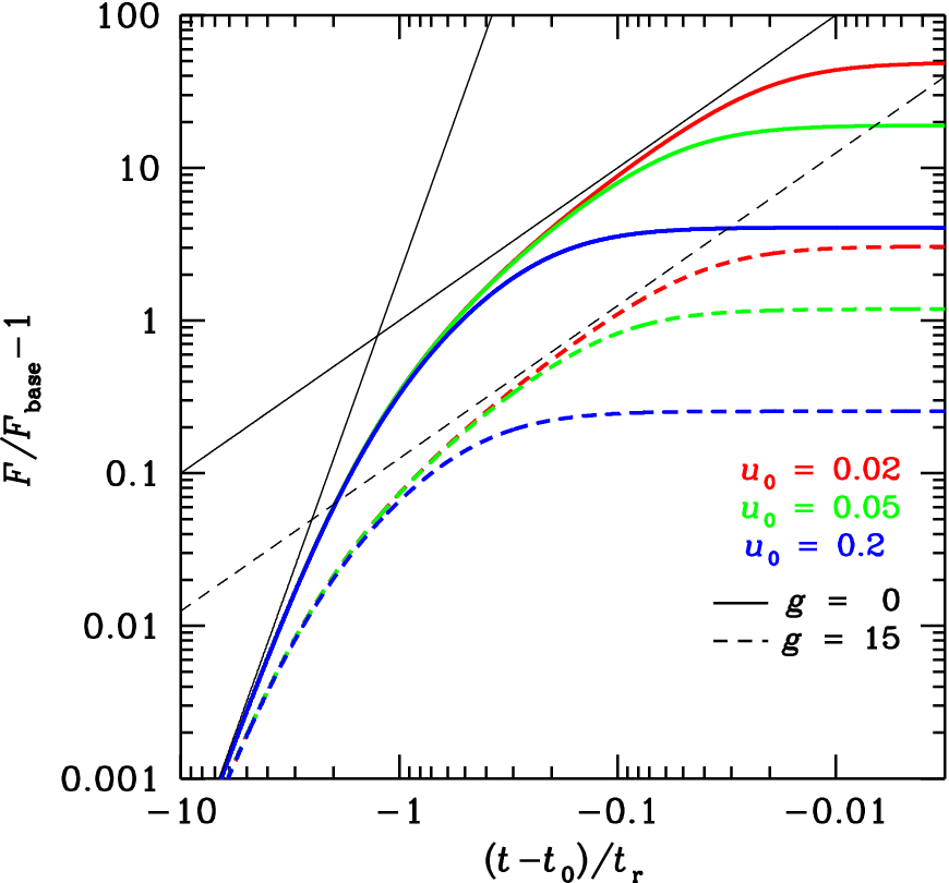
Figure 3 shows as a function of in a double-logarithmic plot, so that the approximate relations of Eq. (22) correspond to straight lines. It illustrates that different behaviour allows to distinguish three phases of a microlensing event, corresponding to the initial rise, a mid-phase, and the peak approach, where a determination of the full model parameter set requires an assessment of the fundamental characteristics of all these phases. With the approximate diverging as , an estimate for based on such an approximation corresponds to . Only a departure from the approximation in the form of an evident turn-off gives evidence for non-vanishing . However, as Fig. 3 illustrates, this happens at rather late stage, and roughly when a third of the peak magnification has been reached. Given that for , differs substantially from the asymptotic behaviour for , the blend ratio can in principle be determined rather early, which then provides the time-scale that is related to the underlying physical properties of the event. In practice this requires sufficiently dense and precise measurements, which are frequently not available for fluxes close to , but the long duration of the rise phase in principle allows for lots of data to be collected. Nevertheless, as soon as both and can be determined from the acquired data, the blend ratio and are known. Again, one sees the power of observations covering the wing of the light curve.

Going the other way round and coming from the peak, the microlensing light curve first follows the decay with , then enters the mid-phase characterized by , and finally follows a decrease described by . Double-logarithmic plots of the relative offset brightening as a function of are shown in Fig. 4, while the relevant magnifications, impact parameters, and time-scales for the selected cases are listed in Table 2. Again, one sees that the light curves for different blend ratio and can be made to match well near the peak, whereas observations in the wing of the light curve on the departure from the asymptotic mid-phase behaviour () or on the transition into the baseline-approach phase () are useful to determine . The rather long duration of these phases favours such an attempts by not requiring a high sampling rate for obtaining a larger number of measurements.
| 50 | 50 | 25.5 | 0.0200 | 0.0392 | 29.6 | 29.6 | 29.6 |
| 20 | 20 | 10.5 | 0.0500 | 0.0956 | 12.3 | 12.3 | 12.3 |
| 5 | 5 | 3 | 0.203 | 0.348 | 3.53 | 3.53 | 3.53 |
| 50 | 785 | 393 | 0.00127 | 0.00255 | 453 | 227 | 28.4 |
| 20 | 305 | 153 | 0.00328 | 0.00654 | 177 | 88.4 | 11.1 |
| 5 | 65 | 33 | 0.0154 | 0.0303 | 38.3 | 19.1 | 2.39 |
for , while for .
5 Summary and final conclusions
Despite the fact that the timescale , where denotes the angular Einstein radius, and the relative proper motion between lens and source star, is the crucial one for drawing conclusions about the underlying physical properties that led to a microlensing event, it is not a good choice for describing the observable characteristic features, and thereby not a useful means of describing or predicting events in progress.
Contrary to common belief, 3 model parameters cannot always properly be extracted from a least-squares fit involving at least 4 data points. In fact, such attempts fail if the respective function to be matched to the observed data does not significantly depend on each of the parameters over the region where data have been acquired. Microlensing light curves usually go through 3 phases from baseline to peak as well as from peak back to baseline: Two rise phases characterized by different rise times and , corresponding to different power laws of the magnification with the angular separation between lens and source, as well as a peak region, characterized by a half-width . None of the individual phases contains characteristic information about the complete set of model parameters, and in order to reveal accurate estimates for all of them, each of them requires appropriate coverage. While the mid-phase gets squeezed for impact angles of the order of the angular Einstein radius or larger, the part of the light curve with becomes indistinguishable from the baseline for strongly-blended events, so that on the approach to baseline, the offset magnification is proportional to rather than , given that still for .
It is well-known that an appropriate estimate of event parameters at early event stages is not feasible, and in particular the peak magnification is regularly overpredicted by a maximum-likelihood estimate corresponding to minimizing the sum of normalized squared deviations . Just for this reason, Albrow (2004) had suggested to use a maximum-a-posteriori estimate instead, with a suitable prior. While this brings the estimate closer to its expectation value, it does not get around the uncertainty. A closer eximation shows that the light curve is compatible with an infinite peak flux until roughly a third of the true offset magnification is reached. Moreover, it is a wing region that is best suited to determine the blend ratio (and with it the time-scale , rather than the immediate vicinity of the peak. The rather long duration of this phase allows to obtain a suitable measurement without the need for very dense sampling.
For an accurate prediction of the observed flux, a proper determination of the full set of model parameters is not required, so that local approximations can provide a reasonable substitute. In sharp contrast, proper knowledge of , which implies knowledge of the blend ratio and the magnification , is a requirement for determining the event detection efficiency to planets (Gaudi et al., 2002) as well as for prioritising ongoing events in order to maximize it (Han, 2007; Snodgrass et al., 2008). Without such information, one neither knows the amplitude, nor the duration, nor the location of potentially arising planetary signals. Therefore, an efficient campaign for inferring the planet population from observed microlensing events needs to invest time into observations that allow to properly determine the event parameters, rather than just trying to detect planets in poorly determined events, where unsuitable assumptions about model parameters may yield to bad choices, or efforts could even turn out to be wasted if the planet detection efficiency cannot be assessed. Building upon the findings presented in this paper, a more detailed study of event (un)predictability taking into account the specific capabilities of observing campaigns could hence provide important clues towards optimizing strategies for detecting planets and determining their population statistics.
References
- Albrow et al. (2000) Albrow M. D., et al., 2000, ApJ, 535, 176
- Albrow (2004) Albrow M. D., 2004, ApJ, 607, 821
- Baillon et al. (1993) Baillon P., Bouquet A., Giraud-Heraud Y., Kaplan J., 1993, A&A, 277, 1
- de Rújula et al. (1991) de Rújula A., Jetzer P., Massó E., 1991, MNRAS, 250, 348
- Dominik et al. (2007) Dominik M., et al., 2007, MNRAS, 380, 792
- Dominik et al. (2008) Dominik M., et al., 2008, AN, 329, 248
- Einstein (1936) Einstein A., 1936, Science, 84, 506
- Gaudi et al. (2002) Gaudi B. S., et al., 2002, ApJ, 566, 463
- Griest (1991) Griest K., 1991, ApJ, 366, 412
- Han (2007) Han C., 2007, ApJ, 661, 1202
- Paczyński (1986) Paczyński B., 1986, ApJ, 304, 1
- Rattenbury (2003) Rattenbury N. J., 2003, PhD thesis, University of Auckland
- Snodgrass et al. (2008) Snodgrass C., Tsapras Y., Street R., Bramich D., Horne K., Dominik M., Allan A., 2008, PoS(GMC8)056
- Woźniak & Paczyński (1997) Woźniak P., Paczyński B., 1997, ApJ, 487, 55