blue red green

Optimal Encoding Schemes for Several Classes of Discrete Degraded Broadcast Channels

Bike Xie, Student Member, IEEE, Thomas Courtade, Student Member, IEEE,
and Richard D. Wesel, Senior Member, IEEE ^†^†thanks: This work was supported by the Defence Advanced Research Project Agency SPAWAR Systems Center, San Diego, California under Grant N66001-02-1-8938.
This work was done when Bike Xie was with the Electrical Engineering Department,University of California, Los Angeles. Bike Xie is currently with Marvell Semiconductor Inc. Thomas Courtade and Richard Wesel are with the Electrical Engineering Department,University of California, Los Angeles, CA 90095 USA. (e-mail: bike@marvell.com; tacourta@ucla.edu; wesel@ee.ucla.edu)

Abstract

Consider a memoryless degraded broadcast channel (DBC) in which the channel output is a single-letter function of the channel input and the channel noise. As examples, for the Gaussian broadcast channel (BC) this single-letter function is regular Euclidian addition and for the binary-symmetric BC this single-letter function is Galois-Field-two addition. This paper identifies several classes of discrete memoryless DBCs for which a relatively simple encoding scheme, which we call natural encoding, achieves capacity. Natural Encoding (NE) combines symbols from independent codebooks (one for each receiver) using the same single-letter function that adds distortion to the channel. The alphabet size of each NE codebook is bounded by that of the channel input.

Inspired by Witsenhausen and Wyner, this paper defines the conditional entropy bound function $F^{*}$ , studies its properties, and applies them to show that NE achieves the boundary of the capacity region for the multi-receiver broadcast Z channel. Then, this paper defines the input-symmetric DBC, introduces permutation encoding for the input-symmetric DBC, and proves its optimality. Because it is a special case of permutation encoding, NE is capacity achieving for the two-receiver group-operation DBC. Combining the broadcast Z channel and group-operation DBC results yields a proof that NE is also optimal for the discrete multiplication DBC. Along the way, the paper also provides explicit parametric expressions for the two-receiver binary-symmetric DBC and broadcast Z channel.

Index Terms:

Degraded broadcast channel, natural encoding, broadcast Z channel, input-symmetric, group-operation degraded broadcast channel, discrete multiplication degraded broadcast channel, Gaussian broadcast channel, binary-symmetric broadcast channel.

I Introduction

I-A Background

Nearly four decades ago, Cover [1], Bergmans [2] and Gallager [3] established the capacity region for degraded broadcast channels (DBC). A common optimal transmission strategy to achieve the boundary of the capacity region for DBCs is the joint encoding scheme presented in [1] [2]. Specifically, the information intended for the receiver with the most degraded channel is encoded to produce a first codeword. Conditioned on that first codeword, a codebook is selected for the receiver with the second most degraded channel, and so forth.

There is at least one independent-encoding scheme (in which the codebook for each user is independent of the messages intended for other users) that can achieve the capacity of any DBC [4]. This scheme essentially embeds all symbols from all the needed codebooks for the less-degraded receiver(s) into a single super-symbol (but perhaps with a large alphabet). Then a single-letter function uses the input symbol from the more-degraded receiver to extract the needed symbol from the super symbol provided by the less-degraded receiver. See Appendix A for a detailed description of this encoding scheme.

Cover [5] introduced an independent-encoding scheme for two-receiver broadcast channels (BCs). When applied to two-receiver DBCs, this scheme independently encodes receivers’ messages, and then combines these resulting codewords by applying a single-letter function. This scheme does not specify what codebooks to use or what single-letter function to use. It is a general independent-encoding approach, which includes the independent-encoding scheme described in Appendix A.

Consider DBCs in which the received signal of each component channel can be modeled as a single-letter function of the channel input and the channel noise. A simple encoding scheme that is optimal for some of those DBCs is an independent-encoding approach in which symbols from independent codebooks, each with the same alphabet as the channel input, are combined using the same single-letter function that adds distortion to the channel. We refer to this encoding scheme as the natural encoding (NE) scheme. As an example, the NE scheme for a two-receiver Gaussian BC has as each transmitted symbol the real addition of two real symbols from independent codebooks. The NE scheme is known to achieve the boundary of the capacity region for several BCs including Gaussian BCs [6], binary-symmetric BCs [2] [7] [8] [9], discrete additive DBCs [10] and two-receiver broadcast Z channels [11] [12].

In proving the optimality of NE schemes for Gaussian BCs and binary-symmetric BCs, Shannon’s entropy power inequality (EPI) [13] and “Mrs. Gerber’s Lemma” [14], respectively, play the same significant role. Shannon’s EPI gives a lower bound on the differential entropy of the sum of independent random variables. In Bergmans’s remarkable paper [6], he applied the EPI to establish a converse showing the optimality of the scheme given by [1] [2] (the NE scheme) for Gaussian BCs. Similarly, “Mrs. Gerber’s Lemma” provides a lower bound on the entropy of a sequence of binary-symmetric channel outputs. Wyner and Ziv obtained “Mrs. Gerber’s Lemma” and applied it to establish a converse showing that the NE scheme for binary-symmetric BCs suggested by Cover [1] and Bergmans [2] achieves the boundary of the capacity region [7].

Witsenhausen and Wyner made two seminal contributions in [8] and [9]: the notion of minimizing one entropy under the constraint that another related entropy is fixed, called the conditional entropy bound, and the use of input symmetry as a way of solving an entire class of channels with a single unifying approach. Witsenhausen and Wyner applied the first idea to establish an outer bound of the capacity region for DBCs [9]. For binary-symmetric BCs, this outer bound coincides with the capacity region, which proved once more that the NE scheme for binary-symmetric BCs is capacity-achieving.

Later, Benzel [10] applied the conditional entropy bound to prove that the capacity regions for discrete additive degraded interference channels (DADICs) and the corresponding discrete additive DBC are the same, which means that NE is capacity-achieving for discrete additive DBCs. Recently Liu and Ulukus [15] [16] extended Benzel’s results to include the larger class of discrete degraded interference channels (DDICs). For these DDICs, Liu and Ulukus introduced a capacity-achieving independent encoding scheme for the corresponding DBCs as long as the transmitted signal for the DBC can be appropriately defined.

I-B Contributions

The main contributions of this paper are the following:

1.

Establishing that NE is capacity-achieving for multi-receiver broadcast Z channels
2.

Introducing permutation encoding for input-symmetric DBCs and proving its optimality
3.

Proving the optimality of the NE scheme for discrete multiplication DBCs.

This paper begins its investigation by extending ideas from Witsenhausen and Wyner [9] to study a conditional entropy bound for the channel output of a discrete DBC. This conditional entropy bound leads to a representation of the capacity region of discrete DBCs. As an application, explicit parametric expressions for the capacity regions are derived for two-receiver binary-symmetric BCs and two-receiver broadcast Z channels. For broadcast Z channels, this simplified expression of the conditional entropy bound demonstrates that the NE scheme identified as optimal for two-receiver broadcast Z channels in [11] is also optimal for more than two receivers.

This paper then defines what it means for a degraded broadcast channel to be input-symmetric (IS) (first introduced in [9] for point-to-point channels) and provides an independent-encoding scheme, referred to as permutation encoding, which achieves the capacity region of all IS-DBCs. The group-operation DBC, which includes the discrete additive DBC [10] as a special case, is a class of input-symmetric DBCs for which each channel output is a group operation¹¹ 1 A group operation is an operation which satisfies the group axioms (Closure, Associativity, Identity element, Inverse element) on a pre-defined set. The group operation and the set together forms a group. of the channel input and the channel noise. For group-operation DBCs, permutation encoding is equivalent to NE, establishing the optimality of NE for group-operation DBCs.

The discrete multiplication DBC is a discrete DBC for which each channel output is a discrete multiplication²² 2 The definition of the discrete multiplication is given in Section VI. We refer to this operation as discrete multiplication because it is a generalization of multiplication as defined in a field. of the channel input and the channel noise. This paper concludes its investigations by applying the conditional entropy bound to discrete multiplication DBCs and proving that NE achieves the boundary of the capacity region in this case.

I-C Organization

This paper is organized as follows: Subsection I-D below lays out the notation used in this paper. Section II defines and studies the conditional entropy bound $F^{*}(\boldsymbol{q},s)$ for the channel output of a discrete DBC, and represents the capacity region of the discrete DBC using the function $F^{*}(\boldsymbol{q},s)$ . Section III uses duality to evaluate $F^{*}(\boldsymbol{q},s)$ and provides an approach to characterizing optimal transmission strategies for the discrete DBC based on this evaluation. As an example, Section III-B uses the duality-based computation of $F^{*}(\boldsymbol{q},s)$ to provide an explicit parametric expression for the capacity region of the two-receiver binary-symmetric BC. Section IV proves the optimality of the NE scheme for broadcast Z channels with more than two receivers. Section V defines the IS-DBC, introduces the permutation encoding approach, and proves its optimality for IS-DBCs. Section VI studies the discrete multiplication DBC and shows that NE achieves the boundary of the capacity region for the discrete multiplication DBC. Section VII delivers the conclusions.

I-D Notation

Denote $X\rightarrow Y$ as a discrete memoryless channel with channel input $X$ and output $Y$ . Denote $X\rightarrow Y^{(1)}\rightarrow\cdots\rightarrow Y^{(K)}$ as a $K$ -receiver ( $K\geq 2$ ) discrete memoryless DBC where $X$ is the channel input, and $Y^{(i)}$ ( $i=1,\cdots,K$ ) is the $i$ -th least-degraded output. For simplicity of notation, we also denote $X\rightarrow Y\rightarrow Z$ as a two-receiver DBC where $Y$ is the less-degraded output and $Z$ is the more-degraded output. Since the capacity region of a statistically-degraded BC without feedback is equivalent to that of the corresponding physically-degraded BC with the same marginal transition probabilities, we assume the DBCs in this paper are physically degraded without loss of generality. Hence, $X\rightarrow Y\rightarrow Z$ also denotes a Markov chain, i.e., $\text{Pr}(Z=z|Y=y,X=x)=\text{Pr}(Z=z|Y=y)$ .

Throughout this paper, we use $X$ to represent a scalar random variable at the channel input. Denote $x$ and $\mathcal{X}$ as its specific value and its alphabet respectively. We also denote $\boldsymbol{X}$ as a sequence of random variables of length $N$ at the channel input. $\boldsymbol{x}$ denotes its specific value. $X_{i}$ and $x_{i}$ denote the $i$ -th element of $\boldsymbol{X}$ and $\boldsymbol{x}$ respectively. We apply the same notation rules to the channel outputs $Y$ , $Z$ , $Y^{(i)}$ , the auxiliary random variable $U$ , and the codeword $\boldsymbol{X}^{(i)}$ for the $i$ -th receiver.

Let $X\rightarrow Y\rightarrow Z$ be a two-receiver discrete memoryless DBC where $\mathcal{X}$ $=\{1,2,\cdots,k\}$ , $\mathcal{Y}$ $=\{1,2,\cdots,n\}$ , and $\mathcal{Z}$ $=\{1,2,\cdots,m\}$ . Let $T_{YX}$ be an $n\times k$ stochastic matrix with entries $T_{YX}(j,i)=\text{Pr}(Y=j|X=i)$ and $T_{ZX}$ be an $m\times k$ stochastic matrix with entries $T_{ZX}(j,i)=\text{Pr}(Z=j|X=i)$ . Thus, $T_{YX}$ and $T_{ZX}$ are the marginal transition probability matrices of the degraded broadcast channel.

In this paper, we denote column vectors $\boldsymbol{p}$ , $\boldsymbol{q}$ , and $\boldsymbol{w}$ as the distributions of discrete random variables. In particular, $\boldsymbol{p}_{X}$ denotes the distribution of $X$ . Let $\Delta_{n}=\big\{(p_{1},\cdots,p_{n})\in\mathbb{R}$ $|\sum_{i=1}^{n}p_{n}=1,\text{and }p_{i}\geq 0\text{ for all }i\big\}$ denote the unit $(n-1)$ -simplex of probability $n$ -vectors. We denote $h_{n}:\Delta_{n}\mapsto\mathbb{R}$ as the entropy function for $n\geq 2$ , i.e., $h_{n}([p_{1},\cdots,p_{n}]^{T})\triangleq h_{n}(p_{1},\cdots,p_{n})\triangleq-\sum p_{i}\ln p_{i}$ . We also denote $h:[0,1]\mapsto\mathbb{R}$ as $h(p)\triangleq h_{2}([p,1-p]^{T})$ .

Following the traditional notation, we denote $H(X)$ as the entropy of $X$ , $H(Y|X)$ as the conditional entropy of $Y$ given $X$ , $I(X;Y)$ as the mutual information between $X$ and $Y$ , and $I(X;Y|U)$ as the mutual information between $X$ and $Y$ given $U$ . Since we have defined $h_{n}(\cdot)$ using the natural logarithm, all information quantities considered in this paper are in terms of nats, unless explicitly stated otherwise.

II The Conditional Entropy Bound $F^{*}(\boldsymbol{q},s)$

Observe that any auxiliary random variable $U$ with alphabet size $l\geq 1$ is characterized by its distribution $\boldsymbol{w}=[w_{1},\cdots,w_{l}]^{T}\in\Delta_{l}$ and the transition probability matrix from $U$ to $X$ , $T_{XU}=[\boldsymbol{t}_{1}\cdots\boldsymbol{t}_{l}]$ where $\boldsymbol{t}_{j}\in\Delta_{k}$ for $j=1,\cdots,l$ . The following definition introduces a conditional entropy bound central to our analysis:

Definition 1

( $F^{*}_{T_{YX},T_{ZX}}(\boldsymbol{q},s)$ ) Let $\boldsymbol{q}\in\Delta_{k}$ be the distribution of the channel input $X$ . The function $F^{*}_{T_{YX},T_{ZX}}(\boldsymbol{q},s)$ is defined as

\displaystyle F^{*}_{T_{YX},T_{ZX}}(\boldsymbol{q},s)=\inf_{\begin{subarray}{c}p(u,x)~:~H(Y|U)=s,~\boldsymbol{p}_{X}=\boldsymbol{q},\\ \mbox{\scriptsize~and~}U\rightarrow X\rightarrow(Y,Z)\end{subarray}}H(Z|U).

(1)

Thus $F^{*}(\boldsymbol{q},s)$ is essentially the smallest possible value of $H(Z|U)$ given a specified input distribution and a specified value of $H(Y|U)$ . We will sometimes abbreviate $F^{*}_{T_{YX},T_{ZX}}(\boldsymbol{q},s)$ to $F^{*}(\boldsymbol{q},s)$ or even $F^{*}(s)$ when there is sufficient context to avoid confusion.

The choices of $p(u,x)$ satisfying the conditions $H(Y|U)=s$ , $\boldsymbol{p}_{X}=\boldsymbol{q}$ , and $U\rightarrow X\rightarrow(Y,Z)$ in the definition of $F^{*}_{T_{YX},T_{ZX}}(\boldsymbol{q},s)$ correspond to the choices of $l$ , $\boldsymbol{w}$ and $T_{XU}$ such that

\boldsymbol{q}=\boldsymbol{p}_{X}=T_{XU}\boldsymbol{w}=\sum_{j=1}^{l}w_{j}\boldsymbol{t}_{j}

(2)

and

s=H(Y|U)=\sum_{j=1}^{l}w_{j}h_{n}(T_{YX}\boldsymbol{t}_{j}).

(3)

The corresponding $H(Z|U)$ is given by

\eta=H(Z|U)=\sum_{j=1}^{l}w_{j}h_{m}(T_{ZX}\boldsymbol{t}_{j}).

(4)

Let $\mathcal{C}$ be the set of all $(\boldsymbol{p}_{X},s,\eta)$ satisfying (2), (3) and (4) for some choice of $l$ , $\boldsymbol{w}$ and $T_{XU}$ . Let $\mathcal{S}$ $=\{(\boldsymbol{p}_{X},h_{n}(T_{YX}\boldsymbol{p}_{X}),h_{m}(T_{ZX}\boldsymbol{p}_{X}))\in\Delta_{k}\times[0,\ln n]\times[0,\ln n]\}$ . Each point in $\mathcal{S}$ corresponds to a $\boldsymbol{p}_{X}\in\Delta_{k}$ . Thus $\mathcal{C}$ and $\mathcal{S}$ are both triples whose first term is $\boldsymbol{p}_{X}$ , but the last two terms of $\mathcal{C}$ are the conditional entropies of $Y$ and $Z$ given $U$ while the last two terms of $\mathcal{S}$ are the marginal entropies of $Y$ and $Z$ .

Let $\mathcal{C}^{*}$ $=\{(s,\eta)|(\boldsymbol{p}_{X},s,\eta)\in$ $\mathcal{C}$ $\text{ for some }\boldsymbol{p}_{X}\}$ be the projection of the set $\mathcal{C}$ onto the $(s,\eta)$ -plane. Let $\mathcal{C}^{*}_{\boldsymbol{q}}$ $=\{(s,\eta)|(\boldsymbol{p}_{X},s,\eta)\in$ $\mathcal{C}$ $,\boldsymbol{p}_{X}=\boldsymbol{q}\}$ be the subset of $\mathcal{C}^{*}$ for which $\boldsymbol{p}_{X}=\boldsymbol{q}$ . By definition, $\mathcal{C}^{*}$ $=\bigcup_{\boldsymbol{q}\in\Delta_{k}}$ $\mathcal{C}^{*}_{\boldsymbol{q}}$ .

Note that $F^{*}_{T_{YX},T_{ZX}}(\boldsymbol{q},s)$ is the infimum of all $\eta$ for which $\mathcal{C}^{*}_{\boldsymbol{q}}$ contains the point $(s,\eta)$ . Thus

F^{*}_{T_{YX},T_{ZX}}\left(\boldsymbol{q},s\right)=\inf_{\eta}\left\{\eta|(\boldsymbol{p}_{X},s,\eta)\in\mbox{$\mathcal{C}$},\boldsymbol{p}_{X}=\boldsymbol{q}\right\}=\inf_{\eta}\left\{\eta|(s,\eta)\in\mathcal{C}^{*}_{\boldsymbol{q}}\right\}.

(5)

The function $F^{*}(\boldsymbol{q},s)$ is an extension to DBCs of the function $F(\boldsymbol{q},s)$ introduced in [9]. The definition of $F(\boldsymbol{q},s)$ is restated here. Let $X\rightarrow Z$ be a discrete memoryless channel with the $m\times k$ transition probability matrix $T$ , where the entries $T(j,i)=\text{Pr}(Z=j|X=i)$ . Let $\boldsymbol{q}$ be a distribution for $X$ . For any $\boldsymbol{q}\in\Delta_{k}$ , and $0\leq s\leq H(X)$ , the function $F_{T}(\boldsymbol{q},s)$ is the infimum of $H(Z|U)$ with respect to all discrete random variables $U$ such that $H(X|U)=s$ and $U\rightarrow X\rightarrow Z$ is a Markov chain. By definition, $F_{T}(\boldsymbol{q},s)=F^{*}_{I,T}(\boldsymbol{q},s)$ , where $I$ is an identity matrix. Most properties of $F(\boldsymbol{q},s)$ shown in [9] can be readily extended to apply to $F^{*}(\boldsymbol{q},s)$ as well. These properties are stated below as propositions. Readers can refer to [9] to see the proofs for $F(\boldsymbol{q},s)$ corresponding to the propositions for $F^{*}(\boldsymbol{q},s)$ given below.

Proposition 1

$\mathcal{C}$ is the convex hull of $\mathcal{S}$ . $\mathcal{C}$ , $\mathcal{C}^{*}$ , and $\mathcal{C}^{*}_{\boldsymbol{q}}$ are compact, connected, and convex. See [9, Section II.A].

Proposition 2

i) Every point of $\mathcal{C}$ can be obtained by (2), (3) and (4) with $l\leq k+1$ . In other words, one only need to consider random variables $U$ taking at most $k+1$ values.
ii) Every extreme point of the intersection of $\mathcal{C}$ with a two-dimensional plane can be obtained with $l\leq k$ . See [9, Lemma 2.2].

Proposition 3

For any fixed $\boldsymbol{q}$ as the distribution of $X$ , the domain of $F^{*}_{T_{YX},T_{ZX}}(\boldsymbol{q},s)$ in $s$ is the closed interval $[H(Y|X),H(Y)]=[\sum_{i=1}^{k}q_{i}h_{n}(T_{YX}\boldsymbol{e}_{i}),h_{n}(T_{YX}\boldsymbol{q})]$ , where $\boldsymbol{e}_{i}$ is a vector for which the $i^{\textrm{th}}$ entry is 1 and all other entries are zeros.

Proof:

For the Markov chain $U\rightarrow X\rightarrow Y$ , the data processing inequality [17] implies $H(Y|U)\geq H(Y|X)$ and equality is achieved when $U=X$ . One also has $H(Y|U)\leq H(Y)$ and equality is achieved when $U$ is a constant. ∎

Proposition 4

The function $F^{*}_{T_{YX},T_{ZX}}(\boldsymbol{q},s)$ is defined and convex on the compact convex domain $\{(\boldsymbol{q},s)|\boldsymbol{q}\in\Delta_{k},\sum_{i=1}^{k}q_{i}h_{n}(T_{YX}\boldsymbol{e}_{i})\leq s\leq h_{n}(T_{YX}\boldsymbol{q})\}$ and for each $(\boldsymbol{q},s)$ in this domain, the infimum in its definition is a minimum, attainable with $U$ taking at most $k+1$ values. See [9, Theorem 2.3].

Proposition 5

$F^{*}_{T_{YX},T_{ZX}}(\boldsymbol{q},s)$ is monotonically nondecreasing in $s$ and the infimum in its definition is a minimum. Hence, $F^{*}_{T_{YX},T_{ZX}}(\boldsymbol{q},s)$ can be taken as the minimum $H(Z|U)$ with respect to all $p(u,x)$ satisfying the conditions $H(Y|U)=s$ , $\boldsymbol{p}_{X}=\boldsymbol{q}$ , and $U\rightarrow X\rightarrow(Y,Z)$ . See [9, Theorem 2.5].

Proposition 6

For any fixed $\boldsymbol{q}=\boldsymbol{p}_{X}$ , and $H(Y|X)\leq s\leq H(Y)$ , a lower bound of $F^{*}(\boldsymbol{q},s)$ is $F^{*}(\boldsymbol{q},s)\geq s+H(Z)-H(Y)$ . See [9, Theorem 2.6].

Proposition 7

For any given $\boldsymbol{q}=\boldsymbol{p}_{X}$ , and $s$ ranging over the interval $[H(Y|X),H(Y)]$ , the attainable region of $F^{*}(\boldsymbol{q},s)$ is $H(Z|X)\leq F^{*}(\boldsymbol{q},s)\leq H(Z)$ .

Proof:

$\displaystyle F^{*}(\boldsymbol{q},s)$	$\displaystyle=\min_{p(u,x)}\{H(Z\|U)\|\boldsymbol{p}_{X}=\boldsymbol{q},H(Y\|U)=s\}$
	$\displaystyle\geq\min_{p(u,x)}\{H(Z\|U,X)\|\boldsymbol{p}_{X}=\boldsymbol{q},H(Y\|U)=s\}$	(6)
	$\displaystyle=H(Z\|X),$	(7)

where (6) follows since conditioning reduces entropy and (7) follows since $Z$ and $U$ are conditionally independent given $X$ . Equality is achieved when $U=X$ and $s=H(Y|X)$ . On the other hand,

$\displaystyle F^{*}(\boldsymbol{q},s)$	$\displaystyle=\min_{p(u,x)}\{H(Z\|U)\|\boldsymbol{p}_{X}=\boldsymbol{q},H(Y\|U)=s\}$
	$\displaystyle\leq\min_{p(u,x)}\{H(Z)\|\boldsymbol{p}_{X}=\boldsymbol{q},H(Y\|U)=s\}$	(8)
	$\displaystyle=H(Z),$	(9)

where (8) follows since conditioning reduces entropy. Equality is achieved when $U$ is a constant and $s=H(Y)$ . ∎

Proposition 8

For any given $\boldsymbol{q}=\boldsymbol{p}_{X}$ , $F^{*}(s)\triangleq F^{*}(\boldsymbol{q},s)$ is differentiable at all but at most countably many points. At differentiable points of $F^{*}(s)$ ,

0\leq\frac{dF^{*}(s)}{ds}\leq 1.

(10)

Proof:

Since $F^{*}(s)$ is convex in $s$ , it is differentiable at all but at most countably many points. As illustrated in Figure 1, for any $H(Y|X)\leq s\leq H(Y)$ where $F^{*}(s)$ is differentiable, the slope of the supporting line at the point $(s,F^{*}(s))$ is less than or equal to the slope of the supporting line $s+H(Z)-H(Y)$ at the point $(H(Y),F^{*}(H(Y)))$ because of the convexity of $F^{*}(s)$ . Thus $\frac{dF^{*}(s)}{ds}\leq 1$ for any $H(Y|X)\leq s\leq H(Y)$ where $F^{*}(s)$ is differentiable. Also, $\frac{dF^{*}(s)}{ds}\geq 0$ because $F^{*}(s)$ is monotonically nondecreasing. ∎

Refer to caption — Fig. 1: Illustration of the curve $F^{*}(\boldsymbol{q},s)$ for a given $\boldsymbol{q}$ shown in bold, the region $\mathcal{C}^{*}_{\boldsymbol{q}}$ , and the point $\left(0,\psi(\boldsymbol{q},\lambda)\right)$ .

Let $\boldsymbol{X}=(X_{1},\cdots,X_{N})$ be a sequence of channel inputs to the broadcast channel $X\rightarrow Y\rightarrow Z$ . The corresponding channel outputs are $\boldsymbol{Y}=(Y_{1},\cdots,Y_{N})$ and $\boldsymbol{Z}=(Z_{1},\cdots,Z_{N})$ . Thus, any two channel output pairs $(Y_{i},Z_{i})$ and $(Y_{j},Z_{j})$ with $i\neq j$ are conditionally independent given $\boldsymbol{X}$ . Note that the channel outputs $\{(Y_{i},Z_{i})\}_{i=1}^{N}$ are not necessarily i.i.d. since $X_{1},\cdots,X_{N}$ could be correlated and have different distributions.

Denote $\boldsymbol{q_{i}}$ as the distribution of $X_{i}$ for $i=1,\cdots,N$ . Thus, $\boldsymbol{q}=\sum\boldsymbol{q_{i}}/N$ is the average of the distribution of the channel inputs. For any $\boldsymbol{q}\in\Delta_{k}$ , define $F^{*}_{T_{YX}^{(N)},T_{ZX}^{(N)}}(\boldsymbol{q},Ns)$ be the infimum of $H(\boldsymbol{Z}|U)$ with respect to all random variables $U$ and all possible channel inputs $\boldsymbol{X}$ such that $H(\boldsymbol{Y}|U)=Ns$ , the average of the distribution of the channel inputs is $\boldsymbol{q}$ , and $U\rightarrow\boldsymbol{X}\rightarrow\boldsymbol{Y}\rightarrow\boldsymbol{Z}$ is a Markov chain.

Proposition 9

For all $N=1,2,\cdots,$ and all $T_{YX}$ , $T_{ZX}$ , $\boldsymbol{q}$ , and $H(Y|X)\leq s\leq H(Y)$ , one has $F^{*}_{T_{YX}^{(N)},T_{ZX}^{(N)}}(\boldsymbol{q},Ns)=NF^{*}_{T_{YX},T_{ZX}}(\boldsymbol{q},s).$ See [9, Theorem 2.4].

Proposition 9 is the key to the applications in Section IV. It indicates that i.i.d. inputs $\boldsymbol{X}$ achieve the conditional entropy bound $F^{*}_{T_{YX}^{(N)},T_{ZX}^{(N)}}(\boldsymbol{q},Ns)$ . Moreover, at each time instant, a single use of the channel achieves the conditional entropy bound $F^{*}_{T_{YX},T_{ZX}}(\boldsymbol{q},s)$ .

Theorem 1

The capacity region for the discrete memoryless DBC $X\rightarrow Y\rightarrow Z$ is the closure of the convex hull of all rate pairs $(R_{1},R_{2})$ satisfying

		$\displaystyle 0\leq R_{1}\leq I(X;Y),$		(11)
		$\displaystyle 0\leq R_{2}\leq H(Z)-F^{*}_{T_{YX},T_{ZX}}\left(\boldsymbol{q},R_{1}+H(Y\|X)\right),$		(12)

for some $\boldsymbol{p}_{X}=\boldsymbol{q}\in\Delta_{k}$ , where $I(X;Y)$ , $H(Y|X)$ , and $H(Z)$ result from the channel input distribution $\boldsymbol{q}$ . For a fixed $\boldsymbol{p}_{X}=\boldsymbol{q}$ and $\lambda\geq 0$ , a pareto-optimal rate pair is given by

\displaystyle\max_{p(u,x)~:~\boldsymbol{p}_{X}=\boldsymbol{q}}\left\{R_{2}+\lambda R_{1}\right\}

\displaystyle=H(Z)-\lambda H(Y|X)-\min_{s\in[H(Y|X),H(Y)]}\left\{F^{*}\left(\boldsymbol{q},s\right)-\lambda s\right\}.

(13)

Proof:

The capacity region for the DBC is known in [1] [3] [18] as

\bar{\text{co}}\left[\bigcup_{p(u),p(x|u)}\left\{(R_{1},R_{2}):R_{1}\leq I(X;Y|U),R_{2}\leq I(U;Z)\right\}\right],

(14)

where $\bar{\text{co}}$ denotes the closure of the convex hull operation, and $U$ is the auxiliary random variable which satisfies the Markov chain $U\rightarrow X\rightarrow Y\rightarrow Z$ and $|\mathcal{U}|\leq\min(|\mathcal{X}|,|\mathcal{Y}|,|\mathcal{Z}|)$ . Rewrite (14) and we have

	$\displaystyle\bar{\text{co}}\left[\bigcup_{p(u),p(x\|u)}\left\{(R_{1},R_{2}):R_{1}\leq I(X;Y\|U),R_{2}\leq I(U;Z)\right\}\right]$
$\displaystyle=$	$\displaystyle\bar{\text{co}}\left[\bigcup_{\boldsymbol{p}_{X}=\boldsymbol{q}\in\Delta_{k}}\left\{\bigcup_{p(u,x)\textrm{~s.t.~}\boldsymbol{p}_{X}=\boldsymbol{q}}\left\{(R_{1},R_{2}):R_{1}\leq I(X;Y\|U),R_{2}\leq I(U;Z)\right\}\right\}\right]$	(15)
$\displaystyle=$	$\displaystyle\bar{\text{co}}\left[\bigcup_{\boldsymbol{p}_{X}=\boldsymbol{q}\in\Delta_{k}}\left\{\bigcup_{p(u,x)\textrm{~s.t.~}\boldsymbol{p}_{X}=\boldsymbol{q}}\left\{(R_{1},R_{2}):R_{1}\leq H(Y\|U)-H(Y\|X),R_{2}\leq H(Z)-H(Z\|U)\right\}\right\}\right]$	(16)
$\displaystyle=$	$\displaystyle\bar{\text{co}}\left[\bigcup_{\boldsymbol{p}_{X}=\boldsymbol{q}\in\Delta_{k}}\left\{\bigcup_{H(Y\|X)\leq s\leq H(Y)}\left\{(R_{1},R_{2}):R_{1}\leq s-H(Y\|X),R_{2}\leq H(Z)-F^{*}_{T_{YX},T_{ZX}}(\boldsymbol{q},s)\right\}\right\}\right]$	(17)
$\displaystyle=$	$\displaystyle\bar{\text{co}}\left[\bigcup_{\boldsymbol{p}_{X}=\boldsymbol{q}\in\Delta_{k}}\left\{(R_{1},R_{2}):0\leq R_{1}\leq I(X;Y),R_{2}\leq H(Z)-F^{*}_{T_{YX},T_{ZX}}(\boldsymbol{q},R_{1}+H(Y\|X))\right\}\right].$	(18)

Some of these steps are justified as follows:

•

(15) follows from the equivalence of $\bigcup_{p(u),p(x|u)}$ and $\bigcup_{\boldsymbol{p}_{X}=\boldsymbol{q}\in\Delta_{k}}\bigcup_{p(u,x)\textrm{~s.t.~}\boldsymbol{p}_{X}=\boldsymbol{q}}$ ;
•

(17) follows from the definition of the conditional entropy bound $F^{*}(\boldsymbol{q},s)$ ;
•

(18) follows from the nondecreasing property of $F^{*}(s)$ in Proposition 5, which allows the substitution $s=R_{1}+H(Y|X)$ in the argument of $F^{*}(\boldsymbol{q},s)$ .

To see that (13) holds, observe that:

		$\displaystyle\max_{p(u,x)~:~\boldsymbol{p}_{X}=\boldsymbol{q}}\left\{R_{2}+\lambda R_{1}\right\}$
		$\displaystyle=\max_{R_{1}\in[0,I(X;Y)]}\left\{H(Z)-F^{*}\left(\boldsymbol{q},R_{1}+H(Y\|X)\right)+\lambda R_{1}+\lambda H(Y\|X)-\lambda H(Y\|X)\right\}$
		$\displaystyle=H(Z)-\lambda H(Y\|X)+\max_{R_{1}\in[0,I(X;Y)]}\left\{-F^{*}\left(\boldsymbol{q},R_{1}+H(Y\|X)\right)+\lambda(R_{1}+H(Y\|X))\right\}$
		$\displaystyle=H(Z)-\lambda H(Y\|X)-\min_{s\in[H(Y\|X),H(Y)]}\left\{F^{*}\left(\boldsymbol{q},s\right)-\lambda s\right\}.$

∎

Note that for a fixed input distribution $\boldsymbol{q}=\boldsymbol{p}_{X}$ , the items $I(X;Y)$ , $H(Z)$ and $H(Y|X)$ in (18) are constants. This theorem provides the relationship between the capacity region and the conditional entropy bound $F^{*}(\boldsymbol{q},s)$ for a discrete DBC.

For any given $\boldsymbol{p}_{X}=\boldsymbol{q}$ , Theorem 1 states that maximizing $R_{2}+\lambda R_{1}$ is equivalent to minimizing $F^{*}(\boldsymbol{q},s)-\lambda s$ . Propositions 6, 7, and 8 indicate that for every $\lambda>1$ , the minimum of $F^{*}(\boldsymbol{q},s)-\lambda s$ is attained when $s=H(Y)$ and $F^{*}(\boldsymbol{q},s)=H(Z)$ , i.e., $U$ is a constant. Thus, the non-trivial range of $\lambda$ is $0\leq\lambda\leq 1$ .

III Evaluation of $F^{*}(\boldsymbol{q},s)$

In this section, we evaluate $F^{*}_{T_{YX},T_{ZX}}(\boldsymbol{q},s)$ for a given $\boldsymbol{q}$ via a duality technique, which is also used for evaluating $F(\cdot)$ in [9]. This duality technique also provides the optimal transmission strategy for the DBC $X\rightarrow Y\rightarrow Z$ to achieve the maximum of $R_{2}+\lambda R_{1}$ for any $\lambda\geq 0$ . The section concludes with an application to the binary-symmetric BC.

III-A The Duality Technique

Proposition 4 shows that $F^{*}_{T_{YX},T_{ZX}}(\boldsymbol{q},s)=\min_{\eta}\{\eta|(s,\eta)\in\mbox{$\mathcal{C}$}^{*}_{\boldsymbol{q}}\}$ . Thus, the function $F^{*}_{T_{YX},T_{ZX}}(\boldsymbol{q},s)$ is determined by the lower boundary of $\mathcal{C}^{*}_{\boldsymbol{q}}$ as illustrated in Figure 1. Since $\mathcal{C}^{*}_{\boldsymbol{q}}$ is convex, its lower boundary can be described by the lines supporting the boundary from the below. The line with slope $\lambda$ in the $(s,\eta)$ -plane supporting $\mathcal{C}^{*}_{\boldsymbol{q}}$ as shown in Figure 1 is given by

\eta=\lambda s+\psi(\boldsymbol{q},\lambda),

(19)

where $\psi(\boldsymbol{q},\lambda)$ is the $\eta$ -intercept of the tangent line with slope $\lambda$ for the function $F^{*}_{T_{YX},T_{ZX}}(\boldsymbol{q},s)$ . Thus,

$\displaystyle\psi(\boldsymbol{q},\lambda)$	$\displaystyle=\min_{s}\left\{F^{*}(\boldsymbol{q},s)-\lambda s\big\|H(Y\|X)\leq s\leq H(Y)\right\}$	(20)
	$\displaystyle=\min_{s,\eta}\left\{\eta-\lambda s\big\|(s,\eta)\in\mbox{$\mathcal{C}$}^{*}_{\boldsymbol{q}}\right\}$	(21)
	$\displaystyle=\min_{s,\eta}\left\{\eta-\lambda s\big\|(\boldsymbol{q},s,\eta)\in\mbox{$\mathcal{C}$}\right\},$	(22)
	$\displaystyle=\min_{U\rightarrow X\rightarrow Y,Z\text{ s.t. }\boldsymbol{p}_{X}=\boldsymbol{q}}\left\{H(Z\|U)-\lambda H(Y\|U)\right\}.$	(23)

For any given $\boldsymbol{q}$ , and $H(Y|X)\leq s\leq H(Y)$ , the function $F^{*}(\boldsymbol{q},s)$ can be represented as

	$\displaystyle F^{*}(\boldsymbol{q},s)$	$\displaystyle=\max_{\lambda}\{\psi(\boldsymbol{q},\lambda)+\lambda s\|-\infty<\lambda<\infty\}$		(24)
		$\displaystyle=\max_{\lambda}\{\psi(\boldsymbol{q},\lambda)+\lambda s\|0\leq\lambda\leq 1\}.$		(25)

where (25) follows from Proposition 8.

Let $L_{\lambda}$ be the linear transformation $(\boldsymbol{q},s,\eta)\mapsto(\boldsymbol{q},\eta-\lambda s)$ . $L_{\lambda}$ maps $\mathcal{C}$ and $\mathcal{S}$ onto the sets

\mbox{$\mathcal{C}$}_{\lambda}=\{(\boldsymbol{q},\eta-\lambda s)|(\boldsymbol{q},s,\eta)\in\mbox{$\mathcal{C}$}\},

(26)

and

\mbox{$\mathcal{S}$}_{\lambda}=\{(\boldsymbol{q},h_{m}(T_{ZX}\boldsymbol{q})-\lambda h_{n}(T_{YX}\boldsymbol{q}))|\boldsymbol{q}\in\Delta_{k}\}.

(27)

Define $\phi(\boldsymbol{q},\lambda)=h_{m}(T_{ZX}\boldsymbol{q})-\lambda h_{n}(T_{YX}\boldsymbol{q})$ . The lower boundaries of $\mathcal{C}_{\lambda}$ and $\mathcal{S}_{\lambda}$ are the graphs of $\psi(\boldsymbol{q},\lambda)$ and $\phi(\boldsymbol{q},\lambda)$ respectively. Since $\mathcal{C}$ is the convex hull of $\mathcal{S}$ , $\mathcal{C}_{\lambda}$ is the convex hull of $\mathcal{S}_{\lambda}$ , and thus $\psi(\boldsymbol{q},\lambda)$ is the lower convex envelope of $\phi(\boldsymbol{q},\lambda)$ with respect to $\boldsymbol{q}\in\Delta_{k}$ .

For each $\lambda$ , we conclude that $\psi(\boldsymbol{q},\lambda)$ can be obtained by forming the lower convex envelope of $\phi(\boldsymbol{q},\lambda)$ with respect to $\boldsymbol{q}$ . $F^{*}(\boldsymbol{q},s)$ can be reconstructed from $\psi(\boldsymbol{q},\lambda)$ by (25). This is the dual approach to the evaluation of $F^{*}(\boldsymbol{q},s)$ .

Theorem 1 describes the capacity region for a DBC in terms of the function $F^{*}(\boldsymbol{q},s)$ . Since $\psi(\boldsymbol{q},\lambda)$ and $F^{*}(\boldsymbol{q},s)$ can be constructed by each other from (20) and (25) for any $\lambda\geq 0$ , the associated point on the boundary of the capacity region may be found (from its unique value of $R_{2}+\lambda R_{1}$ ) as follows

	$\displaystyle\max_{p(u,x)}\{R_{2}+\lambda R_{1}\}$	(28)
$\displaystyle=$	$\displaystyle\max_{\boldsymbol{q}\in\Delta_{k}}\left\{\max_{p(u,x)\text{ s.t. }\boldsymbol{p}_{X}=\boldsymbol{q}}\{R_{2}+\lambda R_{1}\}\right\}$
$\displaystyle=$	$\displaystyle\max_{\boldsymbol{q}\in\Delta_{k}}\left\{\max_{s\in[H(Y\|X),H(Y)],\boldsymbol{p}_{X}=\boldsymbol{q}}\{H(Z)-F^{*}(\boldsymbol{q},s)+\lambda s-\lambda H(Y\|X)\}\right\}$
$\displaystyle=$	$\displaystyle\max_{\boldsymbol{q}\in\Delta_{k}}\left\{H(Z)-\lambda H(Y\|X)-\min_{s}\{F^{*}(\boldsymbol{q},s)-\lambda s\}\big\|\boldsymbol{p}_{X}=\boldsymbol{q}\right\}$
$\displaystyle=$	$\displaystyle\max_{\boldsymbol{q}\in\Delta_{k}}\left\{H(Z)-\lambda H(Y\|X)-\psi(\boldsymbol{q},\lambda)\big\|\boldsymbol{p}_{X}=\boldsymbol{q}\right\}.$	(29)

We have shown the relationship among $F^{*}(\boldsymbol{q},s)$ , $\psi(\boldsymbol{q},\lambda)$ and the capacity region for the DBC. Now we state a theorem which provides the relationship among $F^{*}(\boldsymbol{q},s)$ , $\psi(\boldsymbol{q},\lambda)$ , $\phi(\boldsymbol{q},\lambda)$ , and the optimal transmission strategies $p(u,x)$ for the DBC. This theorem is a straightforward extension of Theorem 4.1 in [9].

Theorem 2

i) For any $0\leq\lambda\leq 1$ , if a point of the graph of $\psi(\cdot,\lambda)$ is a convex combination of $l$ points of the graph of $\phi(\cdot,\lambda)$ with arguments $\boldsymbol{t}_{j}$ and weights $w_{j}$ , $j=1,\cdots,l$ , then

F^{*}_{T_{YX},T_{ZX}}\left(\sum_{j}w_{j}\boldsymbol{t}_{j},\sum_{j}w_{j}h_{n}(T_{YX}\boldsymbol{t}_{j})\right)=\sum_{j}w_{j}h_{m}(T_{ZX}\boldsymbol{t}_{j}).

(30)

This convex combination representation of a point in $\psi(\cdot,\lambda)$ implies that for the fixed channel input distribution $\boldsymbol{q}=\sum_{j}w_{j}\boldsymbol{t}_{j}$ , an optimal transmission strategy to achieve the maximum of $R_{2}+\lambda R_{1}$ is determined by $l$ , $w_{j}$ and $\boldsymbol{t}_{j}$ . In particular, an optimal transmission strategy has $|\mathcal{U}|=$ $l$ , $\text{Pr}(U=j)=w_{j}$ and $\boldsymbol{p}_{X|U=j}=\boldsymbol{t}_{j}$ , where $\boldsymbol{p}_{X|U=j}$ denotes the conditional distribution of $X$ given $U=j$ .
ii)For a predetermined channel input distribution $\boldsymbol{q}$ , if the transmission strategy $|\mathcal{U}|=$ $l$ , $\text{Pr}(U=j)=w_{j}$ and $\boldsymbol{p}_{X|U=j}=\boldsymbol{t}_{j}$ achieves $\max\{R_{2}+\lambda R_{1}|\sum_{j}w_{j}\boldsymbol{t}_{j}=\boldsymbol{q}\}$ , then the point $(\boldsymbol{q},\psi(\boldsymbol{q},\lambda))$ is the convex combination of $l$ points of the graph of $\phi(\cdot,\lambda)$ with arguments $\boldsymbol{t}_{j}$ and weights $w_{\lambda}$ , $j=1,\cdots,l$ .

Note that if for some pair $(\boldsymbol{q},\lambda)$ , $\psi(\boldsymbol{q},\lambda)=\phi(\boldsymbol{q},\lambda)$ , then the corresponding optimal transmission strategy has $l=1$ , which means $U$ is a constant. For such a $(\boldsymbol{q},\lambda)$ pair, the line $\eta=\lambda s+\psi(\boldsymbol{q},\lambda)$ supports the graph of $F^{*}(s)$ at its endpoint $(H(Y),H(Z))=(h_{n}(T_{YX}\boldsymbol{q}),h_{m}(T_{ZX}\boldsymbol{q}))$ .

III-B Example: Application to the binary-symmetric broadcast channel

Consider the binary-symmetric BC $X\rightarrow Y\rightarrow Z$ with

T_{YX}=\begin{bmatrix}1-\alpha_{1}&\alpha_{1}\\ \alpha_{1}&1-\alpha_{1}\end{bmatrix},T_{ZX}=\begin{bmatrix}1-\alpha_{2}&\alpha_{2}\\ \alpha_{2}&1-\alpha_{2}\end{bmatrix},

(31)

where $0<\alpha_{1}<\alpha_{2}<1/2$ . The following theorem, which is proved by the duality technique, provides an explicit parametrized characterization of the capacity region.

Theorem 3

Consider the binary symmetric BC with crossover probabilities $0<\alpha_{1}<\alpha_{2}<1/2$ . For $\lambda\geq 0$ , the achievable rate pair $(R_{1},R_{2})$ which maximizes $\lambda R_{1}+R_{2}$ is given by

	$\displaystyle R_{1}$	$\displaystyle=h\left(\alpha_{1}+(1-2\alpha_{1})p_{\lambda}\right)-h(\alpha_{1}),$
	$\displaystyle R_{2}$	$\displaystyle=\ln(2)-h\left(\alpha_{2}+(1-2\alpha_{2})p_{\lambda}\right),$

where $\lambda$ , $R_{1}$ , and $R_{2}$ are parametrized by $0\leq p_{\lambda}\leq 1/2$ satisfying

\displaystyle\lambda=\frac{1-2\alpha_{2}}{1-2\alpha_{1}}\cdot\frac{\ln{\frac{1-\alpha_{2}-(1-2\alpha_{2})p_{\lambda}}{\alpha_{2}+(1-2\alpha_{2})p_{\lambda}}}}{\ln{\frac{1-\alpha_{1}-(1-2\alpha_{1})p_{\lambda}}{\alpha_{1}+(1-2\alpha_{1})p_{\lambda}}}}.

Moreover, NE achieves all points in the capacity region.

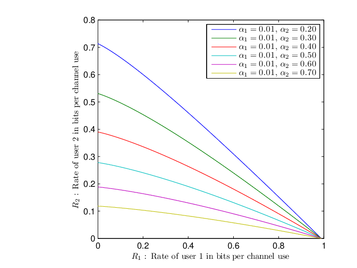
Figure 2 shows several example capacity region boundaries computed using Theorem 3.

Proof:

For the binary-symmetric BC $X\rightarrow Y\rightarrow Z$ with $0<\alpha_{1}<\alpha_{2}<1/2$ , one has

$\displaystyle\phi(p,\lambda)$	$\displaystyle\overset{\Delta}{=}\phi\left([p,1-p]^{T},\lambda\right)$
	$\displaystyle=h_{m}\left(T_{ZX}\boldsymbol{q}\right)-\lambda h_{n}\left(T_{YX}\boldsymbol{q}\right)$
	$\displaystyle=h\left((1-\alpha_{2})p+\alpha_{2}(1-p)\right)-\lambda h\left((1-\alpha_{1})p+\alpha_{1}(1-p)\right).$	(32)

Taking the second derivative of $\phi(p,\lambda)$ with respect to $p$ , we have

	$\displaystyle\phi^{\prime\prime}(p,\lambda)=\frac{-(1-2\alpha_{2})^{2}}{\left(\alpha_{2}p+(1-\alpha_{2})(1-p)\right)\left((1-\alpha_{2})p+\alpha_{2}(1-p)\right)}$
	$\displaystyle+\frac{\lambda(1-2\alpha_{1})^{2}}{\left(\alpha_{1}p+(1-\alpha_{1})(1-p)\right)\left((1-\alpha_{1})p+\alpha_{1}(1-p)\right)}\,.$		(33)

In (33), $\phi^{\prime\prime}(p,\lambda)=-A+\lambda B$ where $A$ and $B$ are both positive. Thus $\phi^{\prime\prime}(p,\lambda)$ has the sign of

\rho(p,\lambda)=\frac{\phi^{\prime\prime}(p,\lambda)}{AB}=-\left(\frac{1-\alpha_{1}}{1-2\alpha_{1}}-p\right)\left(\frac{\alpha_{1}}{1-2\alpha_{1}}+p\right)+\lambda\left(\frac{1-\alpha_{2}}{1-2\alpha_{2}}-p\right)\left(\frac{\alpha_{2}}{1-2\alpha_{2}}+p\right).

(34)

For any $0\leq\lambda\leq 1$ , $p=1/2$ minimizes $\rho$ so that

\min_{p}\rho(p,\lambda)=\frac{\lambda}{4(1-2\alpha_{2})^{2}}-\frac{1}{4(1-2\alpha_{1})^{2}}.

(35)

Thus, for $\lambda\geq(1-2\alpha_{2})^{2}/(1-2\alpha_{1})^{2}$ , $\phi^{\prime\prime}(p,\lambda)\geq 0$ for all $0\leq p\leq 1$ , and so $\psi(p,\lambda)=\phi(p,\lambda)$ . In this case, the transmission strategy that maximizes $R_{1}$ also maximizes $R_{2}+\lambda R_{1}$ . Thus, the optimal transmission strategy has $l=1$ , which means $U$ is a constant.

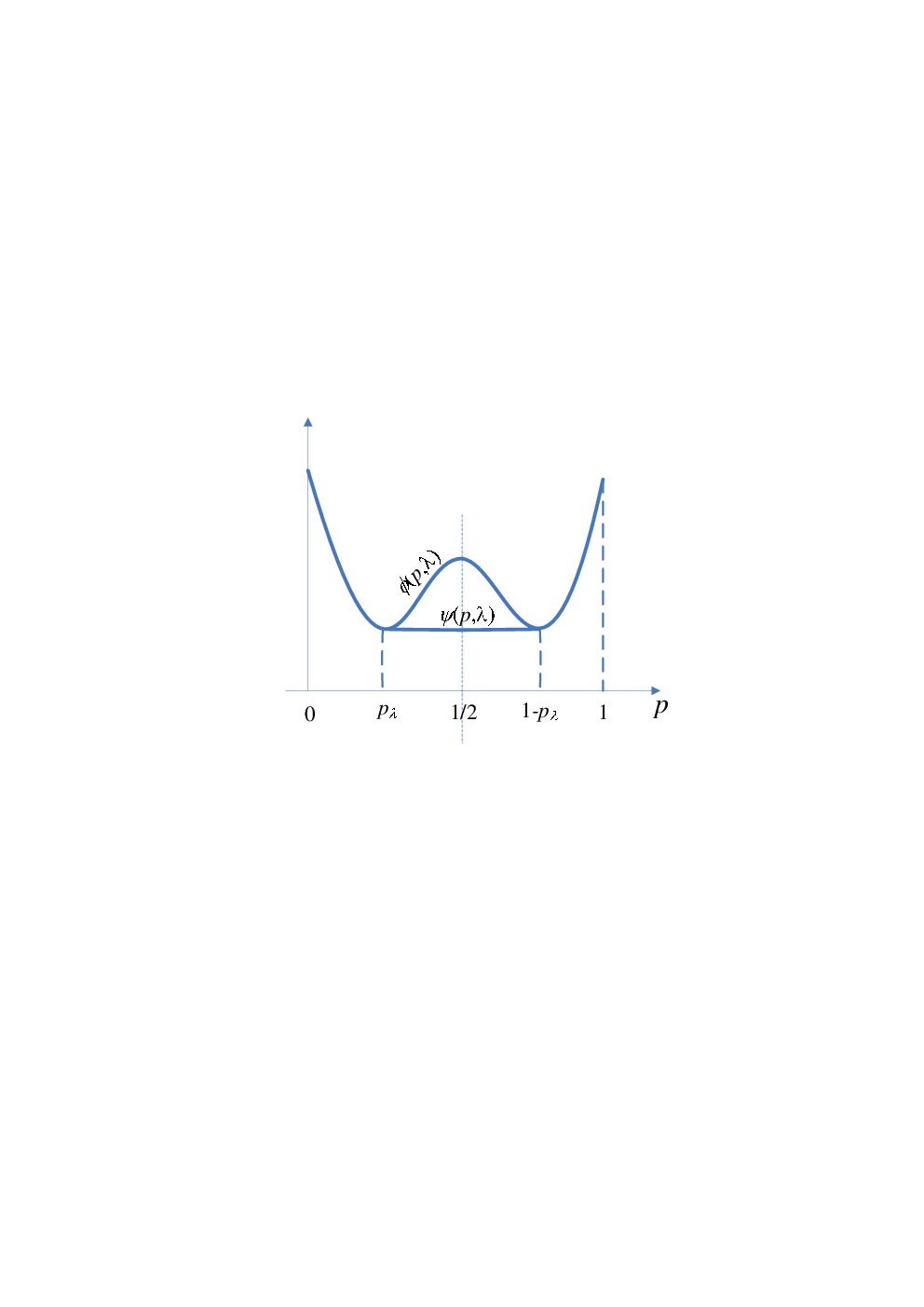
Note that $\phi(1/2+p,\lambda)=\phi(1/2-p,\lambda)$ . For $\lambda<(1-2\alpha_{2})^{2}/(1-2\alpha_{1})^{2}$ , $\phi(p,\lambda)$ has negative second derivative on an interval symmetric about $p=1/2$ . Let $p_{\lambda}=\arg\min_{p}\phi(p,\lambda)$ with $p_{\lambda}\leq 1/2$ . Thus $p_{\lambda}$ satisfies $\phi_{p}^{\prime}(p_{\lambda},\lambda)=0$ .

By symmetry, the envelope $\psi(\cdot,\lambda)$ is obtained by replacing $\phi(p,\lambda)$ on the interval $(p_{\lambda},1-p_{\lambda})$ by its minimum over $p$ , as shown in Figure 3. Therefore, the lower envelope of $\phi(p,\lambda)$ for the binary symmetric BC is

\psi(p,\lambda)=\left\{\begin{array}[]{ll}\phi(p_{\lambda},\lambda),&\textrm{for }p_{\lambda}\leq p\leq 1-p_{\lambda}\\ \phi(p,\lambda),&\textrm{otherwise}.\end{array}\right.

(36)

For a predetermined distribution of $X$ , $\boldsymbol{p}_{X}=\boldsymbol{q}=[q,1-q]^{T}$ with $p_{\lambda}<q<1-p_{\lambda}$ , the pair $(q,\psi(q,\lambda))$ is the convex combination of the points $(p_{\lambda},\phi(p_{\lambda},\lambda))$ and $(1-p_{\lambda},\phi(1-p_{\lambda},\lambda))$ . Therefore, by Theorem 2, the optimal transmission strategy with $\boldsymbol{p}_{X}=\boldsymbol{q}$ is NE with

\boldsymbol{p}_{U}=\left[\begin{array}[]{c}\frac{1-p_{\lambda}-q}{1-2p_{\lambda}}\\ \frac{q-p_{\lambda}}{1-2p_{\lambda}}\\ \end{array}\right]\text{ and }T_{XU}=\left[\begin{array}[]{cc}p_{\lambda}&1-p_{\lambda}\\ 1-p_{\lambda}&p_{\lambda}\\ \end{array}\right].

(37)

The conditional entropy bound $F^{*}(\boldsymbol{q},s)=h_{2}(T_{ZX}\cdot[p_{\lambda},1-p_{\lambda}]^{T})=h(\alpha_{2}+(1-2\alpha_{2})p_{\lambda})$ for $s=h_{2}(T_{YX}\cdot[p_{\lambda},1-p_{\lambda}]^{T})=h(\alpha_{1}+(1-2\alpha_{1})p_{\lambda})$ , and $p_{\lambda}\leq q\leq 1-p_{\lambda}$ . For the given $\boldsymbol{q}$ , this defines $F^{*}(s)\triangleq F^{*}(\boldsymbol{q},s)$ on its entire domain $s\in[h(\alpha_{1}),h(\alpha_{1}+(1-2\alpha_{1})q)]$ , i.e., $s\in$ $[H(Y|X),H(Y)]$ .

Note that for a predetermined distribution of $X$ , $\boldsymbol{p}_{X}=\boldsymbol{q}=[q,1-q]^{T}$ with the suboptimal choices of $q<p_{\lambda}$ or $q>1-p_{\lambda}$ , one has $\phi(q,\lambda)=\psi(q,\lambda)$ , which means that a line with slope $\lambda$ supports $F^{*}(\boldsymbol{q},\cdot)$ at point $s=H(Y)=h(\alpha_{1}+(1-2\alpha_{1})q)$ , and thus the optimal transmission strategy under the constraint that $q<p_{\lambda}$ or $q>1-p_{\lambda}$ has $l=1$ , which means $U$ is a constant.

The boundary of the capacity region for the binary-symmetric BC is always achieved when $\boldsymbol{p}_{X}=[1/2,1/2]^{T}$ (see [2]). Hence, the optimal transmission strategy to achieve the boundary of the capacity region always has $l=2$ and follows from (37) with $q=1/2$ . This leads to the following explicit parametric expression for the boundary of the capacity region of the two-receiver binary-symmetric BC:

		$\displaystyle R_{1}=h\left(\alpha_{1}+(1-2\alpha_{1})p_{\lambda}\right)-h(\alpha_{1}),$		(38)
		$\displaystyle R_{2}=\ln(2)-h\left(\alpha_{2}+(1-2\alpha_{2})p_{\lambda}\right),$		(39)

where the parameter $p_{\lambda}$ is ranging from 0 to 1/2. In addition, the rate pair $(R_{1},R_{2})$ in (38) and (39) maximizes $R_{2}+\lambda R_{1}$ for each pair of $\lambda$ and $p_{\lambda}$ satisfying $\phi_{p}^{\prime}(p_{\lambda},\lambda)=0$ , which implies

\displaystyle\lambda=\frac{1-2\alpha_{2}}{1-2\alpha_{1}}\cdot\frac{\ln{\frac{1-\alpha_{2}-(1-2\alpha_{2})p_{\lambda}}{\alpha_{2}+(1-2\alpha_{2})p_{\lambda}}}}{\ln{\frac{1-\alpha_{1}-(1-2\alpha_{1})p_{\lambda}}{\alpha_{1}+(1-2\alpha_{1})p_{\lambda}}}}.

∎

IV Broadcast Z Channels

The Z channel, shown in Figure 4(a), is a binary asymmetric channel which is noiseless when symbol 1 is transmitted but noisy when symbol 0 is transmitted. The channel output $Y$ is the binary OR of the channel input $X$ and Bernoulli distributed noise with parameter $\alpha$ . The capacity of the Z channel was studied in [19]. The Broadcast Z channel is a class of discrete memoryless broadcast channels whose component channels are Z channels. A two-receiver broadcast Z channel with marginal transition probability matrices

T_{YX}=\begin{bmatrix}1&\alpha_{1}\\ 0&1-\alpha_{1}\end{bmatrix},T_{ZX}=\begin{bmatrix}1&\alpha_{2}\\ 0&1-\alpha_{2}\end{bmatrix},

(40)

where $0<\alpha_{1}\leq\alpha_{2}<1$ , is shown in Fig 4(b). The two-receiver broadcast Z channel is stochastically degraded and can be modeled as a physically degraded broadcast channel as shown in Figure 5, where $\alpha_{\Delta}=(\alpha_{2}-\alpha_{1})/(1-\alpha_{1})$ [11]. NE for broadcast Z channels uses the binary OR function to combine each receiver’s independently encoded message. As shown in [11] [12], NE achieves the entire boundary of the capacity region for the two-receiver broadcast Z channel. In this section, we will show that NE also achieves the entire boundary of the capacity region for broadcast Z channels with more than two receivers.

IV-A Capacity region for the two-receiver broadcast Z channel

Similar to Theorem 3 for the BS broadcast channel, we can apply our analysis of $F^{*}$ to obtain a parametric expression for the capacity region of the broadcast Z channel.

Theorem 4

Consider the broadcast Z channel with crossover probabilities $0<\alpha_{1}\leq\alpha_{2}<1$ . Define $\beta_{i}=1-\alpha_{i}$ for $i=1,2$ . For $\lambda\geq 0$ , the achievable rate pair $(R_{1},R_{2})$ which maximizes $\lambda R_{1}+R_{2}$ is given by

	$\displaystyle R_{1}$	$\displaystyle=\frac{q_{\lambda}}{p_{\lambda}}h(\beta_{1}p_{\lambda})-q_{\lambda}h(\beta_{1}),$		(41)
	$\displaystyle R_{2}$	$\displaystyle=h(q_{\lambda}\beta_{2})-\frac{q_{\lambda}}{p_{\lambda}}h(\beta_{2}p_{\lambda}),$		(42)

where $\lambda$ , $q_{\lambda}$ , $R_{1}$ , and $R_{2}$ are parametrized by $0\leq p_{\lambda}\leq 1$ satisfying

	$\displaystyle\lambda$	$\displaystyle=\frac{\ln(1-\beta_{2}p_{\lambda})}{\ln(1-\beta_{1}p_{\lambda})}$		(43)
	$\displaystyle q_{\lambda}$	$\displaystyle=\min\left(p_{\lambda},\frac{1}{\beta_{2}\left(1+\exp\left({\frac{1}{\beta_{2}p_{\lambda}}\left(h(\beta_{2}p_{\lambda})-\lambda h(\beta_{1}p_{\lambda})+\lambda p_{\lambda}h(\beta_{1})\right)}\right)\right)}\right).$		(44)

Moreover, NE achieves all points in the capacity region.

Thus, Theorem 4 implies that for a specified $\alpha_{1}$ and $\alpha_{2}$ , the capacity region for the two-receiver broadcast Z channel can be determined parametrically for each $\lambda$ as follows:

1.

Use (43) to compute $p_{\lambda}$ from $\lambda$ .
2.

Use (44) to compute $q_{\lambda}$ from $p_{\lambda}$ .
3.

Use $q_{\lambda}$ and $p_{\lambda}$ in (41) and (42) to find the $R_{1}$ and $R_{2}$ that maximize $R_{2}+\lambda R_{1}$ .

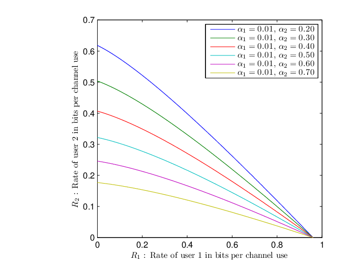
Figure 6 shows several example capacity region boundaries found using this procedure.

Proof:

For the broadcast Z channel $X\rightarrow Y\rightarrow Z$ shown in Figure 4(b) and Figure 5 with

T_{YX}=\begin{bmatrix}1&\alpha_{1}\\ 0&\beta_{1}\end{bmatrix},T_{ZX}=\begin{bmatrix}1&\alpha_{2}\\ 0&\beta_{2}\end{bmatrix},

(45)

where $0<\alpha_{1}\leq\alpha_{2}<1$ , $\beta_{1}=1-\alpha_{1}$ , and $\beta_{2}=1-\alpha_{2}$ , one has

\phi(p,\lambda)\overset{\Delta}{=}\phi\left([1-p,p]^{T},\lambda\right)=h(p\beta_{2})-\lambda h(p\beta_{1}).

(46)

Taking the second derivative of $\phi(p,\lambda)$ with respect to $p$ , we have

\phi^{\prime\prime}(p,\lambda)=\frac{-\beta_{2}}{(1-p\beta_{2})p}+\frac{\lambda\beta_{1}}{(1-p\beta_{1})p},

(47)

Multiplying $\phi^{\prime\prime}(p,\lambda)$ in (47) by the positive quantity $(1-p\beta_{1})(1-p\beta_{2})p$ produces

\rho(p,\lambda)=\phi^{\prime\prime}(p,\lambda)\cdot(1-p\beta_{1})(1-p\beta_{2})p=p\beta_{1}\beta_{2}(1-\lambda)+\lambda\beta_{1}-\beta_{2},

(48)

which has the same sign as $\phi^{\prime\prime}(p,\lambda)$ .

Let $\beta_{\Delta}\overset{\Delta}{=}\beta_{2}/\beta_{1}$ . For the case of $\beta_{\Delta}\leq\lambda\leq 1$ , $\phi^{\prime\prime}(p,\lambda)\geq 0$ for all $0\leq p\leq 1$ . Hence, $\phi(p,\lambda)$ is convex in $p$ and thus $\phi(p,\lambda)=\psi(p,\lambda)$ for all $0\leq p\leq 1$ . In this case, the transmission strategy that maximizes $R_{1}$ also maximizes $R_{2}+\lambda R_{1}$ . Thus, the optimal transmission strategy has $l=1$ , i.e., $U$ is a constant. Note that the transmission strategy with $l=1$ is a special case of the NE scheme in which the only codeword for the second receiver is an all-ones codeword.

For the case of $0\leq\lambda<\beta_{\Delta}$ , $\phi(p,\lambda)$ is concave in $p$ on $[0,\frac{\beta_{2}-\lambda\beta_{1}}{\beta_{1}\beta_{2}(1-\lambda)}]$ and convex on $[\frac{\beta_{2}-\lambda\beta_{1}}{\beta_{1}\beta_{2}(1-\lambda)},1]$ . Figure 7 illustrates the graph in this case. Since $\phi(0,\lambda)=0$ , $\psi(\cdot,\lambda)$ , the lower convex envelope of $\phi(\cdot,\lambda)$ , is constructed using the tangent of $\phi(\cdot,\lambda)$ that passes through the origin as shown in Figure 7. Let $(p_{\lambda},\phi(p_{\lambda},\lambda))$ be the point of contact. The value of $p_{\lambda}$ is determined by $\phi_{p}^{\prime}(p_{\lambda},\lambda)=\phi(p_{\lambda},\lambda)/p_{\lambda}$ , i.e.,

\lambda=\frac{\ln(1-\beta_{2}p_{\lambda})}{\ln(1-\beta_{1}p_{\lambda})}.

(49)

Let $\boldsymbol{q}=[1-q,q]^{T}$ be the distribution of the channel input $X$ . For $q\leq p_{\lambda}$ , $\psi(q,\lambda)$ is obtained as a convex combination of points $(0,0)$ and $(p_{\lambda},\phi(p_{\lambda},\lambda))$ with weights $(p_{\lambda}-q)/p_{\lambda}$ and $q/p_{\lambda}$ . By Theorem 2, it corresponds to $s=[(p_{\lambda}-q)/p_{\lambda}]\cdot 0+[q/p_{\lambda}]\cdot h(\beta_{1}p_{\lambda})=qh(\beta_{1}p_{\lambda})/p_{\lambda}$ and $F^{*}(q,s)\triangleq F^{*}(\boldsymbol{q},s)=q/p_{\lambda}\cdot h(\beta_{2}p_{\lambda})$ . Hence, for the broadcast Z channel,

F^{*}_{T_{YX},T_{ZX}}(q,qh(\beta_{1}p)/p)=qh(\beta_{2}p)/p

(50)

for $p\in[q,1]$ , which defines $F^{*}_{T_{YX},T_{ZX}}(q,\cdot)$ on its entire domain $[qh(\beta_{1}),h(q\beta_{1})]$ . Also by Theorem 2, the optimal transmission strategy $p(u,x)$ to maximize $(R_{2}+\lambda R_{1})$ given the constraint $\boldsymbol{p}_{X}=\boldsymbol{q}$ is determined by $l=2$ , $w_{1}=(p_{\lambda}-q)/p_{\lambda}$ , $w_{2}=q/p_{\lambda}$ , $\boldsymbol{t}_{1}=[1,0]^{T}$ and $\boldsymbol{t}_{2}=[1-p_{\lambda},p_{\lambda}]^{T}$ . Since the optimal transmission strategy $p(u,x)$ can be modeled as a Z channel as shown in Figure 8, the random variable $X$ can be constructed as the OR of two Bernoulli random variables with parameters $(p_{\lambda}-q)/p_{\lambda}$ and $1-p_{\lambda}$ respectively. Hence, an optimal transmission strategy for the broadcast Z channel is NE. For $q>p_{\lambda}$ , $\psi(q,\lambda)=\phi(q,\lambda)$ and an optimal strategy has $l=1$ , i.e., $U$ is a constant.

Thus, the two-receiver broadcast Z channel capacity region is the convex hull of the rate pairs $(R_{1},R_{2})$ satisfying

		$\displaystyle 0\leq R_{1}\leq\frac{q}{p_{\lambda}}h(\beta_{1}p_{\lambda})-qh(\beta_{1}),$		(51)
		$\displaystyle 0\leq R_{2}\leq h(q\beta_{2})-\frac{q}{p_{\lambda}}h(\beta_{2}p_{\lambda}),$		(52)

for some $q\in[0,1]$ and $p_{\lambda}\in[q,1]$ . For a fixed input distribution $\boldsymbol{p}_{X}=[1-q,q]^{T}$ , the rate pair $(R_{1},R_{2})$ of

		$\displaystyle R_{1}=\frac{q}{p_{\lambda}}h(\beta_{1}p_{\lambda})-qh(\beta_{1}),$		(53)
		$\displaystyle R_{2}=h(q\beta_{2})-\frac{q}{p_{\lambda}}h(\beta_{2}p_{\lambda}),$		(54)

maximizes $R_{2}+\lambda R_{1}$ for each pair of $\lambda$ and $p_{\lambda}$ satisfying (49). Among all possible input distributions $q\in[0,1]$ , only one will finally maximize $R_{2}+\lambda R_{1}$ over all rate pairs in the capacity region. Let $q_{\lambda}$ be the input distribution which maximizes $R_{2}+\lambda R_{1}$ , and thus,

$\displaystyle q_{\lambda}$	$\displaystyle=\arg\max_{0\leq q\leq p_{\lambda}}(R_{2}+\lambda R_{1})$	(55)
	$\displaystyle=\arg\max_{0\leq q\leq p_{\lambda}}\left(h(q\beta_{2})-\frac{q}{p_{\lambda}}h(\beta_{2}p_{\lambda})+\lambda\left(\frac{q}{p_{\lambda}}h(\beta_{1}p_{\lambda})-qh(\beta_{1})\right)\right),$	(56)
	$\displaystyle=\min\left(p_{\lambda},\frac{1}{\beta_{2}\left(1+\exp\left({\frac{1}{\beta_{2}p_{\lambda}}\left(h(\beta_{2}p_{\lambda})-\lambda h(\beta_{1}p_{\lambda})+\lambda p_{\lambda}h(\beta_{1})\right)}\right)\right)}\right).$	(57)

∎

IV-B The broadcast Z channel with more than two receivers

Consider a $K$ -receiver broadcast Z channel $X\rightarrow Y^{(1)}\rightarrow\cdots\rightarrow Y^{(K)}$ with marginal transition probability matrices

T_{Y_{j}X}=\begin{bmatrix}1&\alpha_{j}\\ 0&\beta_{j}\end{bmatrix},

(58)

where $0<\alpha_{1}\leq\cdots\leq\alpha_{K}<1$ , and $\beta_{j}=1-\alpha_{j}$ for $j=1,\cdots,K$ . The $K$ -receiver broadcast Z channel is stochastically degraded and can be modeled as a physically DBC as shown in Figure 9. NE for the $K$ -receiver broadcast Z channel combines the $K$ independently generated codewords (one for each receiver) using the binary OR operation. The $j^{\textrm{th}}$ receiver then successively decodes the messages for Receiver $K$ , Receiver $K-1$ , $\cdots$ , and finally for Receiver $j$ . The codebook for the $j^{\textrm{th}}$ receiver is a random codebook drawn according to the binary random variable $X^{(j)}$ with $\text{Pr}\{X^{(j)}=0\}=q^{(j)}$ . Denote $X^{(i)}\circ X^{(j)}$ as the binary OR of $X^{(i)}$ and $X^{(j)}$ . Hence, the channel input $X$ is the OR of $X^{(j)}$ for all $1\leq j\leq K$ , i.e., $X=X^{(1)}\circ\cdots\circ X^{(K)}$ . From the analysis of successive decoding in the proof of the coding theorem for DBCs [2] [3], the achievable region of NE for the $K$ -receiver broadcast Z channel is determined by

$\displaystyle R_{j}$	$\displaystyle\leq I\left(Y^{(j)},X^{(j)}\|X^{(j+1)},\cdots,X^{(K)}\right)$	(59)
	$\displaystyle=H\left(Y^{(j)}\|X^{(j+1)},\cdots,X^{(K)}\right)-H\left(Y^{(j)}\|X^{(j)},X^{(j+1)},\cdots,X^{(K)}\right)$	(60)
	$\displaystyle=\left(\prod_{i=j+1}^{K}q^{(i)}\right)\cdot h\left(\beta_{j}\prod_{i=1}^{j}q^{(i)}\right)-\left(\prod_{i=j}^{K}q^{(i)}\right)\cdot h\left(\beta_{j}\prod_{i=1}^{j-1}q^{(i)}\right)$	(61)
	$\displaystyle=\frac{q}{t_{j}}h(\beta_{j}t_{j})-\frac{q}{t_{j-1}}h(\beta_{j}t_{j-1}),$	(62)

where $t_{j}=\prod_{i=1}^{j}q^{(i)}$ for $j=1,\cdots,K$ , and $q=\textrm{Pr}(X=0)=\prod_{i=1}^{K}q^{(i)}$ . Denote $t_{0}=1$ . Since $0\leq q^{(1)},\cdots,q^{(K)}\leq 1$ , one has

1=t_{0}\geq t_{1}\geq\cdots\geq t_{K}=q.

(63)

Theorem 5 below states that NE achieves the entire boundary of the capacity region for broadcast Z channels with any finite number of receivers. Consider the communication system for the $K$ -receiver broadcast Z channel in Figure 10. $\boldsymbol{X}=(X_{1},\cdots,X_{N})$ is a length- $N$ codeword determined by the messages $W_{1},\cdots,W_{K}$ . $\boldsymbol{Y}^{(1)},\cdots,\boldsymbol{Y}^{(K)}$ are the channel outputs corresponding to the channel input $\boldsymbol{X}$ .

Theorem 5

If $\sum_{i=1}^{N}\text{Pr}\{X_{i}=0\}/N=q$ , then no point $(R_{1},\cdots,R_{K})$ such that

\begin{cases}R_{j}\geq\frac{q}{t_{j}}h(\beta_{j}t_{j})-\frac{q}{t_{j-1}}h(\beta_{j}t_{j-1}),\quad j=1,\cdots,K\\ R_{d}=\frac{q}{t_{d}}h(\beta_{d}t_{d})-\frac{q}{t_{d-1}}h(\beta_{d}t_{d-1})+\delta,\quad\textrm{for some }d\in\{1,\cdots,K\},\delta>0\end{cases}

(64)

is achievable, where the $t_{j}$ are as in (62) and (63).

Theorem 5 indicates that no rate point $(R_{1},\cdots,R_{K})$ outside the achievable region of the NE scheme is achievable because if there exists an achievable rate point $(R_{1},\cdots,R_{K})$ outside the NE scheme’s achievable region determined by (62), then there must exist a boundary point $(R^{*}_{1},\cdots,R^{*}_{K})$ on the NE scheme’s achievable region such that $R_{j}\geq R^{*}_{j}$ for all $j=1,\cdots,K$ , and $R_{d}>R^{*}_{d}$ for some $d\in\{1,\cdots,K\}$ .

The proof of Theorem 5 uses the same basic approach as the proof of the converse of the coding theorem for Gaussian BCs [2]. Lemma 1 below plays the same role in this proof as the entropy power inequality does in the proof for Gaussian BCs. We state and prove Lemma 1 and then proceed with the proof of Theorem 5.

Lemma 1

Consider the Markov chain $U\rightarrow\boldsymbol{X}\rightarrow\boldsymbol{Y}\rightarrow\boldsymbol{Z}$ with $\sum_{i=1}^{N}\text{Pr}(X_{i}=0)/N=q$ , if

H(\boldsymbol{Y}|U)\geq N\cdot\frac{q}{p}\cdot h(\beta_{1}p),

(65)

for some $p\in[q,1]$ , then

	$\displaystyle H(\boldsymbol{Z}\|U)$	$\displaystyle\geq N\cdot\frac{q}{p}\cdot h(\beta_{2}p)$		(66)
		$\displaystyle=N\cdot\frac{q}{p}\cdot h(\beta_{1}p\beta_{\Delta}).$		(67)

Proof:

Lemma 1 is the consequence of Proposition 9 for the broadcast Z channel. Since $H(\boldsymbol{Y}|U)\geq N\cdot q/p\cdot h(\beta_{1}p)$ ,

$\displaystyle H(\boldsymbol{Z}\|U)$	$\displaystyle\geq F^{*}_{T_{YX}^{(N)},T_{ZX}^{(N)}}(q,N\cdot q/p\cdot h(\beta_{1}p))$	(68)
	$\displaystyle=N\cdot F^{*}_{T_{YX},T_{ZX}}(q,q/p\cdot h(\beta_{1}p))$	(69)
	$\displaystyle=N\cdot\frac{q}{p}\cdot h(\beta_{2}p)$	(70)
	$\displaystyle=N\cdot\frac{q}{p}\cdot h(\beta_{1}p\beta_{\Delta}).$	(71)

These steps are justified as follows:

•

(68) follows from the definition of $F^{*}_{T_{YX}^{(N)},T_{ZX}^{(N)}}(\boldsymbol{q},s)$ ;
•

(69) follows from Proposition 9;
•

(70) follows from the expression of the function $F^{*}$ for the broadcast Z channel in (50);
•

(71) follows from $\beta_{\Delta}=\text{Pr}\{Z=0|Y=0\}=\beta_{2}/\beta_{1}$ .

∎

Proof:

The proof is by contradiction. To this end, suppose that the rates of (64) are achievable, which means that the probability of decoding error for each receiver can be upper bounded by an arbitrarily small $\epsilon$ for sufficiently large $N$

\textrm{Pr}\{\hat{W}_{j}\neq W_{j}|\boldsymbol{Y}^{(j)}\}<\epsilon,\quad j=1,\cdots,K.

(72)

By Fano’s inequality, this implies that

H(W_{j}|\boldsymbol{Y}^{(j)})\leq h(\epsilon)+\epsilon\ln(M_{j}-1),\quad j=1,\cdots,K.

(73)

Let $o(\epsilon)$ represent any function of $\epsilon$ such that $o(\epsilon)\geq 0$ and $o(\epsilon)\rightarrow 0$ as $\epsilon\rightarrow 0$ . Equation (73) implies that $H(W_{j}|\boldsymbol{Y}^{(j)})$ , $j=1,\cdots,K$ , are all $o(\epsilon)$ . Therefore,

$\displaystyle H(W_{j})$	$\displaystyle=H(W_{j}\|W_{j+1},\cdots,W_{K})$	(74)
	$\displaystyle=I(W_{j};\boldsymbol{Y}^{(j)}\|W_{j+1},\cdots,W_{K})+H(W_{j}\|\boldsymbol{Y}^{(j)},W_{j+1},\cdots,W_{K})$	(75)
	$\displaystyle\leq I(W_{j};\boldsymbol{Y}^{(j)}\|W_{j+1},\cdots,W_{K})+H(W_{j}\|\boldsymbol{Y}^{(j)})$	(76)
	$\displaystyle=H(\boldsymbol{Y}^{(j)}\|W_{j+1},\cdots,W_{K})-H(\boldsymbol{Y}^{(j)}\|W_{j},W_{j+1},\cdots,W_{K})+o(\epsilon),$	(77)

where (74) follows from the independence of the $W_{j}$ , $j=1,\cdots,K$ . From (64), (77) and the fact that $NR_{j}\leq H(W_{j})$ ,

H(\boldsymbol{Y}^{(j)}|W_{j+1},\cdots,W_{K})-H(\boldsymbol{Y}^{(j)}|W_{j},W_{j+1},\cdots,W_{K})\geq N\frac{q}{t_{j}}h(\beta_{j}t_{j})-N\frac{q}{t_{j-1}}h(\beta_{j}t_{j-1})-o(\epsilon).

(78)

Next, using Lemma 1 and (78), we show in Appendix B that

H(\boldsymbol{Y}^{(K)})\geq Nh(\beta_{K}q)+N\delta-o(\epsilon),

(79)

where $q=t_{K}=\sum_{i=1}^{N}\textrm{Pr}(X_{i}=0)/N$ . Since $\epsilon$ can be arbitrarily small for sufficient large $N$ , $o(\epsilon)\rightarrow 0$ as $N\rightarrow\infty$ . For sufficiently large $N$ , $H(\boldsymbol{Y}^{(K)})\geq Nh(\beta_{K}q)+N\delta/2$ . However, this contradicts

$\displaystyle H(\boldsymbol{Y}^{(K)})$	$\displaystyle\leq\sum_{i=1}^{N}H(Y^{(K)}_{i})$	(80)
	$\displaystyle=\sum_{i=1}^{N}h\left(\beta_{K}\cdot\textrm{Pr}(X_{i}=0)\right)$	(81)
	$\displaystyle\leq Nh\left(\beta_{K}\cdot\sum_{i=1}^{N}\textrm{Pr}(X_{i}=0)/N\right)$	(82)
	$\displaystyle=Nh(\beta_{K}q).$	(83)

Some of these steps are justified as follows:

•

(80) follows from $\boldsymbol{Y}^{(K)}=(Y^{(K)}_{1},\cdots,Y^{(K)}_{N})$ ;
•

(82) is obtained by applying Jensen’s inequality to the concave function $h(\cdot)$ ;
•

(83) follows from $q=\sum_{i=1}^{N}\textrm{Pr}(X_{i}=0)/N$ .

The desired contradiction has been obtained, so the theorem is proved. ∎

V Input-Symmetric Degraded Broadcast Channels

The input-symmetric channel was first introduced in [9] and studied further in [15] [16] [20]. The definition of the input-symmetric channel is as follows: Let $\Phi_{n}$ denote the symmetric group of permutations of $n$ objects by $n\times n$ permutation matrices. An $n$ -input $m$ -output channel with transition probability matrix $T_{m\times n}$ is input-symmetric if the set

\mbox{$\mathcal{G}$}_{T}=\left\{G\in\Phi_{n}|\exists\Pi\in\Phi_{m},\text{ s.t. }TG=\Pi T\right\}

(84)

is transitive, which means for any $i,j\in\{1,\cdots,n\}$ , there exists a permutation matrix $G\in\mbox{$\mathcal{G}$}_{T}$ which maps the $i$ -th row to the $j$ -th row [9]. An important property of input-symmetric channels is that the uniform distribution achieves capacity. We extend the definition of the input-symmetric channel to the input-symmetric DBC as follows:

Definition 2

(Input-Symmetric Degraded Broadcast Channel) A discrete memoryless DBC $X\rightarrow Y\rightarrow Z$ with $|\mbox{$\mathcal{X}$}|=k$ , $|\mbox{$\mathcal{Y}$}|=n$ and $|\mbox{$\mathcal{Z}$}|=m$ is input-symmetric if the set $\mbox{$\mathcal{G}$}_{T_{YX},T_{ZX}}$ is transitive where

	$\displaystyle\mbox{$\mathcal{G}$}_{T_{YX},T_{ZX}}$	$\displaystyle\overset{\Delta}{=}\mbox{$\mathcal{G}$}_{T_{YX}}\cap\mbox{$\mathcal{G}$}_{T_{ZX}}$		(85)
		$\displaystyle=\left\{G\in\Phi_{k}\|\exists\Pi_{YX}\in\Phi_{n},\Pi_{ZX}\in\Phi_{m},\text{ s.t. }T_{YX}G=\Pi_{YX}T_{YX},T_{ZX}G=\Pi_{ZX}T_{ZX}\right\}\,.$		(86)

Lemmas 2 and 3 below establish basic properties of $\mbox{$\mathcal{G}$}_{T_{YX},T_{ZX}}$ .

Lemma 2

$\mbox{$\mathcal{G}$}_{T_{YX},T_{ZX}}$ is a group under matrix multiplication.

Proof:

Every closed subset of a group is a group. Since $\mbox{$\mathcal{G}$}_{T_{YX},T_{ZX}}$ is a subset of $\Phi_{k}$ , which is a group under matrix multiplication, it suffices to show that $\mbox{$\mathcal{G}$}_{T_{YX},T_{ZX}}$ is closed under matrix multiplication. Suppose $G_{1},G_{2}\in\mbox{$\mathcal{G}$}_{T_{YX},T_{ZX}}$ such that $T_{YX}G_{1}=\Pi_{YX,1}T_{YX}$ , $T_{ZX}G_{1}=\Pi_{ZX,1}T_{ZX}$ , $T_{YX}G_{2}=\Pi_{YX,2}T_{YX}$ and $T_{ZX}G_{2}=\Pi_{ZX,2}T_{ZX}$ . Thus,

T_{YX}G_{1}G_{2}=\Pi_{YX,1}\Pi_{YX,2}T_{YX},

(87)

and

T_{ZX}G_{1}G_{2}=\Pi_{ZX,1}\Pi_{ZX,2}T_{ZX}.

(88)

Therefore, $G_{1}G_{2}\in\mbox{$\mathcal{G}$}_{T_{YX},T_{ZX}}$ . ∎

Lemma 3

Let $l=|\mbox{$\mathcal{G}$}_{T_{YX},T_{ZX}}|$ so that $\mbox{$\mathcal{G}$}_{T_{YX},T_{ZX}}\overset{\Delta}{=}\mbox{$\mathcal{G}$}_{T_{YX}}\cap\mbox{$\mathcal{G}$}_{T_{ZX}}=\{G_{1},\cdots,G_{l}\}$ . Also let $k=|\mathcal{X}|$ . Then $\sum_{i=1}^{l}G_{i}=\frac{l}{k}\boldsymbol{1}\boldsymbol{1}^{T}$ , where $\frac{l}{k}$ is an integer and $\boldsymbol{1}$ is an all-ones vector.

Proof:

For all $j=1,\cdots,l$ ,

G_{j}\left(\sum_{i=1}^{l}G_{i}\right)\stackrel{{\scriptstyle(a)}}{{=}}\sum_{i=1}^{l}G_{j}G_{i}\stackrel{{\scriptstyle(b)}}{{=}}\sum_{i=1}^{l}G_{i},

(89)

where (a) follows from the distributive law for the field of rational matrices and (b) follows from the closure axiom and the inverse element axiom for the group $\mbox{$\mathcal{G}$}_{T_{YX},T_{ZX}}$ .

Hence, $\sum_{i=1}^{l}G_{i}$ has $k$ identical columns and $k$ identical rows since $\mbox{$\mathcal{G}$}_{T_{YX},T_{ZX}}$ is transitive. Therefore, $\sum_{i=1}^{l}G_{i}=\frac{l}{k}\boldsymbol{1}\boldsymbol{1}^{T}$ . ∎

Definition 3

(Smallest Transitive Set) A subset of $\mbox{$\mathcal{G}$}_{T_{YX},T_{ZX}}$ , $\{G_{i_{1}},\cdots,G_{i_{l_{s}}}\}$ , is a smallest transitive subset of $\mbox{$\mathcal{G}$}_{T_{YX},T_{ZX}}$ if

\sum_{j=1}^{l_{s}}G_{i_{j}}=\frac{l_{s}}{k}\boldsymbol{1}\boldsymbol{1}^{T},

(90)

where $\frac{l_{s}}{k}$ is the smallest possible integer for which (90) is satisfied.

V-A Examples: binary-symmetric BCs and binary-erasure BCs

The class of input-symmetric DBCs includes most of the common discrete memoryless DBCs. For example, the binary-symmetric BC $X\rightarrow Y\rightarrow Z$ with marginal transition probability matrices

T_{YX}=\begin{bmatrix}1-\alpha_{1}&\alpha_{1}\\ \alpha_{1}&1-\alpha_{1}\end{bmatrix}\text{ and }T_{ZX}=\begin{bmatrix}1-\alpha_{2}&\alpha_{2}\\ \alpha_{2}&1-\alpha_{2}\end{bmatrix},

where $0\leq\alpha_{1}\leq\alpha_{2}\leq 1/2$ , is input-symmetric since

\mbox{$\mathcal{G}$}_{T_{YX},T_{ZX}}=\left\{\begin{bmatrix}1&0\\ 0&1\end{bmatrix},\begin{bmatrix}0&1\\ 1&0\end{bmatrix}\right\}

(91)

is transitive.

Another interesting example is the binary-erasure BC with marginal transition probability matrices

T_{YX}=\begin{bmatrix}1-a_{1}&0\\ a_{1}&a_{1}\\ 0&1-a_{1}\end{bmatrix}\text{ and }T_{ZX}=\begin{bmatrix}1-a_{2}&0\\ a_{2}&a_{2}\\ 0&1-a_{2}\end{bmatrix},

where $0\leq a_{1}\leq a_{2}\leq 1$ . It is input-symmetric since its $\mbox{$\mathcal{G}$}_{T_{YX},T_{ZX}}$ is the same as that of the binary-symmetric BC shown in (91).

V-B Group-Operation DBCs are input-symmetric.

We now define group-operation DBCs and show that they are input symmetric.

Definition 4

(Group-Operation Degraded Broadcast Channel) A discrete DBC $X\rightarrow Y\rightarrow Z$ with $\mathcal{X,Y,Z}$ $=\{1,\cdots,n\}$ is a group-operation DBC if there exist two $n$ -ary random variables $N_{1}$ and $N_{2}$ such that $Y\sim X\oplus N_{1}$ and $Z\sim Y\oplus N_{2}$ as shown in Figure 11, where $\sim$ denotes identical distribution and $\oplus$ denotes a group operation which is an operation that satisfies the group axioms on the set $\{1,\cdots,n\}$ .

Group-operation DBCs include the binary-symmetric BC and the discrete additive DBC of [10] as special cases. It is also a channel model for Gaussian broadcast communication systems with phase-shift-keying (PSK) modulation at the transmitter and direct hard decisions on modulated symbols at the receivers.

Theorem 6

Group-operation DBCs are input-symmetric.

Proof:

For the group-operation DBC $X\rightarrow Y\rightarrow Z$ with $\mathcal{X,Y,Z}$ $=\{1,\cdots,n\}$ , let $G_{x}$ for $x=1,\cdots,n$ , be 0-1 matrices with entries

G_{x}(i,j)=\begin{cases}1&\text{if $j\oplus x=i$}\\ 0&\text{otherwise}\end{cases}\,\text{for }i,j=1,\cdots,n.

(92)

$G_{x}$ for $x=1,\cdots,n$ , are actually permutation matrices and have the property that $G_{x_{1}}\cdot G_{x_{2}}=G_{x_{2}}\cdot G_{x_{1}}=G_{x_{1}\oplus x_{2}}$ . Let $[\gamma_{1},\cdots,\gamma_{n}]^{T}$ be the distribution of $N_{1}$ . Since $Y$ has the same distribution as $X\oplus N_{1}$ , one has

T_{YX}=\sum_{x=1}^{n}\gamma_{x}G_{x}.

(93)

Hence, $T_{YX}G_{x}=G_{x}T_{YX}$ for all $x=1,\cdots,n$ . Similarly, we have $T_{ZX}G_{x}=G_{x}T_{ZX}$ for all $x=1,\cdots,n$ , and so

\{G_{1},\cdots,G_{n}\}\subseteq\mbox{$\mathcal{G}$}_{T_{YX},T_{ZX}}.

(94)

Since the set $\{G_{1},\cdots,G_{n}\}$ is transitive by definition, $\mbox{$\mathcal{G}$}_{T_{YX},T_{ZX}}$ is also transitive and hence the group-operation DBC is input-symmetric. ∎

By definition, $\sum_{j=1}^{n}G_{j}=\boldsymbol{1}\boldsymbol{1}^{T}$ , and hence, $\{G_{1},\cdots,G_{n}\}$ is a smallest transitive subset of $\mbox{$\mathcal{G}$}_{T_{YX},T_{ZX}}$ for the group-operation DBC.

V-C A note on discrete degraded interference channels (DDICs)

We briefly note that while DDICs and their related DBCs are closely related to IS-DBCs, the class of IS-DBCs is not addressed by [15] or [16]. The class of DDICs and the corresponding DBCs studied in [15] and [16] have to satisfy the condition that the transition probability matrix $T_{ZY}$ is input-symmetric, i.e., $\mbox{$\mathcal{G}$}_{T_{ZY}}$ is transitive. The input-symmetric DBC, however, does not have to satisfy this condition. The following example provides an IS-DBC which is not covered in [15] [16]. Consider a binary-input DBC $X\rightarrow Y\rightarrow Z$ with transition probability matrices

T_{YX}=\begin{bmatrix}a&c\\ b&d\\ c&a\\ d&b\end{bmatrix},T_{ZY}=\begin{bmatrix}e&f&g&h\\ g&h&e&f\end{bmatrix},

and

T_{ZX}=T_{ZY}T_{YX}=\begin{bmatrix}\alpha&\beta\\ \beta&\alpha\\ \end{bmatrix},

(95)

where $a+c=b+d=1$ , $e+f+g+h=1$ , $\alpha=ae+bf+cg+dh$ and $\beta=ag+bh+ce+df$ . This DBC is input-symmetric since its $\mbox{$\mathcal{G}$}_{T_{YX},T_{ZX}}$ is the same as that of the broadcast binary-symmetric channel shown in (91). It is not covered by the results of [15] [16] because

\mbox{$\mathcal{G}$}_{T_{ZY}}=\left\{\begin{bmatrix}1&0&0&0\\ 0&1&0&0\\ 0&0&1&0\\ 0&0&0&1\end{bmatrix},\begin{bmatrix}0&0&1&0\\ 0&0&0&1\\ 1&0&0&0\\ 0&1&0&0\end{bmatrix}\right\}

(96)

is not transitive.

V-D Optimal input distribution and capacity region for IS-DBCs

Consider the input-symmetric DBC $X\rightarrow Y\rightarrow Z$ with the marginal transition probability matrices $T_{YX}$ and $T_{ZX}$ . Recall that the set $\mathcal{C}$ is the set of all $(\boldsymbol{p}_{X},s,\eta)$ satisfying (2), (3) and (4) for some choice of $l$ , $\boldsymbol{w}$ and $T_{XU}$ , the set $\mathcal{C}^{*}$ $=\{(s,\eta)|(\boldsymbol{p}_{X},s,\eta)\in$ $\mathcal{C}$ $\text{ for some }\boldsymbol{p}_{X}\}$ is the projection of the set $\mathcal{C}$ on the $(s,\eta)$ -plane, and the set $\mathcal{C}^{*}_{\boldsymbol{q}}$ is the subset of $\mathcal{C}^{*}$ for which $\boldsymbol{p}_{X}=\boldsymbol{q}$ .

Lemma 4

For any permutation matrix $G\in\mbox{$\mathcal{G}$}_{T_{YX},T_{ZX}}$ and $(\boldsymbol{p},s,\eta)\in\mathcal{C}$ , $(G\boldsymbol{p},s,\eta)\in\mathcal{C}$ .

Proof:

Since $(\boldsymbol{p},s,\eta)$ satisfies (2), (3) and (4) for some choice of $l$ , $\boldsymbol{w}$ and $T_{XU}=[\boldsymbol{t}_{1}\cdots\boldsymbol{t}_{l}]$ ,

$\displaystyle GT_{XU}\boldsymbol{w}$	$\displaystyle=G\boldsymbol{p}$	(97)
$\displaystyle\sum_{j=1}^{l}w_{j}h_{n}(T_{YX}G\boldsymbol{t}_{j})$	$\displaystyle=\sum_{j=1}^{l}w_{j}h_{n}(\Pi_{YX}T_{YX}\boldsymbol{t}_{j})=s$	(98)
$\displaystyle\sum_{j=1}^{l}w_{j}h_{m}(T_{ZX}G\boldsymbol{t}_{j})$	$\displaystyle=\sum_{j=1}^{l}w_{j}h_{m}(\Pi_{ZX}T_{ZX}\boldsymbol{t}_{j})=\eta.$	(99)

Hence, $(G\boldsymbol{p},s,\eta)$ satisfies (2), (3) and (4) for the choice of $l$ , $\boldsymbol{w}$ and $GT_{XU}$ . ∎

Corollary 1

$\forall\boldsymbol{p}\in\Delta_{k}$ and $G\in\mbox{$\mathcal{G}$}_{T_{YX},T_{ZX}}$ , one has $\mbox{$\mathcal{C}$}^{*}_{G\boldsymbol{p}}=\mbox{$\mathcal{C}$}^{*}_{\boldsymbol{p}}$ , and so $F^{*}(G\boldsymbol{p},s)=F^{*}(\boldsymbol{p},s)$ for any $H(Y|X)\leq s\leq H(Y)$ .

Lemma 5

For any input-symmetric DBC, $\mbox{$\mathcal{C}$}^{*}=\mbox{$\mathcal{C}$}^{*}_{\boldsymbol{u}}$ , where $\boldsymbol{u}$ denotes the uniform distribution.

Proof:

For any $(s,\eta)\in\mbox{$\mathcal{C}$}^{*}$ , there exits a distribution $\boldsymbol{p}$ such that $(\boldsymbol{p},s,\eta)\in\mbox{$\mathcal{C}$}$ . Let $\mbox{$\mathcal{G}$}_{T_{YX},T_{ZX}}=\{G_{1},\cdots,G_{l}\}$ . By Corollary 1, $(G_{j}\boldsymbol{p},s,\eta)\in\mbox{$\mathcal{C}$}$ for all $j=1,\cdots,l$ . By the convexity of the set $\mathcal{C}$ ,

(\boldsymbol{q},s,\eta)=\left(\sum_{j=1}^{l}\frac{1}{l}G_{j}\boldsymbol{p}\;,s,\eta\right)\in\mathcal{C},

(100)

where $\boldsymbol{q}=\sum_{j=1}^{l}\frac{1}{l}G_{j}\boldsymbol{p}$ . Since $\mbox{$\mathcal{G}$}_{T_{YX},T_{ZX}}$ is a group , for any permutation matrix $G^{\prime}\in\mbox{$\mathcal{G}$}_{T_{YX},T_{ZX}}$ ,

G^{\prime}\boldsymbol{q}\;=\!\sum_{j=1}^{l}\!\!\frac{1}{l}G^{\prime}G_{j}\boldsymbol{p}\;=\!\sum_{j=1}^{l}\!\!\frac{1}{l}G_{j}\boldsymbol{p}\;=\;\boldsymbol{q}.

(101)

Since $G^{\prime}\boldsymbol{q}=\boldsymbol{q}$ , the $i^{\text{th}}$ entry and the $j^{\text{th}}$ entry of $\boldsymbol{q}$ are the same if $G^{\prime}$ permutes the $i^{\text{th}}$ row to the $j^{\text{th}}$ row. Since the set $\mbox{$\mathcal{G}$}_{T_{YX},T_{ZX}}$ for an input-symmetric DBC is transitive, all the entries of $\boldsymbol{q}$ are the same, and so $\boldsymbol{q}=\boldsymbol{u}$ . This implies that $(s,\eta)\in\mbox{$\mathcal{C}$}^{*}_{\boldsymbol{u}}$ . Since $(s,\eta)$ is arbitrarily taken from $\mbox{$\mathcal{C}$}^{*}$ , one has $\mbox{$\mathcal{C}$}^{*}\subseteq\mbox{$\mathcal{C}$}^{*}_{\boldsymbol{u}}$ . On the other hand, by definition, $\mbox{$\mathcal{C}$}^{*}\supseteq\mbox{$\mathcal{C}$}^{*}_{\boldsymbol{u}}$ . Therefore, $\mbox{$\mathcal{C}$}^{*}=\mbox{$\mathcal{C}$}^{*}_{\boldsymbol{u}}$ . ∎

Now we state and prove that the uniformly distributed $X$ is optimal for input-symmetric DBCs.

Theorem 7

For any input-symmetric DBC, its capacity region can be achieved by using the transmission strategies such that the broadcast signal $X$ is uniformly distributed. As a consequence, the capacity region is

\bar{\text{co}}\left\{(R_{1},R_{2}):R_{1}\leq s-h_{n}(T_{YX}\boldsymbol{e_{1}}),R_{2}\leq h_{m}(T_{ZX}\boldsymbol{u})-F^{*}_{T_{YX},T_{ZX}}(\boldsymbol{u},s),h_{n}(T_{YX}\boldsymbol{e_{1}})\leq s\leq\ln(n)\right\},

(102)

where $\boldsymbol{e_{1}}=[1,0,\cdots,0]^{T}$ , $n=|\mathcal{Y}|$ , and $m=|\mathcal{Z}|$ .

Proof:

Let $\boldsymbol{q}=[q_{1},\cdots,q_{k}]^{T}$ be the distribution of the channel input $X$ for the input-symmetric DBC $X\rightarrow Y\rightarrow Z$ . Since $\mbox{$\mathcal{G}$}_{T_{YX}}$ is transitive, the columns of $T_{YX}$ are permutations of each other.

$\displaystyle H(Y\|X)$	$\displaystyle=\sum_{i=1}^{k}q_{i}H(Y\|X=i)$	(103)
	$\displaystyle=\sum_{i=1}^{k}q_{i}h_{n}(T_{YX}\boldsymbol{e_{i}})$	(104)
	$\displaystyle=\sum_{i=1}^{k}q_{i}h_{n}(T_{YX}\boldsymbol{e_{1}})$	(105)
	$\displaystyle=h_{n}(T_{YX}\boldsymbol{e_{1}}),$	(106)

which is independent of $\boldsymbol{q}$ . Let $l=|\mbox{$\mathcal{G}$}_{T_{YX},T_{ZX}}|$ and $\mbox{$\mathcal{G}$}_{T_{YX},T_{ZX}}=\{G_{1},\cdots,G_{l}\}$ .

$\displaystyle H(Z)$	$\displaystyle=h_{m}(T_{ZX}\boldsymbol{q})$	(107)
	$\displaystyle=\frac{1}{l}\sum_{i=1}^{l}h_{m}(T_{ZX}G_{i}\boldsymbol{q})$	(108)
	$\displaystyle\leq h_{m}\left(T_{ZX}\sum_{i=1}^{l}\frac{1}{l}G_{i}\boldsymbol{q}\right)$	(109)
	$\displaystyle=h_{m}(T_{ZX}\boldsymbol{u}),$	(110)

where (109) follows from Jensen’s inequality. Since $\mbox{$\mathcal{C}$}^{*}=\mbox{$\mathcal{C}$}^{*}_{\boldsymbol{u}}$ for the input-symmetric DBC,

F^{*}(\boldsymbol{q},s)\geq F^{*}(\boldsymbol{u},s).

(111)

Plugging (106), (110) and (111) into (17), the expression of the capacity region for the DBC, the capacity region for input-symmetric DBCs is

	$\displaystyle\bar{\text{co}}\left[\bigcup_{\boldsymbol{p}_{X}=\boldsymbol{q}\in\Delta_{k}}\left\{(R_{1},R_{2}):R_{1}\leq s-H(Y\|X),R_{2}\leq H(Z)-F^{*}_{T_{YX},T_{ZX}}(\boldsymbol{q},s)\right\}\right]$	(112)
$\displaystyle\subseteq\;$	$\displaystyle\bar{\text{co}}\left[\bigcup_{\boldsymbol{p}_{X}=\boldsymbol{q}\in\Delta_{k}}\left\{(R_{1},R_{2}):R_{1}\leq s-h_{n}(T_{YX}\boldsymbol{e_{1}}),R_{2}\leq h_{m}(T_{ZX}\boldsymbol{u})-F^{*}_{T_{YX},T_{ZX}}(\boldsymbol{u},s)\right\}\right]$	(113)
$\displaystyle=\;$	$\displaystyle\bar{\text{co}}\left\{(R_{1},R_{2}):R_{1}\leq s-h_{n}(T_{YX}\boldsymbol{e_{1}}),R_{2}\leq h_{m}(T_{ZX}\boldsymbol{u})-F^{*}_{T_{YX},T_{ZX}}(\boldsymbol{u},s)\right\}$	(114)
$\displaystyle=\;$	$\displaystyle\bar{\text{co}}\left\{(R_{1},R_{2}):\boldsymbol{p}_{X}=\boldsymbol{u},R_{1}\leq s-H(Y\|X),R_{2}\leq H(Z)-F^{*}_{T_{YX},T_{ZX}}(\boldsymbol{u},s)\right\}$	(115)
$\displaystyle\subseteq$	$\displaystyle\bar{\text{co}}\left[\bigcup_{\boldsymbol{p}_{X}=\boldsymbol{q}\in\Delta_{k}}\left\{(R_{1},R_{2}):R_{1}\leq s-H(Y\|X),R_{2}\leq H(Z)-F^{*}_{T_{YX},T_{ZX}}(\boldsymbol{q},s)\right\}\right],$	(116)

Note that (112) and (116) are identical expressions, hence (112 - 116) are all equal. Therefore, (102) and (114) express the capacity region for the input-symmetric DBC, which also means that the capacity region can be achieved by using transmission strategies where the broadcast signal $X$ is uniformly distributed. ∎

V-E Permutation encoding approach and its optimality for IS-DBCs

The permutation encoding approach is an independent-encoding scheme which achieves the capacity region for input-symmetric DBCs. The block diagram of this approach is shown in Figure 12. In Figure 12, $W_{1}$ is the message for Receiver 1, which sees the less-degraded channel $T_{YX}$ , and $W_{2}$ is the message for Receiver 2, which sees the more-degraded channel $T_{ZX}$ . The permutation encoding approach is first to independently encode these two messages into two codewords $\boldsymbol{X}^{(1)}$ and $\boldsymbol{X}^{(2)}$ , and then to combine these two independent codewords using a single-letter operation.

Let $\mbox{$\mathcal{G}$}_{s}$ be a smallest transitive subset of $\mbox{$\mathcal{G}$}_{T_{YX},T_{ZX}}$ . Denote $k=|\mathcal{X}|$ and $l_{s}=|\mbox{$\mathcal{G}$}_{s}|$ . Use a random coding technique to design the codebook for Receiver 1 according to the $k$ -ary random variable $X^{(1)}$ with distribution $\boldsymbol{p_{1}}$ and the codebook for Receiver 2 according to the $l_{s}$ -ary random variable $X^{(2)}$ with uniform distribution. Let $\mbox{$\mathcal{G}$}_{s}=\{G_{1},\cdots,G_{l_{s}}\}$ . Define the permutation function $g_{x^{(2)}}(x^{(1)})=x$ if the permutation matrix $G_{x^{(2)}}$ maps the $x^{(1)}$ -th column to the $x$ -th column, where $x^{(2)}\in\{1,\cdots,l_{s}\}$ and $x,x^{(1)}\in\{1,\cdots,k\}$ . Hence, $g_{x^{(2)}}(x^{(1)})=x$ if and only if the $x^{(1)}$ -th row, $x$ -th column entry of $G_{x^{(2)}}$ is 1. The permutation encoding approach is then to broadcast $\boldsymbol{X}$ which is obtained by applying the single-letter permutation function $X=g_{X^{(2)}}(X^{(1)})$ on symbols of codewords $\boldsymbol{X}^{(1)}$ and $\boldsymbol{X}^{(2)}$ . Since $X^{(2)}$ is uniformly distributed and $\sum_{j=1}^{l_{s}}G_{j}=\frac{l_{s}}{k}\boldsymbol{1}\boldsymbol{1}^{T}$ , the broadcast signal $X$ is also uniformly distributed.

Receiver 2 receives $\boldsymbol{Z}$ and decodes the desired message directly. Receiver 1 receives $\boldsymbol{Y}$ and successively decodes the message for Receiver 2 and then for Receiver 1. The structure of the successive decoder is shown in Figure 13. Note that Decoder 1 in Figure 13 is not a joint decoder even though it has two inputs $\boldsymbol{Y}$ and $\boldsymbol{\hat{X}}^{(2)}$ .

In particular, for the group-operation DBC with $Y\sim X\oplus N_{1}$ and $Z\sim Y\oplus N_{2}$ , the permutation function $g_{x^{(2)}}(x^{(1)})$ is the group operation $x^{(2)}\oplus x^{(1)}$ . Hence the permutation encoding approach for the group-operation DBC is the NE scheme for the group-operation DBC. The successive decoder for the group-operation DBC is shown in Figure 14, where

\tilde{y}=y\oplus(-\hat{x}^{(2)}).

(117)

From the analysis of successive decoding in the proof of the coding theorem for DBCs [2] [3], the achievable region of the permutation encoding approach for the input-symmetric DBC is determined by

$\displaystyle R_{1}$	$\displaystyle\leq I(X;Y\|X^{(2)})$	(118)
	$\displaystyle=H(Y\|X^{(2)})-H(Y\|X)$	(119)
	$\displaystyle=\sum_{x^{(2)}=1}^{l_{s}}\text{Pr}(X^{(2)}=x^{(2)})H(Y\|X^{(2)}=x^{(2)})-\sum_{x=1}^{k}\text{Pr}(X=x)H(Y\|X=x)$	(120)
	$\displaystyle=\sum_{x^{(2)}=1}^{l_{s}}\text{Pr}(X^{(2)}=x^{(2)})h_{n}(T_{YX}G_{x^{(2)}}\boldsymbol{p_{1}})-\sum_{x=1}^{k}\text{Pr}(X=x)h_{n}(T_{YX}\boldsymbol{e}_{x})$	(121)
	$\displaystyle=\sum_{x^{(2)}=1}^{l_{s}}\text{Pr}(X^{(2)}=x^{(2)})h_{n}(\Pi_{YX,x^{(2)}}T_{YX}\boldsymbol{p_{1}})-\sum_{x=1}^{k}\text{Pr}(X=x)h_{n}(T_{YX}\boldsymbol{e}_{1})$	(122)
	$\displaystyle=h_{n}(T_{YX}\boldsymbol{p_{1}})-h_{n}(T_{YX}\boldsymbol{e}_{1}),$	(123)

and

$\displaystyle R_{2}$	$\displaystyle\leq I(X^{(2)};Z)$	(124)
	$\displaystyle=H(Z)-H(Z\|X^{(2)})$	(125)
	$\displaystyle=h_{m}(T_{ZX}\boldsymbol{u})-\sum_{x^{(2)}=1}^{l_{s}}\text{Pr}(X^{(2)}=x^{(2)})h_{m}(T_{ZX}G_{x^{(2)}}\boldsymbol{p_{1}})$	(126)
	$\displaystyle=h_{m}(T_{ZX}\boldsymbol{u})-\sum_{x^{(2)}=1}^{l_{s}}\text{Pr}(X^{(2)}=x^{(2)})h_{m}(\Pi_{ZX,x^{(2)}}T_{ZX}\boldsymbol{p_{1}})$	(127)
	$\displaystyle=h_{m}(T_{ZX}\boldsymbol{u})-h_{m}(T_{ZX}\boldsymbol{p_{1}}),$	(128)

where $\boldsymbol{u}$ is the $k$ -ary uniform distribution, $\boldsymbol{p}_{1}$ is the distribution of $X^{(1)}$ , and $\boldsymbol{e}_{x}$ is a 0-1 vector such that the $x$ -th entry is 1 and all other entries are 0. Hence, the achievable region is

\bar{\text{co}}\left[\bigcup_{\boldsymbol{p_{1}}\in\Delta_{k}}\left\{(R_{1},R_{2}):R_{1}\leq h_{n}(T_{YX}\boldsymbol{p_{1}})-h_{n}(T_{YX}\boldsymbol{e_{1}}),R_{2}\leq h_{m}(T_{ZX}\boldsymbol{u})-h_{m}(T_{ZX}\boldsymbol{p_{1}})\right\}\right]

(129)

Define $\tilde{F}(s)$ as the infimum of $h_{m}(T_{ZX}\boldsymbol{p_{1}})$ with respect to all distributions $\boldsymbol{p_{1}}$ such that $h_{n}(T_{YX}\boldsymbol{p_{1}})=s$ . Hence the achievable region (129) can be expressed as

\left\{(R_{1},R_{2}):R_{1}\leq s-h_{n}(T_{YX}\boldsymbol{e_{1}}),R_{2}\leq h_{m}(T_{ZX}\boldsymbol{u})-\underline{\text{env}}\tilde{F}(s),h_{n}(T_{YX}\boldsymbol{e_{1}})\leq s\leq h_{n}(T_{YX}\boldsymbol{u})\right\},

(130)

where $\underline{\text{env}}\tilde{F}(s)$ denotes the lower convex envelope of $\tilde{F}(s)$ .

Theorem 8

The permutation encoding approach achieves the capacity region for input-symmetric DBCs, which is expressed in (102), (129) and (130).

Proof:

In order to show that the achievable region (130) is the same as the capacity region (102) for the input-symmetric DBC, it suffices to show that

\underline{\text{env}}\tilde{F}(s)\leq F^{*}(\boldsymbol{u},s).

(131)

For any $p(u,x)$ with uniformly distributed $X$ ,

$\displaystyle H(Z\|U)$	$\displaystyle=\sum_{u}\text{Pr}(U=u)H(Z\|U=u)$	(132)
	$\displaystyle=\sum_{u}\text{Pr}(U=u)h_{m}(T_{ZX}\boldsymbol{p}_{X\|U=u})$	(133)
	$\displaystyle\geq\sum_{u}\text{Pr}(U=u)\tilde{F}(h_{n}(T_{YX}\boldsymbol{p}_{X\|U=u}))$	(134)
	$\displaystyle\geq\sum_{u}\text{Pr}(U=u)\underline{\text{env}}\tilde{F}\left(h_{n}(T_{YX}\boldsymbol{p}_{X\|U=u})\right)$	(135)
	$\displaystyle\geq\underline{\text{env}}\tilde{F}\left(\sum_{u}\text{Pr}(U=u)h_{n}(T_{YX}\boldsymbol{p}_{X\|U=u})\right)$	(136)
	$\displaystyle=\underline{\text{env}}\tilde{F}(H(Y\|U)),$	(137)

where $\boldsymbol{p}_{X|U=u}$ is the conditional distribution of $X$ given $U=u$ . Some of these steps are justified as follows:

•

(134) follows from the definition of $\tilde{F}(s)$ ;
•

(136) follows from Jensen’s inequality.

Combining (137) and the definition of $F^{*}$ , one has $\underline{\text{env}}\tilde{F}(s)\leq F^{*}(\boldsymbol{u},s)$ . ∎

Corollary 2

The NE scheme achieves the capacity region for group-operation DBCs.

Conjecture 1

The alphabet size of the code for Receiver 2, $l_{s}$ , is equal to the alphabet size of the channel input, $k$ , in a permutation encoding approach for any input-symmetric DBC. In other words, a smallest transitive subset $\{G_{1},\cdots,G_{l_{s}}\}$ of $\mbox{$\mathcal{G}$}_{T_{YX},T_{ZX}}$ for any input-symmetric DBC has

\sum_{j=1}^{l_{s}}G_{j}=\boldsymbol{1}\boldsymbol{1}^{T}.

(138)

VI Discrete Multiplication Degraded Broadcast Channels

Definition 5

(Discrete Multiplication) A commutative operation on two inputs from the set $\{0,1,\cdots,n\}$ is a discrete multiplication if it satisfies the group axioms on $\{1,\cdots,n\}$ , and also produces zero if either input is zero. Use $\otimes$ to denote discrete multiplication.

Definition 6

(Discrete Multiplication Degraded Broadcast Channel) A discrete DBC $X\rightarrow Y\rightarrow Z$ with $\mathcal{X,Y,Z}$ $=\{0,1,\cdots,n\}$ is a discrete multiplication DBC if there exist two $(n+1)$ -ary random variables $N_{1}$ and $N_{2}$ such that $Y\sim X\otimes N_{1}$ and $Z\sim Y\otimes N_{2}$ as shown in Figure 15.

As an example, the discrete multiplication DBC with $n=1$ is the broadcast Z channel, which is studied in Section IV. By the definition of discrete multiplication, the discrete multiplication DBC $X\rightarrow Y\rightarrow Z$ has the channel structure as shown in Figure 16. The sub-channel $\tilde{X}\rightarrow\tilde{Y}\rightarrow\tilde{Z}$ is a group-operation DBC with transition matrices $T_{\tilde{Y}\tilde{X}}$ and $T_{\tilde{Z}\tilde{X}}=T_{\tilde{Z}\tilde{Y}}T_{\tilde{Y}\tilde{X}}$ , where $\tilde{\mbox{$\mathcal{X}$}}$ , $\tilde{\mbox{$\mathcal{Y}$}}$ , $\tilde{\mbox{$\mathcal{Z}$}}=\{1,\cdots,n\}$ . For the discrete multiplication DBC $X\rightarrow Y\rightarrow Z$ , if the channel input $X$ is zero, the channel outputs $Y$ and $Z$ are also zeros. If the channel input is a non-zero symbol, the channel output $Y$ is zero with probability $\alpha_{1}$ and $Z$ is zero with probability $\alpha_{2}$ , where $\alpha_{2}=\alpha_{1}+(1-\alpha_{1})\alpha_{\Delta}$ . Therefore, the transition matrices for $X\rightarrow Y\rightarrow Z$ are

T_{YX}=\begin{bmatrix}1&\alpha_{1}\boldsymbol{1}^{T}\\ \boldsymbol{0}&(1-\alpha_{1})T_{\tilde{Y}\tilde{X}}\end{bmatrix},T_{ZY}=\begin{bmatrix}1&\alpha_{\Delta}\boldsymbol{1}^{T}\\ \boldsymbol{0}&(1-\alpha_{\Delta})T_{\tilde{Z}\tilde{Y}}\end{bmatrix},

(139)

and

T_{ZX}=T_{ZY}T_{YX}=\begin{bmatrix}1&\alpha_{\Delta}\boldsymbol{1}^{T}\\ \boldsymbol{0}&(1-\alpha_{\Delta})T_{\tilde{Z}\tilde{Y}}\end{bmatrix}\begin{bmatrix}1&\alpha_{1}\boldsymbol{1}^{T}\\ \boldsymbol{0}&(1-\alpha_{1})T_{\tilde{Y}\tilde{X}}\end{bmatrix}=\begin{bmatrix}1&\alpha_{2}\boldsymbol{1}^{T}\\ \boldsymbol{0}&(1-\alpha_{2})T_{\tilde{Z}\tilde{X}}\end{bmatrix},

(140)

where 1 is an all-ones vector and 0 is an all-zeros vector.

VI-A Optimal input distribution

The sub-channel $\tilde{X}\rightarrow\tilde{Y}\rightarrow\tilde{Z}$ is a group-operation DBC, and hence, $\mbox{$\mathcal{G}$}_{T_{\tilde{Y}\tilde{X}},T_{\tilde{Z}\tilde{X}}}$ is transitive. For any $n\times n$ permutation matrix $\tilde{G}\in\mbox{$\mathcal{G}$}_{T_{\tilde{Y}\tilde{X}},T_{\tilde{Z}\tilde{X}}}$ with $T_{\tilde{Y}\tilde{X}}\tilde{G}=\tilde{\Pi}_{\tilde{Y}\tilde{X}}T_{\tilde{Y}\tilde{X}}$ and $T_{\tilde{Z}\tilde{X}}\tilde{G}=\tilde{\Pi}_{\tilde{Z}\tilde{X}}T_{\tilde{Z}\tilde{X}}$ , the $(n+1)\times(n+1)$ permutation matrix

G=\begin{bmatrix}1&\boldsymbol{0}^{T}\\ \boldsymbol{0}&\tilde{G}\end{bmatrix}

(141)

has

T_{YX}G=\begin{bmatrix}1&\alpha_{1}\boldsymbol{1}^{T}\\ \boldsymbol{0}&(1-\alpha_{1})T_{\tilde{Y}\tilde{X}}\end{bmatrix}\begin{bmatrix}1&\boldsymbol{0}^{T}\\ \boldsymbol{0}&\tilde{G}\end{bmatrix}=\begin{bmatrix}1&\boldsymbol{0}^{T}\\ \boldsymbol{0}&\tilde{\Pi}_{\tilde{Y}\tilde{X}}\end{bmatrix}T_{YX},

(142)

and so $G\in\mbox{$\mathcal{G}$}_{T_{YX}}$ . Similarly, $G\in\mbox{$\mathcal{G}$}_{T_{ZX}}$ , and hence $G\in\mbox{$\mathcal{G}$}_{T_{YX},T_{ZX}}$ . Therefore, for any $i,j\in\{1,\cdots,n\}$ , there exists a permutation matrix $G\in\mbox{$\mathcal{G}$}_{T_{YX},T_{ZX}}$ which maps the $(i+1)$ -th row (corresponding to the element $i$ ) to the $(j+1)$ -th row (corresponding to the element $j$ ). However, there is no matrix in $\mbox{$\mathcal{G}$}_{T_{YX},T_{ZX}}$ which maps the first row (corresponding to the element 0) to other rows (corresponding non-zero elements) or vice versa. Hence, any permutation matrix $G\in\mbox{$\mathcal{G}$}_{T_{YX},T_{ZX}}$ has

G=\begin{bmatrix}1&\boldsymbol{0}^{T}\\ \boldsymbol{0}&\tilde{G}\end{bmatrix},

(143)

for some $\tilde{G}\in\mbox{$\mathcal{G}$}_{T_{\tilde{Y}\tilde{X}},T_{\tilde{Z}\tilde{X}}}$ . These results may be summarized in the following lemma:

Lemma 6

Let $\mbox{$\mathcal{G}$}_{T_{\tilde{Y}\tilde{X}},T_{\tilde{Z}\tilde{X}}}=\{\tilde{G}_{1},\cdots,\tilde{G}_{l}\}$ . Hence, $\mbox{$\mathcal{G}$}_{T_{YX},T_{ZX}}=\{G_{1},\cdots,G_{l}\}$ , where

G_{j}=\begin{bmatrix}1&\boldsymbol{0}^{T}\\ \boldsymbol{0}&\tilde{G}_{j}\end{bmatrix},

(144)

for $j=1,\dots,l$ .

Lemma 7 states that the uniformly distributed $\tilde{X}$ is optimal for the discrete multiplication DBC.

Lemma 7

Let $\boldsymbol{p}_{X}=[1-q,q\boldsymbol{p}_{\tilde{X}}^{T}]^{T}\in\Delta_{n+1}$ be the distribution of channel input $X$ , where $\boldsymbol{p}_{\tilde{X}}$ is the distribution of $\tilde{X}$ . For any discrete multiplication DBC, $\mbox{$\mathcal{C}$}^{*}_{\boldsymbol{p}_{X}}\subseteq\mbox{$\mathcal{C}$}^{*}_{[1-q,q\boldsymbol{u}^{T}]^{T}}$ and $\mbox{$\mathcal{C}$}^{*}=\bigcup_{q\in[0,1]}\mbox{$\mathcal{C}$}^{*}_{[1-q,q\boldsymbol{u}^{T}]^{T}}$ , where $\boldsymbol{u}\in\Delta_{n}$ denotes the uniform distribution.

The proof of Lemma 7 is similar to that of Lemma 5 and the details are given in Appendix C.

Theorem 9

The capacity region of the discrete multiplication DBC can be achieved by using transmission strategies where $\tilde{X}$ is uniformly distributed, i.e., the distribution of $X$ has $\boldsymbol{p}_{X}=[1-q,q\boldsymbol{u}^{T}]^{T}$ for some $q\in[0,1]$ . As a consequence, the capacity region is

	$\displaystyle\bar{\text{co}}\Big[\bigcup_{q\in[0,1]}\big\{(R_{1},R_{2}):$	$\displaystyle R_{1}\leq s-qh_{n}(T_{\tilde{Y}\tilde{X}}\boldsymbol{e_{1}}),$
		$\displaystyle R_{2}\leq h((1-\alpha_{2})q)+(1-\alpha_{2})q\ln(n)-F^{*}_{T_{YX},T_{ZX}}([1-q,q\boldsymbol{u}^{T}]^{T},s)\big\}\Big].$		(145)

Proof:

Let $\boldsymbol{p}_{X}=[1-q,q\boldsymbol{p}_{\tilde{X}}]^{T}$ be the distribution of the channel input $X$ , where $\boldsymbol{p}_{\tilde{X}}=[p_{1},\cdots,p_{n}]^{T}$ . Since $\mbox{$\mathcal{G}$}_{T_{\tilde{Y}\tilde{X}}}$ is transitive and the columns of $T_{\tilde{Y}\tilde{X}}$ are permutations of each other.

$\displaystyle H(Y\|X)$	$\displaystyle=\sum_{i=0}^{n}\text{Pr}(X=i)H(Y\|X=i)$	(146)
	$\displaystyle=(1-q)H(Y\|X=0)+\sum_{i=1}^{n}qp_{i}h_{n}(T_{\tilde{Y}\tilde{X}}\boldsymbol{e_{i}})$	(147)
	$\displaystyle=\sum_{i=1}^{n}qp_{i}h_{n}(T_{\tilde{Y}\tilde{X}}\boldsymbol{e_{1}})$	(148)
	$\displaystyle=qh_{n}(T_{\tilde{Y}\tilde{X}}\boldsymbol{e_{1}}),$	(149)

which is independent of $\boldsymbol{p}_{X}$ . Let $\mbox{$\mathcal{G}$}_{T_{YX},T_{ZX}}=\{G_{1},\cdots,G_{l}\}$ .

$\displaystyle H(Z)$	$\displaystyle=h_{n+1}(T_{ZX}\boldsymbol{p}_{X})$	(150)
	$\displaystyle=\frac{1}{l}\sum_{i=1}^{l}h_{n+1}\left(T_{ZX}G_{i}\boldsymbol{p}_{X}\right)$	(151)
	$\displaystyle\leq h_{n+1}\left(T_{ZX}\frac{1}{l}\sum_{i=1}^{l}G_{i}\boldsymbol{p}_{X}\right)$	(152)
	$\displaystyle=h_{n+1}\left(T_{ZX}[1-q,q\boldsymbol{u}^{T}]^{T}\right)$	(153)
	$\displaystyle=h_{n+1}\left([1-q+\alpha_{2}q,(1-\alpha_{2})q\boldsymbol{u}]^{T}\right)$	(154)
	$\displaystyle=h((1-\alpha_{2})q)+(1-\alpha_{2})q\ln(n),$	(155)

where (152) follows from Jensen’s inequality and (155) follows from the grouping rule for entropy [18, Problem 2.27]. By Lemma 7, $\mbox{$\mathcal{C}$}^{*}_{\boldsymbol{p}_{X}}\subseteq\mbox{$\mathcal{C}$}^{*}_{[1-q,q\boldsymbol{u}^{T}]^{T}}$ for the discrete multiplication DBC. Hence,

F^{*}(\boldsymbol{p}_{X},s)\geq F^{*}([1-q,q\boldsymbol{u}^{T}]^{T},s).

(156)

Plugging (149), (155) and (156) into (17), the capacity region for discrete multiplication DBCs is

$\displaystyle\bar{\text{co}}\Big[$	$\displaystyle\bigcup_{\boldsymbol{p}_{X}\in\Delta_{k}}\big\{(R_{1},R_{2}):R_{1}\leq s-H(Y\|X),$
	$\displaystyle\qquad R_{2}\leq H(Z)-F^{*}_{T_{YX},T_{ZX}}(\boldsymbol{p}_{X},s)\big\}\Big]$	(157)
$\displaystyle\subseteq\;\bar{\text{co}}\Big[$	$\displaystyle\bigcup_{\boldsymbol{p}_{X}\in\Delta_{k}}\big\{(R_{1},R_{2}):R_{1}\leq s-h_{n}(T_{\tilde{Y}\tilde{X}}\boldsymbol{e_{1}}),$
	$\displaystyle\qquad R_{2}\leq h((1-\alpha_{2})q)+(1-\alpha_{2})q\ln(n)$
	$\displaystyle\qquad\qquad-F^{*}_{T_{YX},T_{ZX}}([1-q,q\boldsymbol{u}^{T}]^{T},s)\big\}\Big]$	(158)
$\displaystyle=\;\bar{\text{co}}\Big[$	$\displaystyle\bigcup_{q\in[0,1]}\big\{(R_{1},R_{2}):R_{1}\leq s-qh_{n}(T_{\tilde{Y}\tilde{X}}\boldsymbol{e_{1}}),$
	$\displaystyle\qquad R_{2}\leq h((1-\alpha_{2})q)+(1-\alpha_{2})q\ln(n)$
	$\displaystyle\qquad\qquad-F^{*}_{T_{YX},T_{ZX}}([1-q,q\boldsymbol{u}^{T}]^{T},s)\big\}\Big]$	(159)
$\displaystyle=\bar{\text{co}}\Big[$	$\displaystyle\bigcup_{\boldsymbol{p}_{X}=[1-q,q\boldsymbol{u}^{T}]^{T}}\big\{(R_{1},R_{2}):R_{1}\leq s-H(Y\|X),$
	$\displaystyle\qquad R_{2}\leq H(Z)-F^{*}_{T_{YX},T_{ZX}}(\boldsymbol{p}_{X},s)\big\}\Big]$	(160)
$\displaystyle\subseteq\bar{\text{co}}\Big[$	$\displaystyle\bigcup_{\boldsymbol{p}_{X}\in\Delta_{k}}\big\{(R_{1},R_{2}):R_{1}\leq s-H(Y\|X),$
	$\displaystyle\qquad R_{2}\leq H(Z)-F^{*}_{T_{YX},T_{ZX}}(\boldsymbol{p}_{X},s)\big\}\Big],$	(161)

where $\bar{\text{co}}$ denotes the convex hull of the closure. Note that (157) and (161) are identical expressions, hence (157 - 161) are all equal. Therefore, (159) expresses the capacity region for the discrete multiplication DBC, which also means that the capacity region can be achieved by using transmission strategies where the broadcast signal $X$ has distribution $\boldsymbol{p}_{X}=[1-q,q\boldsymbol{u}^{T}]^{T}$ for some $q\in[0,1]$ . ∎

VI-B Optimality of the NE scheme for DM-DBCs

The NE scheme for the discrete multiplication DBC is shown in Figure 17. $W_{1}$ is the message for Receiver 1 who sees the less-degraded channel $T_{YX}$ and $W_{2}$ is the message for Receiver 2 who sees the more-degraded channel $T_{ZX}$ . The NE scheme is first to independently encode these two messages into two codewords $\boldsymbol{X}^{(1)}$ and $\boldsymbol{X}^{(2)}$ respectively where $\mbox{$\mathcal{X}$}^{(1)},\mbox{$\mathcal{X}$}^{(2)}=\{0,1,\cdots,n\}$ , and then to broadcast $\boldsymbol{X}$ which is obtained by applying the single-letter function $X=X^{(2)}\otimes X^{(1)}$ on symbols of codewords $\boldsymbol{X}^{(1)}$ and $\boldsymbol{X}^{(2)}$ . The distribution of $X^{(2)}$ is constrained to be $\boldsymbol{p}_{X^{(2)}}=[1-q,q\boldsymbol{u}^{T}]^{T}$ for some $q\in[0,1]$ and hence the distribution of the broadcast signal $X$ also has $\boldsymbol{p}_{X}=[1-q,q\boldsymbol{u}^{T}]^{T}$ for some $q\in[0,1]$ , which was proved to be the optimal input distribution for the discrete multiplication DBC. Receiver 2 receives $\boldsymbol{Z}$ and decodes the desired message directly. Receiver 1 receives $\boldsymbol{Y}$ and successively decodes the message for Receiver 2 and then for Receiver 1.

Let $\boldsymbol{p}_{X}=[1-q,q\boldsymbol{p}_{\tilde{X}}]^{T}$ be the distribution of the channel input $X$ , where $\boldsymbol{p}_{\tilde{X}}$ is the distribution of sub-channel input $\tilde{X}$ . For the discrete multiplication DBC $X\rightarrow Y\rightarrow Z$ , the $\phi$ function is

$\displaystyle\phi(\boldsymbol{p}_{X},\lambda)$	$\displaystyle=h_{n+1}(T_{ZX}\boldsymbol{p}_{X})-\lambda h_{n+1}(T_{YX}\boldsymbol{p}_{X})$	(162)
	$\displaystyle=h_{n+1}\left(\begin{bmatrix}1-q+q\alpha_{2}\\ q(1-\alpha_{2})T_{\tilde{Z}\tilde{X}}\boldsymbol{p}_{\tilde{X}}\end{bmatrix}\right)-\lambda h_{n+1}\left(\begin{bmatrix}1-q+q\alpha_{1}\\ q(1-\alpha_{1})T_{\tilde{Y}\tilde{X}}\boldsymbol{p}_{\tilde{X}}\end{bmatrix}\right)$	(163)
	$\displaystyle=h(q(1-\alpha_{2}))-q(1-\alpha_{2})h_{n}\left(T_{\tilde{Z}\tilde{X}}\boldsymbol{p}_{\tilde{X}}\right)-\lambda\left(h(q(1-\alpha_{1}))-q(1-\alpha_{1})h_{n}\left(T_{\tilde{Y}\tilde{X}}\boldsymbol{p}_{\tilde{X}}\right)\right)$	(164)
	$\displaystyle=h(q\beta_{2})-\lambda h(q\beta_{1})+q\beta_{2}\left(h_{n}\left(T_{\tilde{Z}\tilde{X}}\boldsymbol{p}_{\tilde{X}}\right)-\frac{\lambda}{1-\alpha_{\Delta}}h_{n}\left(T_{\tilde{Y}\tilde{X}}\boldsymbol{p}_{\tilde{X}}\right)\right)$	(165)
	$\displaystyle=h(q\beta_{2})-\lambda h(q\beta_{1})+q\beta_{2}\tilde{\phi}\left(\boldsymbol{p}_{\tilde{X}},\frac{\lambda}{1-\alpha_{\Delta}}\right),$	(166)

where $\beta_{1}=1-\alpha_{1}$ , $\beta_{2}=1-\alpha_{2}$ , and $\tilde{\phi}(\boldsymbol{q},\lambda)\triangleq h_{n}(T_{\tilde{Z}\tilde{X}}\boldsymbol{q})-\lambda h_{n}(T_{\tilde{Y}\tilde{X}}\boldsymbol{q})$ is the $\phi$ function defined on the group-operation degraded broadcast sub-channel $\tilde{X}\rightarrow\tilde{Y}\rightarrow\tilde{Z}$ .

Define $\tilde{\psi}(\boldsymbol{q},\lambda)\triangleq\underline{\text{env}}_{\boldsymbol{q}}\tilde{\phi}(\boldsymbol{q},\lambda)$ as the $\psi$ function for group-operation degraded broadcast sub-channel $\tilde{X}\rightarrow\tilde{Y}\rightarrow\tilde{Z}$ where the lower envelope is taken with respect to $\boldsymbol{q}$ .

For the channel $X\rightarrow Y\rightarrow Z$ , define the lower envelope of $\phi(\boldsymbol{p}_{X},\lambda)$ with respect to $\boldsymbol{p}_{\tilde{X}}$ (not with respect to $\boldsymbol{p}_{X}$ ) as

	$\displaystyle\varphi(q,\boldsymbol{p}_{\tilde{X}},\lambda)$	$\displaystyle\triangleq\underline{\text{env}}_{\boldsymbol{p}_{\tilde{X}}}\phi(\boldsymbol{p}_{X},\lambda)$		(167)
		$\displaystyle=h(q\beta_{2})-\lambda h(q\beta_{1})+q\beta_{2}\tilde{\psi}\left(\boldsymbol{p}_{\tilde{X}},\frac{\lambda}{1-\alpha_{\Delta}}\right).$		(168)

Therefore, the $\psi$ function for $X\rightarrow Y\rightarrow Z$ has

	$\displaystyle\psi(\boldsymbol{p}_{X},\lambda)$	$\displaystyle=\underline{\text{env}}_{\boldsymbol{p}_{X}}\phi(\boldsymbol{p}_{X},\lambda)$		(169)
		$\displaystyle=\underline{\text{env}}_{\boldsymbol{p}_{X}}\varphi(q,\boldsymbol{p}_{\tilde{X}},\lambda).$		(170)

Lemma 8

$\psi([1-q,q\boldsymbol{u}^{T}]^{T},\lambda)$ is the lower envelope of $\varphi(q,\boldsymbol{u},\lambda)$ with respect to $q$ , i.e.,

\psi([1-q,q\boldsymbol{u}^{T}]^{T},\lambda)=\underline{\text{env}}_{q}\varphi(q,\boldsymbol{u},\lambda).

(171)

The proof is given in Appendix D. Lemma 8 indicates that the lower envelope of $\phi(\cdot,\lambda)$ with respect to $\boldsymbol{p}_{X}=[1-q,q\boldsymbol{u}^{T}]^{T}$ can be obtained two steps by decomposing $\boldsymbol{p}_{X}$ into $q$ and $\boldsymbol{p}_{\tilde{X}}$ . The first step is for any fixed $q$ , the lower envelope of $\phi(\boldsymbol{p}_{X},\lambda)$ with respect to $\boldsymbol{p}_{\tilde{X}}$ is $\varphi(q,\boldsymbol{p}_{\tilde{X}},\lambda)$ . Second, for $\boldsymbol{p}_{\tilde{X}}=\boldsymbol{u}$ , the lower envelope of $\varphi(q,\boldsymbol{u},\lambda)$ with respect to $q$ coincides with $\psi(\boldsymbol{p}_{X},\lambda)$ , which is the desired lower envelope of $\phi(\boldsymbol{p}_{X},\lambda)$ with respect to $\boldsymbol{p}_{X}$ .

Now we state and prove that NE is optimal for the discrete multiplication DBC.

Theorem 10

NE achieves the capacity region for the discrete multiplication DBC.

Proof:

This proof shows that combining NE for the broadcast Z channel with NE for the group-operation DBC achieves the capacity region of the discrete multiplication DBC. This encoding is also the NE for this channel.

Theorem 9 shows that the capacity region for the discrete multiplication DBC can be achieved by using transmission strategies with uniformly distributed $\tilde{X}$ , i.e., the input distribution $\boldsymbol{p}_{X}=[1-q,q\boldsymbol{u}^{T}]^{T}$ . By Lemma 8, for such a $\boldsymbol{p}_{X}$ , $\psi([1-q,q\boldsymbol{u}^{T}]^{T},\lambda)$ can be attained by the convex combination of points on the graph of $\varphi(q,\boldsymbol{u},\lambda)$ . Recall that

	$\displaystyle\varphi(q,\boldsymbol{u},\lambda)$	$\displaystyle=h(q\beta_{2})-\lambda h(q\beta_{1})+q\beta_{2}\tilde{\psi}\left(\boldsymbol{u},\frac{\lambda}{1-\alpha_{\Delta}}\right)$		(172)
		$\displaystyle=\phi_{Z}(q,\lambda)+q\beta_{2}\tilde{\psi}\left(\boldsymbol{u},\frac{\lambda}{1-\alpha_{\Delta}}\right)\,,$		(173)

where $\phi_{Z}$ is $\phi$ for the broadcast Z channel and $\tilde{\psi}$ is $\psi$ for the group-operation DBC.

Hence, by a discussion analogous to Section IV, $\psi([1-q,q\boldsymbol{u}^{T}]^{T},\lambda)$ can be attained by the convex combination of 2 points on the graph of $\varphi(q,\boldsymbol{u},\lambda)$ . One point is at $q=0$ and $\varphi(0,\boldsymbol{u},\lambda)=0$ . The other point is at $q=p_{\lambda}$ , determined by solving $\ln(1-\beta_{2}p_{\lambda})=\lambda\ln(1-\beta_{1}p_{\lambda})$ for $p_{\lambda}$ .

Note that the point (0,0) on the graph of $\varphi(q,\boldsymbol{u},\lambda)$ is also on the graph of $\phi(\boldsymbol{p}_{X},\lambda)$ . By Theorem 2, the point $(p_{\lambda},\varphi(p_{\lambda},\boldsymbol{u},\lambda))$ is the convex combination of $n$ points on the graph of $\phi(\boldsymbol{p}_{X},\lambda)$ , which corresponds to the group-operation encoding approach for the sub-channel $\tilde{X}\rightarrow\tilde{Y}\rightarrow\tilde{Z}$ because the group-operation encoding approach is the optimal NE scheme for the group-operation DBC $\tilde{X}\rightarrow\tilde{Y}\rightarrow\tilde{Z}$ . Therefore, by Theorem 2, an optimal transmission strategy for the discrete multiplication DBC $X\rightarrow Y\rightarrow Z$ is NE as shown in Figure 18.∎

If the auxiliary random variable $U$ is 0, then the channel input $X$ equals 0 with probability 1. If $U$ is non-zero, then $X$ equals 0 with probability $1-p_{\lambda}$ . In the case where $U$ and $X$ are both non-zero, $\tilde{X}$ can be obtained as $\tilde{X}=\tilde{U}\oplus\tilde{V}$ , where $\oplus$ is the group operation defined in the group-operation degraded broadcast sub-channel $\tilde{X}\rightarrow\tilde{Y}\rightarrow\tilde{Z}$ . Here $\tilde{U}$ is uniformly distributed and $\tilde{V}$ is an $n$ -ary random variable. In order to achieve a pareto-optimal rate pair which maximizes $(R_{2}+\lambda R_{1})$ for the discrete multiplication DBC $X\rightarrow Y\rightarrow Z$ , the crossover probability $1-p_{\lambda}$ is determined by $\ln(1-\beta_{2}p_{\lambda})=\lambda\ln(1-\beta_{1}p_{\lambda})$ , and the distribution of $\tilde{V}$ should be the one which also maximizes $(\tilde{R}_{2}+\frac{\lambda}{1-\alpha_{\Delta}}\tilde{R}_{1})$ for the group-operation DBC $\tilde{X}\rightarrow\tilde{Y}\rightarrow\tilde{Z}$ .

Since the NE scheme is optimal for discrete multiplication DBCs, its achievable rate region is the capacity region for discrete multiplication DBCs. Hence, the capacity region for the discrete multiplication DBC in Figure 15 is

	$\displaystyle\bar{\text{co}}\Big[$	$\displaystyle\bigcup_{p_{U}=[1-q,q\boldsymbol{u}^{T}]^{T},p_{V}\in\Delta_{n+1}}\!\!\big\{(R_{1},R_{2}):R_{2}\leq H(U\!\otimes\!V\!\otimes\!N_{2})\!-\!H(U\!\otimes\!V\!\otimes\!N_{2}\|U)$
	$\displaystyle R_{1}$	$\displaystyle\!\leq\!H(U\!\otimes\!V\!\otimes\!N_{1}\|U)\!-\!H(U\!\otimes\!V\!\otimes\!N_{1}\|U\!\otimes\!V)\big\}\Big].$		(174)

VII Conclusions

This paper extends the set of degraded broadcast channels for which relatively simple encoding schemes are known to achieve capacity. These results are obtained by extending the input symmetry and conditional entropy bound concepts of Wyner and Witsenhausen to degraded broadcast channels. This paper introduces permutation encoding as a relatively simple capacity-achieving approach for input-symmetric degraded broadcast channels. This paper also introduces the concept of natural encoding and shows that natural encoding achieves the boundary of the capacity region for the broadcast Z channel with any number of receivers, for the two-receiver group-operation degraded broadcast channel, and (by combining the two previous results) the two-receiver discrete multiplication degraded broadcast channel.

The capacity-region characterization approach that we use has the potential to provide explicit characterizations of degraded broadcast channel capacity regions. As examples we provide explicit capacity regions for the two-receiver binary-symmetric degraded broadcast channel and the two-receiver broadcast Z channel.

A main result of this paper is that simple approaches such as natural encoding and permutation encoding achieve the capacity region of degraded broadcast channels much more often that has been previously known. It would seem that there are more such cases where natural encoding achieves the DBC capacity region waiting to be identified. It remains an open problem to prove a general theorem establishing the optimality of natural encoding over a suitably large class of DBCs. The results of this paper also open interesting problems in channel coding to find practical channel codes that use permutation encoding or natural encoding to approach the channel capacity region for the degraded broadcast channels studied in this paper.

VIII Acknowledgment

The authors wish to thank and acknowledge Emre Telatar for his helpful comments, which were essential to properly framing our natural encoding results within the context of existing independent encoding approaches. Also, the authors are gratefully indebted to the Associate Editor Elza Erkip and to the reviewers. Their careful reading of the manuscript and many detailed and helpful comments greatly improved the final paper.

Appendix A A Simple Independent Encoding Scheme

This appendix presents a simple independent encoding scheme made known to us by Telatar [4] which achieves the capacity region for DBCs. The scheme generalizes to any number of receivers, but showing the two-receiver case suffices to explain the approach. It indicates that any achievable rate pair $(R_{1},R_{2})$ for a DBC can be achieved by combining symbols from independent encoders with a single-letter function. The independent encoders operate using two codebooks $\{v^{n}(i):i=1,\cdots,2^{nR_{1}}\}$ , $\{u^{n}(j):j=1,\cdots,2^{nR_{2}}\}$ and a single-letter function $f(v,u)$ . In order to transmit the message pair $(i,j)$ , the transmitter sends the sequence $f(v_{1}(i),u_{1}(j)),\cdots,f(v_{n}(i),u_{n}(j))$ . The scheme is described below:

Lemma 9

Suppose $U$ and $X$ are discrete random variables with joint distribution $p_{U,X}(u,x)$ . There exists a random vector $V$ independent of $U$ and a deterministic function $f$ such that the pair $(U,f(V,U))$ has joint distribution $p_{U,X}(u,x)$ . [4]

Proof:

Suppose $U$ and $X$ take values in $\{1,\cdots,l\}$ and $\{1,\cdots,k\}$ respectively. Let $V=(V_{1},\cdots,V_{l})$ , independent of $U$ , be a random variable taking values in $\{1,\cdots,k\}^{l}$ with $\text{Pr}(V_{j}=i)=p_{X|U}(i|j)$ . Set $f((v_{1},\cdots,v_{l}),u)=v_{u}$ . Then we have

$\displaystyle\text{Pr}(U=u,f(V,U)=x)$	$\displaystyle=\text{Pr}(U=u,V_{u}=x)$
	$\displaystyle=\text{Pr}(U=u)Pr(V_{u}=x)$
	$\displaystyle=p_{U}(u)p_{X\|U}(x\|u)$
	$\displaystyle=p_{U,X}(u,x).$	(175)

∎

If the rate pair $(R_{1},R_{2})$ is achievable for a DBC $X\rightarrow Y\rightarrow Z$ , there exists an auxiliary random variable $U$ such that

(a)	$\displaystyle U\rightarrow X\rightarrow Y\rightarrow Z;$
(b)	$\displaystyle I(X;Y\|U)\geq R_{1};$
(c)	$\displaystyle I(U;Z)\geq R_{2}.$	(176)

Apply Lemma 9 to find $V$ independent of $U$ and the deterministic function $f(v,u)$ such that the pair $(U,f(V,U))$ has the same joint distribution as that of $(U,X)$ . Randomly and independently choose codewords $\left\{v^{n}(1),\cdots,v^{n}(2^{nR_{1}})\right\}$ according to $p(v^{n})=p_{V}(v_{1})\cdots p_{V}(v_{n})$ , and choose codewords $\left\{u^{n}(1),\cdots,u^{n}(2^{nR_{2}})\right\}$ according to $p(u^{n})=p_{U}(u_{1})\cdots p_{U}(u_{n})$ . To send message pair $(i,j)$ , the encoder transmits $f(v_{1}(i),u_{1}(j)),\cdots,f(v_{n}(i),u_{n}(j))$ .

Using a typical-set-decoding random-coding argument, the weak decoder, given $z^{n}$ , searches for the unique $j^{\prime}$ such that $(z^{n},u^{n}(j^{\prime}))$ is jointly typical. The error probability converges to zero as $n$ goes to infinity since $R_{2}\leq I(U;Z)$ . The strong decoder, given $y^{n}$ , also searches for the unique $j^{\prime}$ such that $(y^{n},u^{n}(j^{\prime}))$ is jointly typical, and then searches for the unique $i^{\prime}$ such that $(y^{n},v^{n}(i^{\prime}))$ is jointly typical given $u^{n}(j^{\prime})$ . The error probability converges to zero as $n$ goes to infinity since

R_{2}\leq I(U;Z)\leq I(U;Y),

(177)

and

$\displaystyle R_{1}$	$\displaystyle\leq I(X;Y\|U)$
	$\displaystyle=H(Y\|U)-H(Y\|f(V,U),U)$
	$\displaystyle=H(Y\|U)-H(Y\|f(V,U),U,V)$
	$\displaystyle=H(Y\|U)-H(Y\|U,V)$
	$\displaystyle=I(V;Y\|U).$	(178)

Appendix B Proof of (79)

Proof:

Plugging $j=1$ in (78), we have

H(\boldsymbol{Y}^{(1)}|W_{2},\cdots,W_{K})-H(\boldsymbol{Y}^{(1)}|W_{1},\cdots,W_{K})\geq N\frac{q}{t_{1}}h(\beta_{1}t_{1})-Nqh(\beta_{1})-o(\epsilon)

(179)

H(\boldsymbol{Y}^{(1)}|W_{2},\cdots,W_{K})\geq N\frac{q}{t_{1}}h(\beta_{1}t_{1})-o(\epsilon),

(180)

since

$\displaystyle H(\boldsymbol{Y}^{(1)}\|W_{1},\cdots,W_{K})$	$\displaystyle=H(\boldsymbol{Y}^{(1)}\|\boldsymbol{X})$	(181)
	$\displaystyle=\sum_{i=1}^{N}H(Y^{(1)}_{i}\|\boldsymbol{X})$	(182)
	$\displaystyle=\sum_{i=1}^{N}H(Y^{(1)}_{i}\|X_{i})$	(183)
	$\displaystyle=\sum_{i=1}^{N}\textrm{Pr}(X_{i}=0)h(\beta_{1})$	(184)
	$\displaystyle=Nqh(\beta_{1}).$	(185)

Some of these steps are justified as follows:

•

(181) follows since $\boldsymbol{X}$ is a function of $(W_{1},\cdots,W_{K})$ ;
•

(182) follows from the conditional independence of $Y^{(1)}_{i}$ , $i=1,\cdots,N$ , given $\boldsymbol{X}$ ;
•

(183) follows from the conditional independence of $Y^{(1)}_{i}$ and $(X_{1},\cdots,X_{i-1},X_{i+1},\cdots,X_{N})$ given $X_{i}$ .

Inequality (180) indicates that

H(\boldsymbol{Y}^{(j)}|W_{j+1},\cdots,W_{K})\geq N\frac{q}{t_{j}}h(\beta_{j}t_{j})-o(\epsilon),

(186)

is true for $j=1$ . The rest of the proof is by induction. We assume that (186) is true for $j$ , which means

	$\displaystyle H(\boldsymbol{Y}^{(j)}\|W_{j+1},\cdots,W_{K})$	$\displaystyle\geq N\left[\frac{q}{t_{j}}h(\beta_{j}t_{j})-\frac{o(\epsilon)}{N}\right]$		(187)
		$\displaystyle=N\frac{q}{t_{j}+\frac{\tau(\epsilon)}{N}}h(\beta_{j}(t_{j}+\frac{\tau(\epsilon)}{N})),$		(188)

where the function $\tau(\epsilon)\rightarrow 0$ as $\epsilon\rightarrow 0$ , since $\frac{q}{t_{j}}h(\beta_{j}t_{j})$ is continuous in $t_{j}$ . Applying Lemma 1 to the Markov chain $(W_{j+1},\cdots,W_{K})\rightarrow\boldsymbol{X}\rightarrow\boldsymbol{Y}^{(j)}\rightarrow\boldsymbol{Y}^{(j+1)}$ , we have

	$\displaystyle H(\boldsymbol{Y}^{(j+1)}\|W_{j+1},\cdots,W_{K})$	$\displaystyle\geq N\frac{q}{t_{j}+\frac{\tau(\epsilon)}{N}}h(\beta_{j+1}(t_{j}+\frac{\tau(\epsilon)}{N}))$		(189)
		$\displaystyle=N\frac{q}{t_{j}}h(\beta_{j+1}t_{j})+o(\epsilon).$		(190)

Considering (78) for $j+1$ , we have

H(\boldsymbol{Y}^{(j+1)}|W_{j+2},\cdots,W_{K})-H(\boldsymbol{Y}^{(j+1)}|W_{j+1},\cdots,W_{K})\geq N\frac{q}{t_{j+1}}h(\beta_{j+1}t_{j+1})-N\frac{q}{t_{j}}h(\beta_{j+1}t_{j})-o(\epsilon).

(191)

Substitution of (190) in (191) yields

H(\boldsymbol{Y}^{(j+1)}|W_{j+2},\cdots,W_{K})\geq N\frac{q}{t_{j+1}}h(\beta_{j+1}t_{j+1})-o(\epsilon),

(192)

which establishes the induction. Finally, for $j\geq d$ , $N\delta$ should be added to the right side of (187) because of the presence of $\delta$ in (64) for $j=d$ , and hence, of $N\delta$ in (78). ∎

Appendix C Proof of Lemma 7

Proof:

Let $\mbox{$\mathcal{G}$}_{T_{YX},T_{ZX}}=\{G_{1},\cdots,G_{l}\}$ . For any $(s,\eta)\in\mbox{$\mathcal{C}$}^{*}_{\boldsymbol{p}_{X}}$ , where $\boldsymbol{p}_{X}=[1-q,q\boldsymbol{p}_{\tilde{X}}^{T}]^{T}$ , one has $(\boldsymbol{p}_{X},s,\eta)\in\mbox{$\mathcal{C}$}$ . Since Lemma 4 and Corollary 1 also hold for the discrete multiplication DBC, $(G_{j}\boldsymbol{p}_{X},s,\eta)\in\mbox{$\mathcal{C}$}$ for all $j=1,\cdots,l$ . By the convexity of the set $\mathcal{C}$ ,

(\boldsymbol{q},s,\eta)=\left(\sum_{j=1}^{l}\frac{1}{l}G_{j}\boldsymbol{p}_{X}\;,s,\eta\right)\in\mathcal{C},

(193)

where $\boldsymbol{q}=\sum_{j=1}^{l}\frac{1}{l}G_{j}\boldsymbol{p}_{X}$ . Since $\mbox{$\mathcal{G}$}_{T_{YX},T_{ZX}}$ is a group, for any permutation matrix $G^{\prime}\in\mbox{$\mathcal{G}$}_{T_{YX},T_{ZX}}$ ,

G^{\prime}\boldsymbol{q}\;=\!\sum_{j=1}^{l}\!\!\frac{1}{l}G^{\prime}G_{j}\boldsymbol{p}_{X}\;=\!\sum_{j=1}^{l}\!\!\frac{1}{l}G_{j}\boldsymbol{p}_{X}\;=\;\boldsymbol{q}.

(194)

Hence, the $(i+1)$ -th entry and the $(j+1)$ -th entry of $\boldsymbol{q}$ are the same if $G^{\prime}$ permutes the $(i+1)$ -th row to the $(j+1)$ -th row for $i,j\in\{1,\cdots,n\}$ . Therefore, the second to the $(n+1)$ -th entries of $\boldsymbol{q}$ are all the same because the set $\mbox{$\mathcal{G}$}_{T_{YX},T_{ZX}}$ for the discrete multiplication DBC permutes the $(i+1)$ -th row to the $(j+1)$ -th row for all $i,j\in\{1,\cdots,n\}$ . Furthermore, no matrix in $\mbox{$\mathcal{G}$}_{T_{YX},T_{ZX}}$ maps the first row to other rows, hence the first entry of $\boldsymbol{q}$ is the same as the first entry of $\boldsymbol{p}_{X}$ . Therefore, $\boldsymbol{q}=[1-q,q\boldsymbol{u}^{T}]^{T}$ . This implies that $(s,\eta)\in\mbox{$\mathcal{C}$}^{*}_{[1-q,q\boldsymbol{u}^{T}]^{T}}$ , and hence $\mbox{$\mathcal{C}$}^{*}_{\boldsymbol{p}_{X}}\subseteq\mbox{$\mathcal{C}$}^{*}_{[1-q,q\boldsymbol{u}^{T}]^{T}}$ . Therefore, $\mbox{$\mathcal{C}$}^{*}=\bigcup_{q\in[0,1]}\mbox{$\mathcal{C}$}^{*}_{[1-q,q\boldsymbol{u}^{T}]^{T}}$ . ∎

Appendix D Proof of Lemma 8

Proof:

$\psi(\boldsymbol{p}_{X},\lambda)$ is the lower envelope of $\varphi(q,\boldsymbol{p}_{\tilde{X}},\lambda)$ with respect to $\boldsymbol{p}_{X}$ . For $\boldsymbol{p}_{X}=[1-q,q\boldsymbol{u}^{T}]^{T}$ , suppose the point $(\boldsymbol{p}_{X},\psi(\boldsymbol{p}_{X},\lambda))$ is the convex combination of $n+1$ points $((q_{i},\boldsymbol{t}_{i}),\varphi(q_{i},\boldsymbol{t}_{i},\lambda))$ on the graph of $\varphi(q,\boldsymbol{p}_{\tilde{X}},\lambda)$ with weights $w_{i}$ for $i=1,\cdots,n+1$ . Therefore,

q=\sum_{i=1}^{n+1}w_{i}q_{i},

(195)

\boldsymbol{u}=\sum_{i=1}^{n+1}w_{i}\boldsymbol{t}_{i},

(196)

\psi(\boldsymbol{p}_{X},\lambda)=\sum_{i=1}^{n+1}w_{i}\varphi(q_{i},\boldsymbol{t}_{i},\lambda).

(197)

By Lemma 5, for the group-operation degraded broadcast sub-channel, one has $\mbox{$\mathcal{C}$}^{*}_{\boldsymbol{t}}\subseteq\mbox{$\mathcal{C}$}^{*}_{\boldsymbol{u}}$ for any $\boldsymbol{t}$ . Hence, from (21), $\tilde{\psi}(\boldsymbol{t},\lambda)\geq\tilde{\psi}(\boldsymbol{u},\lambda)$ for any $\boldsymbol{t}$ , and so

\varphi(q_{i},\boldsymbol{t}_{i},\lambda)\geq\varphi(q_{i},\boldsymbol{u},\lambda).

(198)

Therefore, the convex combination of $n+1$ points $((q_{i},\boldsymbol{u}),\varphi(q_{i},\boldsymbol{u},\lambda))$ with weights $w_{i}$ has

\sum_{i=1}^{n+1}w_{i}q_{i}=q,

(199)

and

\sum_{i=1}^{n+1}w_{i}\varphi(q_{i},\boldsymbol{u},\lambda)\leq\sum_{i=1}^{n+1}w_{i}\varphi(q_{i},\boldsymbol{t}_{i},\lambda)=\psi(\boldsymbol{p}_{X},\lambda).

(200)

On the other hand, since $\psi(\boldsymbol{p}_{X},\lambda)$ is the lower envelope of $\varphi(q,\boldsymbol{p}_{\tilde{X}},\lambda)$ with respect to $\boldsymbol{p}_{X}$ , $\sum_{i=1}^{n+1}w_{i}\varphi(q_{i},\boldsymbol{u},\lambda)\geq\psi(\boldsymbol{p}_{X},\lambda)$ and hence $\sum_{i=1}^{n+1}w_{i}\varphi(q_{i},\boldsymbol{u},\lambda)=\psi(\boldsymbol{p}_{X},\lambda)$ . Therefore, $\psi([1-q,q\boldsymbol{u}^{T}]^{T},\lambda)$ can be attained as the convex combination of points on the graph of $\varphi(q,\boldsymbol{u},\lambda)$ only in the dimension of $q$ . ∎

References

[1] T. M. Cover. Broadcast channels. IEEE Trans. Inform. Theory, IT-18:2–14, Jan. 1972.
[2] P. P. Bergmans. Random coding theorem for broadcast channels with degraded components. IEEE Trans. Inform. Theory, IT-19:197–207, March 1973.
[3] R. G. Gallager. Capacity and coding for degraded broadcast channels. Probl. Pered. Inform., 10:3–14, July–Sept. 1974.
[4] E. Telatar. private communication with the authors.
[5] T. M. Cover. An achievable rate region for the broadcast channel. IEEE Trans. Inform. Theory, IT-21:399–404, July 1975.
[6] P. P. Bergmans. A simple converse for broadcast channels with additive white Gaussian noise. IEEE Trans. Inform. Theory, IT-20:279–280, March 1974.
[7] A. D. Wyner. A theorem on the entropy of certain binary sequences and applications: Part II. IEEE Trans. Inform. Theory, IT-19:772–777, Nov. 1973.
[8] H. Witsenhausen. Entropy inequalities for discrete channels. IEEE Trans. Inform. Theory, IT-20(5):610–616, Sep. 1974.
[9] H. Witsenhausen and A. Wyner. A conditional entropy bound for a pair of discrete random variables. IEEE Trans. Inform. Theory, IT-21(5):493–501, Sep 1975.
[10] R. Benzel. The capacity region of a class of discrete additive degraded interference channels. IEEE Trans. Inform. Theory, IT-25:228–231, Mar. 1979.
[11] B. Xie, M. Griot, A. I. Vila Casado and R. D. Wesel. Optimal transmission strategy and capacity region for broadcast Z channels. In IEEE Information Theory Workshop 2007, Lake Tahoe, USA, Sep 2007.
[12] B. Xie, M. Griot, A. I. Vila Casado and R. D. Wesel. Optimal transmission strategy and explicit capacity region for broadcast Z channels. IEEE Trans. Inform. Theory, IT-53:4296–4304, Sep. 2008.
[13] C. E. Shannon. A mathematical theory of communication. Bell System Technical Journal, 27:623–656, Oct. 1948.
[14] A. D. Wyner and J. Ziv. A theorem on the entropy of certain binary sequences and applications: Part I. IEEE Trans. Inform. Theory, IT-19:769–772, Nov. 1973.
[15] N. Liu and S. Ulukus. The capacity region of a class of discrete degraded interference channels. In Information Theory and Applications 2007, UCSD, San Diego, USA, Jan 29-Feb 2 2007.
[16] N. Liu and S. Ulukus. The capacity region of a class of discrete degraded interference channels. IEEE Trans. Inform. Theory, IT-54(9):4372–4378, Sep. 2008.
[17] R. G. Gallager. Information Theory and Reliable Communication. New York: Wiley, 1968.
[18] T. M. Cover and J. A. Thomas. Elements of Information Theory. Wiley-Interscience, 2006.
[19] S. W. Golomb. The limiting behavior of the Z-channel. IEEE Trans. Inform. Theory, IT-26:372, May 1980.
[20] B. Xie and R. D. Wesel. A mutual information invariance approach to symmetry in discrete memoryless channels. In Information Theory and Application 2008, UCSD, San Diego, USA, Jan. 27-Feb. 1 2008.

$\displaystyle H(Z\|U)$	$\displaystyle=\sum_{u}\text{Pr}(U=u)H(Z\|U=u)$	(132)
	$\displaystyle=\sum_{u}\text{Pr}(U=u)h_{m}(T_{ZX}\boldsymbol{p}_{X\|U=u})$	(133)
	$\displaystyle\geq\sum_{u}\text{Pr}(U=u)\tilde{F}(h_{n}(T_{YX}\boldsymbol{p}_{X\|U=u}))$	(134)
	$\displaystyle\geq\sum_{u}\text{Pr}(U=u)\underline{\text{env}}\tilde{F}\left(h_{n}(T_{YX}\boldsymbol{p}_{X\|U=u})\right)$	(135)
	$\displaystyle\geq\underline{\text{env}}\tilde{F}\left(\sum_{u}\text{Pr}(U=u)h_{n}(T_{YX}\boldsymbol{p}_{X\|U=u})\right)$	(136)
	$\displaystyle=\underline{\text{env}}\tilde{F}(H(Y\|U)),$	(137)

$\displaystyle R_{1}$	$\displaystyle\leq I(X;Y\|U)$
	$\displaystyle=H(Y\|U)-H(Y\|f(V,U),U)$
	$\displaystyle=H(Y\|U)-H(Y\|f(V,U),U,V)$
	$\displaystyle=H(Y\|U)-H(Y\|U,V)$
	$\displaystyle=I(V;Y\|U).$	(178)

Optimal Encoding Schemes for Several Classes of Discrete Degraded Broadcast Channels

Abstract

Index Terms:

I Introduction

I-A Background

I-B Contributions

I-C Organization

I-D Notation

II The Conditional Entropy Bound F∗​(𝒒,s)F^{*}(\boldsymbol{q},s)

Definition 1

Proposition 1

Proposition 2

Proposition 3

Proof:

Proposition 4

Proposition 5

Proposition 6

Proposition 7

Proof:

Proposition 8

Proof:

Proposition 9

Theorem 1

Proof:

III Evaluation of F∗​(𝒒,s)F^{*}(\boldsymbol{q},s)

III-A The Duality Technique

Theorem 2

III-B Example: Application to the binary-symmetric broadcast channel

Theorem 3

Proof:

IV Broadcast Z Channels

IV-A Capacity region for the two-receiver broadcast Z channel

Theorem 4

Proof:

IV-B The broadcast Z channel with more than two receivers

Theorem 5

Lemma 1

Proof:

Proof:

V Input-Symmetric Degraded Broadcast Channels

Definition 2

Lemma 2

Proof:

Lemma 3

Proof:

Definition 3

V-A Examples: binary-symmetric BCs and binary-erasure BCs

V-B Group-Operation DBCs are input-symmetric.

Definition 4

Theorem 6

Proof:

V-C A note on discrete degraded interference channels (DDICs)

V-D Optimal input distribution and capacity region for IS-DBCs

Lemma 4

Proof:

Corollary 1

Lemma 5

Proof:

Theorem 7

Proof:

V-E Permutation encoding approach and its optimality for IS-DBCs

Theorem 8

Proof:

Corollary 2

Conjecture 1

VI Discrete Multiplication Degraded Broadcast Channels

Definition 5

Definition 6

VI-A Optimal input distribution

Lemma 6

Lemma 7

Theorem 9

Proof:

VI-B Optimality of the NE scheme for DM-DBCs

Lemma 8

Theorem 10

Proof:

VII Conclusions

VIII Acknowledgment

Appendix A A Simple Independent Encoding Scheme

II The Conditional Entropy Bound $F^{*}(\boldsymbol{q},s)$

III Evaluation of $F^{*}(\boldsymbol{q},s)$