Growth of fat slits and dispersionless KP hierarchy
A “fat slit” is a compact domain in the upper half plane bounded by a curve with endpoints on the real axis and a segment of the real axis between them. We consider conformal maps of the upper half plane to the exterior of a fat slit parameterized by harmonic moments of the latter and show that they obey an infinite set of Lax equations for the dispersionless KP hierarchy. Deformation of a fat slit under changing a particular harmonic moment can be treated as a growth process similar to the Laplacian growth of domains in the whole plane. This construction extends the well known link between solutions to the dispersionless KP hierarchy and conformal maps of slit domains in the upper half plane and provides a new, large family of solutions.
1 Introduction
Parametric families of conformal maps in 2D are known to be closely related to long wave limits of nonlinear integrable PDE’s and their infinite hierarchies. This observation was first made in [1] for mappings of slit domains and then extended to mappings of domains bounded by Jordan curves in [2]. In both cases conformal maps from a standard reference domain (such as upper half plane, or unit disk) to a domain of a varying shape serve as Lax functions of an integrable hierarchy whose flows are identified with variations of the conformal maps described by an infinite set of Lax equations. The integrable structures arising in this way are dispersionless Kadomtsev-Petviashvili (dKP) and dispersionless 2D Toda (dToda) hierarchies and, more generally, the universal Whitham hierarchy first introduced [3, 4] in an absolutely different context with the aim to describe slow modulations of exact solutions to soliton equations.
The most promising progress along these lines was achieved in geometric and physical interpretation of the dToda hierarchy. The key fact, established in [5] and further elaborated in [6, 7], is that variations of domains under the Toda flows go exactly according to the Darcy law specific for growth processes of Laplacian type and viscous hydrodynamics in the Hele-Shaw cell with zero surface tension (see, e.g., [8, 9]).
Although the dKP hierarchy is simpler than the dToda hierarchy, its role in the theory of conformal maps and Laplacian growth is not well understood. The connection with conformal maps observed in [1] gives a geometric interpretation to only rather special (degenerate) solutions of the dKP hierarchy which are reductions to systems of hydrodinamic type with a finite number of degrees of freedom. As is shown in [1] (see also [10, 11]), they are related to conformal maps of the upper half plane with slits emanating from the real axis.
The aim of this paper is to demonstrate that the geometric interpretation of the dKP hierarchy is not limited by domains of such special kind. We show that the same dKP hierarchy is able to cover a much broader class of domains which can be obtained from the upper half plane by removing not just an infinitely thin slit but a whole compact piece (of a non-zero area and arbitrary shape) attached to the real axis, which we call a “fat slit” to stress the analogy (Fig. 1). There is an important difference, however. The dKP-evolution of usual slits is actually finite dimensional because the slits are to be regarded as arcs of fixed curves [1, 10], so only their endpoints can move. In contrast, the dKP-evolution of fat slits (given by the Lax equations) takes place in an infinite dimensional variety corresponding to changing their shape in an arbitrary way.
Let us recall the Lax formulation of the dKP hierarchy. Starting from a Laurent series
| (1.1) |
one introduces the dependence on an infinite number of “times” via Lax equations
| (1.2) |
where the generators of the flows are polynomials in of the form (polynomial parts of ). The dKP hierarchy is an infinite system of nonlinear PDE’s for ’s resulting from comparing coefficients in front of different powers of in the Lax equations or in an equivalent system of equations of the Zakharov-Shabat type
| (1.3) |
for all (the Poisson bracket is defined in (1.2)). The coefficients and the times are assumed to be real numbers.

Assuming that is a normalized conformal map from the upper half plane onto the exterior of a fat slit, we show that it obeys equations (1.2), where are properly defined harmonic moments of the fat slit (or rather of its exterior). This fact follows from the Hadamard formula for variations of the Green function with Dirichlet boundary conditions. In this sense the arguments are parallel to [12, 13]. Evolution in with all other times fixed has an interpretation as a version of the Laplacian growth in the upper half plane with fixed real axis.
Applying the approach developed in [12, 13, 14] to the case of fat slits in the upper half plane, we construct the dispersionless “tau-function” (which is actually a limit of properly rescaled logarithm of a dispersionfull tau-function) of the dKP hierarchy as a functional on the space of fat slits explicitly given by
| (1.4) |
It has a clear electrostatic interpretation as Coulomb energy of a fat slit filled with electric charge of a uniform density in the presence of an infinite grounded conductor placed along the real axis. This functional regarded as a function of harmonic moments obeys a dispersionless version of the Hirota relation which serves as a master equation generating the whole dKP hierarchy.
2 Fat slit domains, their conformal maps and Green’s functions
Consider a compact simply connected domain in the upper half-plane ℍ bounded by a non-self-intersecting analytic curve in ℍ with endpoints , on the real axis and a segment of the real axis between them. This segment will be called the base of . Without loss of generality, one can assume that the origin belongs to the base. For brevity, and in order to emphasize an analogy with slit domains manifested in the common integrable structure of their conformal maps, we call such a domain a fat slit. Accordingly, the complement, , will be referred to as a domain with a fat slit, or simply a fat slit domain (in our case, the fat slit half-plane).
It is often convenient to treat fat slits as upper halves of domains symmetric with respect to the real axis. Namely, set , where is the domain in the lower half plane which is obtained from by complex conjugation (Fig. 2). Obviously, the domain is symmetric with respect to the complex conjugation. In what follows we call such domains simply symmetric. Vice versa, any compact simply connected symmetric domain is a union of a fat slit and its complex conjugate. The boundary of is assumed to be analytic everywhere except the two points on the real axis which are allowed to be corner points.

2.1 Conformal maps
Let be a conformal map from (in the -plane) onto ℍ (in the -plane) shown schematically in Fig. 3. We normalize it by the condition that the expansion of in a Laurent series at infinity is of the form
| (2.1) |
(a “hydrodynamic” normalization). Assuming this normalization, the map is unique. The upper part of the boundary, , is mapped to a segment of the real axis , while the rays of the real axis outside are mapped to the real rays and (Fig. 3). From this it follows that the coefficients are all real numbers. The first coefficient, , is called a capacity of . It is known to be positive. We also need the inverse map, , which can be expanded into the inverse Laurent series
| (2.2) |
with real coefficients connected with by polynomial relations. The series converges for large enough .
According to the Schwarz symmetry principle, the function admits an analytic continuation to the lower half plane. This analytically continued function performs a conformal map from the whole complex plane with a finite cut on the real axis from to onto the exterior of the symmetric domain .
2.2 Green’s functions
Let be a symmetric domain and let be the standard Green’s function of the Dirichlet boundary problem in . The function is harmonic in with respect to both variables except at , where it has a logarithmic singularity and equals zero when either or lies on the boundary of . The Green’s function solves the Dirichlet boundary value problem: the formula
| (2.3) |
harmonically extends the function from the contour to its exterior. Here and below, is the normal derivative at the boundary, with the normal vector being directed to the exterior of . We also note the Hadamard formula [15] for variation of the Green’s function under variation of the domain:
| (2.4) |
where is the infinitesimal normal displacement of the contour. Some care is needed to define a deformation near the corner points. However, for our purposes it is enough to consider deformations with fixed corner points, then is well defined at any point of the boundary. Also, in this paper we consider only the case when both angles and are acute, , then the normal derivative of the Green’s function vanishes at the corners and the integral converges (see more details below).

For symmetric domains the Green’s function obeys the property . Let us call a function even (respectively, odd) if (respectively, ). It is natural to introduce even and odd Green’s functions such that :
Note that for real . The Poisson formula (2.3) for even and odd boundary functions can be written in the form
| (2.5) |
where the integration goes over the non-closed contour (Fig. 4). The Hadamard formula for ,
| (2.6) |
directly follows from (2.4), taking into account that deformations of symmetric domains obey the condition .
2.3 The odd Green’s function
An important part in what follows is played by the odd Green’s function . It solves the following Dirichlet boundary value problem in ℍ: To find a harmonic function in bounded at infinity such that it is equal to a given function on and on the rays of the real axis outside . Similar to the Green’s function , can be expressed through a conformal map to a fixed reference domain. The most natural reference domain in our case is the upper half plane ℍ. It is easy to see that
| (2.7) |
where is the conformal map (2.1) from onto ℍ. We also need a useful formula for the kernel in (2.5) through the conformal map,
| (2.8) |
(which straightforwardly follows from (2.7)) and its limiting case as :
| (2.9) |
Let us present the expansion of the odd Green’s function as :
| (2.10) |
Here are Faber polynomials of defined by the expansion
| (2.11) |
and explicitly given by
| (2.12) |
where means the polynomial part of the Laurent series. Indeed, fixing a point , we have
where . To separate non-negative part, we write
and notice that the expansion of the first (second) term contains only non-negative (respectively, negative) powers of . Therefore,
which coincides with (2.11). In particular, . Clearly,
| (2.13) |
and the function is analytic in .
3 Local coordinates in the space of fat slits
We are going to show that the harmonic moments (defined as in (3.1) below) locally characterize a fat slit in the following sense. First, any small deformation of that preserves the moments , is trivial, i.e., any non-trivial deformation changes at least one of them. This fact means local uniqueness of a fat slit having given moments. Second, the moments , under certain conditions discussed below, are independent quantities meaning that one can explicitly define infinitesimal deformations of that change any one of them keeping all other fixed. In this weak sense they serve as local coordinates in the space of fat slits (c.f. the remark in Section 2.1 in [14]).
3.1 Harmonic moments
Given a fat slit , let us introduce harmonic moments of the fat slit domain as
| (3.1) |
Here we assume that the base of is a segment containing zero. Since for , is always positive. Although the integrand in the formula for is singular at the origin, the integral converges. The integral for diverges at infinity, so one should introduce a cut-off at some large radius and make the angular integration first; this prescription is equivalent to the contour integral representation given below. Note that this set of moments does not include the area of . Note also that the standard harmonic moments dealt with in [13] are, for symmetric domains, real parts of the integrals in (3.1) rather than imaginary ones.
Some other integral representations of the moments (3.1) are also useful. Imaginary parts of the integrals can be taken by extending the integration to the lower half plane as
| (3.2) |
where . Contour integral representations are easily obtained using the Stokes theorem. They read
| (3.3) |
The non-closed integration contour (shown in Fig. 4) is the part of the boundary of lying in the upper half plane (with the orientation from right to left).
It is convenient to introduce the generating function of the moments :
| (3.4) |
(here ). The integral of Cauchy type in (3.4) defines an analytic function everywhere inside . In a small enough neighborhood of the origin this function is represented by the (convergent) Taylor series standing in the r.h.s. of (3.4).

For example, let be the half-disk of radius : , . Then an easy calculation gives
and
3.2 An electrostatic interpretation
Similar to the standard harmonic moments from papers [2, 13], the moments have a clear 2D electrostatic interpretation. Let the interior of the domain be filled by an electric charge with uniform density and let the lower half plane (or just the real axis) be a grounded conductor. By the reflection principle, the electric potential in the upper half plane is equal to the potential created by the charge in and the fictitious “mirror” charge of opposite sign in :
| (3.5) |
Let us show that the ’s are coefficients in the multipole expansion of in the interior of near the origin. We have, for :
where we substituted in the second line and integrated the analytic parts by taking residues. Since the function under the integrals vanishes on the parts of the contours along the real axis, we can eliminate them and combine the two integrals into a single integral over :
| (3.6) |
where the second equality follows from (3.4). Since at real , we obtain the expansion of the around in the upper half plane:
| (3.7) |
Similarly, expanding around in the upper half plane, we get:
| (3.8) |
where
| (3.9) |
are moments of the interior. Their generating function, , is given by the same Cauchy-type integral (3.4) for outside :
| (3.10) |
Sometimes an equivalent electrostatic interpretation appears to be more convenient. Let us assume that there is no conductor but the domain in the lower half plane is indeed filled with the “mirror” charge. In this case formulas (3.6), (3.7) and (3.8) admit continuation to the lower half plane which is achieved by complex conjugation of both sides. For example, complex conjugation of (3.6) yields , , which can be rewritten as , .
3.3 Local uniqueness of a fat slit with given moments
Here, we prove the local uniqueness of a fat slit with given moments. The deformations changing only one moment will be constructed in the next subsection.
For the purpose of this section it is convenient to work with symmetric domains rather than with fat slits themselves. Let be a one-parameter deformation in the class of symmetric domains such that and for all . We shall show that any such deformation is trivial: (at least in a small neighborhood of ). To see this, consider the -derivative of the function . A simple calculation (see Appendix A) shows that
| (3.11) |
where is the “velocity” of the normal displacement of the boundary at the point . (If , is any parametrization of the contour, then , where is the line element along the contour and is positive when the contour moves to the right of the increasing direction). The Cauchy-type integral in the r.h.s. defines analytic functions both inside and outside the contour. For inside the contour, choosing a neighborhood of such that for all , we can expand as in (3.4) and find that
for all in this neighborhood. By uniqueness of analytic continuation everywhere in . According to the property of integrals of Cauchy type this means that the function is analytic in and is given there by the Cauchy integral (3.11). The boundary value of this function is with real almost everywhere on the contour (in our case actually everywhere except maybe the two corner points on the real axis). Furthermore, deformations of symmetric domains preserving symmetry with respect to the real axis obey the condition
(because ), which means, according to the Cauchy integral representation, that the function has a zero at infinity of at least second order. Invoking the technique from the theory of boundary values of analytic functions [16, 17], one can prove (see Appendix B) that any analytic function with such properties in must be identically zero. Therefore, , i.e., the deformation is trivial.
3.4 Special deformations of fat slits
In order to define deformations that change one of the moments keeping all other fixed we need the odd Green’s function for symmetric domains introduced in Section 2.2.
Fix a point and consider small deformations of a fat slit defined by the infinitesimal normal displacement of the boundary as follows:
| (3.12) |
(here and ). These are analogs of the deformations from [14] which generate dToda flows in the space of compact domains in the plane. As we shall soon see, generate, in the same sense, dKP-flows in the space of fat slits. Extending the definition of the to the lower half plane, we can define the corresponding deformation of the symmetric domain :
| (3.13) |
Clearly, as is to be understood as normal velocity of the boundary under the deformation.
An important comment is in order. For the deformations to be well defined around the points , , we assume that the angles between the curve and the real axis are strictly acute: (see Fig. 2). Since around the corner points (for a rigorous proof see, e.g., [18, Lemma 2.8]), it is seen from (2.8) that the normal velocity of the boundary near the corner points tends to zero as and, moreover, so does the angular velocity of the parts of the boundary near the corners (which is of order ). This means that the points and the angles remain fixed. For not strictly acute angles , the situation is much more complicated. For example, the angles can immediately jump to other values and the deformations are not always well defined (cf. [19]). This case deserves further investigation.
Expanding the Green’s function as in (2.10), one can introduce the deformations
| (3.14) |
Like , the deformations do not shift the endpoints of .
It is not difficult to show that changes the harmonic moment keeping all other fixed. Indeed, assuming that , we write:
where the extra sign in the definition of cancels the in the definition of . Because on , we have:
where we have used the fact that the function is analytic in and vanishes at , and so does not contribute to the integral. We thus see that .
3.5 Vector fields in the space of fat slits
Deformations which depend on in a smooth way can be represented by vector fields in the space of fat slits. Let be any small deformation of a fat slit. Given a functional on the space of fat slits, its variation reads:
The variational derivative has the following meaning:
Here is the variation of the functional under attaching a small bump of area at the point (a symmetric bump is assumed to be attached at the point ). Let , , then we define the vector field (the Lie derivative) :
Applying these general formulas to the deformations (see (3.12)), we can write , where the vector field acts on functionals as follows:
| (3.15) |
This equation gives an invariant definition of the vector field independent of any choice of coordinates. According to the Dirichlet formula (2.5), the action of provides the harmonic extension of the function from to ℍ bounded at infinity and equal to on the rays of the real axis outside .
In the local coordinates , is represented as an infinite linear combination of the vector fields which can be thought of as partial derivatives. To find it explicitly, we calculate
where the last equality follows from the Dirichlet formula (2.5) for symmetric domains. Now, given a functional on the space of fat slits, and assuming that is a function of the moments only, we write
so is given by
| (3.16) |
4 The dispersionless KP hierarchy
4.1 Lax equations
The dispersionless KP (dKP) hierarchy is encoded in the Hadamard formula (2.6). To see this, fix three points and find :
| (4.1) |
This formula shows that the quantity is symmetric with respect to all three arguments:
| (4.2) |
Using the expansions (2.10) and (3.16), we get
Since , we can easily separate holomorphic and antiholomorphic parts of this equality and rewrite it as a relation between functions of only:
| (4.3) |
In particular,
| (4.4) |
Treating rather than as an independent variable and passing to the inverse map, , one can bring this equality to the form
| (4.5) |
Recalling that (see (2.12)), we recognize the standard Lax equations of the dKP hierarchy.
So far we assumed that does not belong to the segment (see Fig. 3). This segment is a branch cut of the function . On this cut we can write
| (4.6) |
Here . Outside the cut, the real-valued function has the same expansion (2.2) as the . On the cut, it is given by the principal value integral
| (4.7) |
Because is a polynomial with real coefficients, one sees from (4.5) that and obey the same Lax equations:
| (4.8) |
In the next subsection we show that is the Orlov-Shulman function.
4.2 The Orlov-Shulman function
Consider the functions , defined by the integrals of Cauchy type (3.4), (3.10) for inside and outside the domain respectively. They can be also represented by the Taylor series
which converge in some neighborhoods of and respectively. The function is analytic everywhere in while is analytic everywhere in (with zero of second order at ). Moreover, for analytic arcs both and can be analytically continued across the arcs and everywhere except their endpoints on the real axis, where both functions have a singularity. Therefore, the function
| (4.9) |
is analytic in a neighborhood of the boundary of (excluding the points on the real axis) and, by the property of the Cauchy-type integrals, is equal to on . This can be also seen from formulas (3.6), (3.8) (together with their extensions to the lower half plane) taking into account that the derivatives of the electrostatic potential are continuous at the boundary:
where the upper (lower) sign is taken for in the upper (lower) half plane. We see that for in the upper half plane is the analytic continuation of the function from the contour , while for in the lower half plane is the analytic continuation of the function from the complex conjugate contour , i.e., .
Let be the Schwarz function of the contour , i.e., an analytic function such that for on (see [20] for details). For analytic contours, it is known to be well defined in some strip-like neighborhood of the curve. Clearly, the Schwarz of the complex conjugate contour is then . By uniqueness of analytic continuation, we can express in terms of the Schwarz function:
| (4.10) |
Let us show that
| (4.11) |
Consider the change of the under the deformation . If , then, using the identity for the normal velocity of the boundary under a deformation with a parameter , we can write
Since , where is the unit tangent vector to the curve (represented as a complex number) and , we have
and so,
| (4.12) |
for and, by analytic continuation, everywhere in the neighborhood where is a well defined analytic function. Expanding both sides as in (2.10), (3.16), we finally get
| (4.13) |
which is equivalent to (4.11).
An important particular case of (4.11) is
| (4.14) |
Passing to partial derivatives at constant , one can rewrite it in the form of the “string equation”:
| (4.15) |
This relation together with the Lax equations (4.8) show that is the Orlov-Shulman function [21] of the dKP hierarchy which describes deformations of fat slits.
A closely related useful object is the indefinite integral of . Using the notation of the previous subsection, we introduce the function
| (4.16) |
It is analytic in the same strip-like neighborhood of the curve where the Schwarz function is well defined. Since the electrostatic potential is continuous on , it follows from (3.7), (3.8) that
| (4.17) |
The real part of at has the meaning of the partial area beneath the curve . More precisely, let
be the partial area of cut from the right by a line orthogonal to the real axis and passing through , then
| (4.18) |
By construction, partial -derivatives of the function at constant are the generators of the flows:
| (4.19) |
In this sense the function solves the whole set of equations (4.3) and thus provides a solution to the dKP hierarchy.
4.3 The string equation
The string equation can be also derived in a different way along the lines of [13]. The idea is to use equation (4.2) with one of the three points lying on the contour :
and the other two points tending to infinity. From (3.15) we see that the l.h.s. is equal to which is as . The r.h.s. in the same limit is . Equating them, we obtain the important relation
| (4.20) |
Its extension to the lower half of the boundary of reads
| (4.21) |
Passing to the variable with the help of the identity
we rewrite equations (4.20), (4.21) in the form
| (4.22) |
Note that the equation at is obtained from the one at by complex conjugation. Passing to the functions and , we see that (4.22) coincides with (4.15).
Eq. (4.22) can be cast into the form of an evolution equation for . To derive it, we start from the Hadamard formula for the deformation :
Expanding the Green’s function at (see (2.10)) and using the fact that , at , we rewrite it as
which, after extracting the holomorphic part and passing to the integration in the -plane, reads
In terms of the function we have:
| (4.23) |
which is the desired evolution equation equivalent to (4.22). The latter is obtained from (4.23) by taking the jump of both sides across the segment . Because the function is analytic in the upper half plane, this is equivalent to the full equation (4.23).
5 The dKP hierarchy in the Hirota form
Here we reformulate the dKP hierarchy in the Hirota form using the dispersionless “tau-function” (free energy) and clarify the geometric meaning of the latter.
5.1 Functional and its variations
Given a domain , not necessarily symmetric, one can introduce the functional :
| (5.1) |
If the boundary is analytic, is the “tau-function for analytic curves” introduced in [12] (more precisely, a properly rescaled logarithm of the dToda tau-function). In the 2D electrostatic interpretation, it has the meaning of the electrostatic energy of a uniformly charged domain with a compensating point-like charge at the origin. It was found in [12] that the Green’s function is given by
| (5.2) |
where the vector field in the space of all domains is defined in (3.17) (see [13, 14] for more details). We are going to derive an analog of equation (5.2) for fat slits in the upper half plane.
Given a fat slit , consider the following functional:
| (5.3) |
It has the meaning of the 2D electrostatic energy of the uniformly charged fat slit in the presence of a conductor placed along the real axis. Taking a variation of , it is easy to find how the vector field acts on . We use the general relations given in section 4.2. We have:
The function in the r.h.s. is already harmonic and bounded in as it stands, hence
| (5.4) |
Expanding both sides as and comparing coefficients in front of the basis harmonic functions , we find:
| (5.5) |
where are the interior harmonic moments. Proceeding in a similar way, we find
The r.h.s. is harmonic (in ) everywhere in except the point . This singularity can be canceled by adding the Green’s function (which vanishes on the boundary). Therefore,
and we obtain the formula for ,
| (5.6) |
which is a “half-plane” analog of (5.2).
5.2 Hirota equations for the dKP hierarchy
Equation (5.2) is known to encode the dToda hierarchy in the Hirota form. Equation (5.6) does the same for the dKP hierarchy. To see this, let us apply the arguments from [14].
Combining (5.6) and (2.7), we obtain the relation
| (5.7) |
which implies an infinite hierarchy of differential equations for the function . Recall that the conformal map is normalized as
| (5.8) |
(see (2.1)). Tending in (5.7), one gets:
| (5.9) |
The limit of this equality yields a simple formula for the capacity:
| (5.10) |
Let us separate holomorphic parts of these equations, introducing the holomorphic part of the operator :
| (5.11) |
Equation (5.7) then implies the relation
| (5.12) |
which is holomorphic in . In the limit it gives the formula for the conformal map :
| (5.13) |
(this formula also follows from (5.9)). In a similar way, equation (5.12) implies the relation
| (5.14) |
which is holomorphic in both and . Taking into account (5.13), we rewrite it as follows:
| (5.15) |
It is the dKP hierarchy in the Hirota form. We see that the function is the dispersionless tau-function for this hierarchy. The double integral representation (5.3) clarifies its geometric meaning.
6 A growth model associated with dKP hierarchy
The special deformations from section 4.1 suggest to introduce a growth model which is associated with the dKP hierarchy in the same way as the Laplacian growth [8, 9] of compact planar domains at zero surface tension is associated [5] with the dToda hierarchy. In fact the model to be introduced is also of the Laplacian type, i.e., the interface dynamics is governed by the Darcy law, but differs from the standard one by boundary conditions.
The idea should be already clear from section 4.1: to consider growth of a fat slit under the deformation which changes only the first harmonic moment keeping all other fixed and to identify with time .
The corresponding growth problem can be formulated as follows. Consider a fat slit with a moving boundary , where is time, and suppose that the motion of the boundary follows the Darcy law:
| (6.1) |
Here is the normal velocity of the boundary at the point and is a harmonic function in such that
- (i)
on and on the rays of the real axis , ;
- (ii)
as .
Clearly, , where is the conformal map (2.1), is harmonic in and obeys these conditions. Comparing with (3.14) at , we see that the dynamics is given by the deformation at any point in time and all the higher moments are integrals of motion. In other words, for our growth process . Equivalently, the dynamics can be reformulated in terms of the inverse conformal map as the “string equation” in the form (4.22),
| (6.2) |
or in the form of the evolution equation (4.23) (a similar equation for the Laplacian growth in the standard setting is well known [22]). As was already mentioned, the growth process is well defined if both angles between and the real axis are acute. Then these angles and the points , stay fixed all the time.

Comparing this setting with the standard Laplacian growth in the upper half plane, we see that the conditions on are very similar if not the same: on an infinite contour from left to right infinity, harmonic above it and tends to as . However, in our case, unlike in the standard one, only a finite part of the boundary (namely, the part which lies above the real axis) moves according to the Darcy law while the remaining part (the rays of the real axis) is kept fixed despite the fact that the gradient of is nonzero there (Fig. 5). We do not know a proper hydrodynamic realization of this growth process.
So far we assumed that was strictly less than , so that the base of a fat slit was a segment of nonzero length. The setting of this section allows us to consider the degenerate case when the base of a fat slit consists of one point. The first harmonic moment as well as the function are still well-defined but is singular at and thus can not be expanded into the Taylor series around this point (this means that the higher harmonic moments (3.1) are ill-defined).
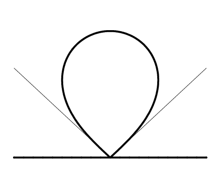
The simplest explicit solution to equation (6.2) known to us describes self-similar growth of a “fat slit” with degenerate base. The function
| (6.3) |
performs a conformal map from the exterior in ℍ of the curve , or, in polar coordinates,
| (6.4) |
to the upper half plane. This curve is shown in Fig. 6. In this case , , . The inverse map has the form
| (6.5) |
One can check that it does solve equation (6.2). More results on explicit solutions to Laplacian growth of fat slits will be published elsewhere.
7 Concluding remarks
We have constructed a parametric family of conformal maps of the upper half plane which is related to the dKP hierarchy with real “times” in the same way as conformal maps of the unit disk onto compact domains in the plane with smooth boundary are related to the dToda hierarchy with complex conjugate “times” , . Like in the dToda case, the deformations of domains (“fat slits”) in the upper half plane induced by dKP flows have a physical interpretation as Laplacian growth with certain type of sources or sinks at infinity. At the same time, our construction extends the well known connection between the dKP hierarchy and conformal maps of slit domains. In all cases, the conformal map plays the role of the Lax function.
However, a limiting procedure from fat slits to usual slits is singular and is not easy to trace on the level of the Lax equations. We hope that a better understanding of this limit will further clarify the geometric meaning of solutions to equations of the dKP hierarchy. We also expect that yet more general solutions can be obtained by the same method applied to the case of a background charge distributed in the upper half plane with a non-uniform density, in accordance with a similar construction given in [23].
The solutions discussed in this paper have a nice geometric meaning but it seems to be very hard to express them analytically in a closed form. In this respect the situation is less favourable than in the dToda case, where some simple explicit solutions for conformal maps as functions of a finite number of nonzero harmonic moments (corresponding, for example, to a parametric family of ellipses) are available. It is clear that in our case the situation when only a finite number of the moments are nonzero can not be realized because the local behavior of their generating function near the points , (which can be found from the integral representation (3.4)) shows that they are branch points of this function. This suggests that the corresponding solutions may be similar to the multi-cut solutions to Laplacian growth discussed recently in [24].
8 Appendices
Appendix A
Here we give some details of the derivation of the formula (3.11) for the time derivative of the function :
| (8.1) |
Here is the velocity of the normal displacement of the boundary at the point . Let be any parametrization of the contour such that is a steadily increasing function of the arc length, then it is a simple kinematical fact that
| (8.2) |
where is the line element along the contour. According to our convention, is positive when the contour, in a neighborhood of the point , moves to the right of the increasing direction.
Appendix B
In this Appendix we outline the proof of the following proposition.
-
Proposition 1. Let be a compact domain bounded by a closed piecewise analytic contour in the plane with a finite number of corner points. Consider the function defined by the Cauchy-type integral
(8.3) where is a bounded real-valued piecewise continuous function on such that
(8.4) and assume that for all . Then .
One can try to prove this statement by means of the following elementary argument. Let be the unit tangential vector to the curve at the point represented as a complex number. If for all , then the properties of Cauchy-type integrals imply that is the boundary value of a holomorphic function in vanishing at infinity. In fact is given by the same integral (8.3), where . Condition (8.4) tells us that the zero at infinity is of at least second order. Let be the conformal map from onto the unit disk such that and is real positive. By the well known property of conformal maps we have
along the curve . Therefore,
| (8.5) |
and we thus see that
is the boundary value of the holomorphic function . Since in , the function
is holomorphic there with the purely imaginary boundary value
Then the real part of this function is harmonic and bounded in and is equal to on the boundary. By uniqueness of a solution to the Dirichlet boundary value problem, must be equal to identically. Therefore, takes purely imaginary values everywhere in and so is a constant. By virtute of condition (8.4) this constant must be which means that .
However, this argument is directly applicable only for purely analytic contours for which all singularities and zeros of the function lie strictly inside it. For contours with corners, the corner points are singular points of the conformal map . Some more work is required to make the above argument rigorous. Below we present another proof of Proposition 1, which makes use of some non-trivial facts about boundary values of analytic functions and actually works in a much more general setting than just a finite number of corner points11 1 I thank D.Khavinson who suggested this proof and explained it to me.. It takes advantage of translating the proposition to a statement about analytic functions in the unit disk.
Sketch of proof of Proposition 1.
If defined by (8.3) is identically in , then it is analytic in , is near infinity (because of (8.4)) and has the boundary value almost everywhere on . (In our situation “almost everywhere” means everywhere except a finite number of points.) It is known [16, chapter III] that belongs to the Smirnov class .
Let be the conformal map from the unit disk onto such that and as with real . (The function is inverse to introduced above.) Set . Since
it follows from the above that is analytic in the unit disk with the boundary value
| (8.6) |
almost everywhere on the unit circle and has zero of at least second order at . Clearly, the function is analytic in the unit disk because the second order pole of at is canceled by the zero of . Furthermore, according to the Keldysh-Lavrentiev theorem [17, chapter 10], belongs to the Hardy class . But then the function belongs to the same Hardy class and takes purely imaginary boundary values
almost everywhere on the unit circle. The characteristic property of functions from the class is that they can be represented by the Poisson integral of their boundary values with real positive Poisson kernel (see [16, chapter II, ] or Theorem 3.9 in [17]). This means that must be purely imaginary everywhere inside the unit disk and hence must be a constant. Since , the constant is , so vanishes identically and .
The proof extends word for word to a more general case when is an integrable function with respect to (not necessarily bounded) and the boundary of is a rectifiable Jordan curve. It is crucial that the differential is real valued on the boundary. If one dropped that assumption, the statement is false. Moreover, functions from the class can have real boundary values in domains with cusps (see an example in [25]).
Acknowledgments
The author thanks D.Khavinson, I.Krichever, M.Mineev-Weinstein, T.Takebe, D.Vasiliev and P.Wiegmann for discussions and D.Khavinson for reading the manuscript. He is also grateful to organizers of the workshops “Laplacian growth and related topics” (CRM, Montreal, August 2008) and “Geometry and integrability in mathematical physics” (CIRM, Luminy, September 2008), where these results were reported. This work was supported in part by RFBR grant 08-02-00287, by grant for support of scientific schools NSh-3035.2008.2 and by the ANR project GIMP No. ANR-05-BLAN-0029-01.
References
- [1]
J. Gibbons and S. Tsarev, Reductions of
the Benney equations, Phys. Lett. A211 (1996) 19-24;
J. Gibbons and S. Tsarev, Conformal maps and reductions of the Benney equations, Phys. Lett. A258 (1999) 263-271. - [2] P. Wiegmann and A. Zabrodin, Conformal maps and integrable hierarchies, Commun. Math. Phys. 213 (2000) 523-538.
- [3]
I. Krichever, The -function of the
universal Whitham hierarchy, matrix models and topological field
theories, Comm. Pure Appl. Math. 47 (1994) 437-475,
e-print archive: hep-th/9205110;
I. Krichever, Funct. Anal Appl. 22 (1989) 200-213;
I. Krichever, The dispersionless Lax equations and topological minimal models, Commun. Math. Phys. 143 (1991) 415-429. - [4]
K. Takasaki and T. Takebe,
Integrable hierarchies and dispersionless limit, Rev. Math.
Phys. 7 (1995) 743-808;
K. Takasaki and T. Takebe, SDiff(2) Toda equation – hierarchy, tau function and symmetries, Lett. Math. Phys. 23 (1991) 205-214. - [5] M. Mineev-Weinstein, P. Wiegmann and A. Zabrodin, Integrable structure of interface dynamics, Phys. Rev. Lett. 84 (2000) 5106-5109, e-print archive: nlin.SI/0001007.
- [6] I. Krichever, M. Mineev-Weinstein, P. Wiegmann and A. Zabrodin, Laplacian growth and Whitham equations of soliton theory, Physica D 198 (2004) 1-28, e-print archive: nlin.SI/0311005.
- [7] A. Zabrodin, Growth processes related to the dispersionless Lax equations, Physica D235 (2007) 101-108, e-print archive: math-ph/0609023.
- [8] A comprehensive list of relevant papers published prior to 1998 can be found in: K. A. Gillow and S. D. Howison, A bibliography of free and moving boundary problems for Hele-Shaw and Stokes flow, http://www.maths.ox.ac.uk/ howison/Hele-Shaw/
- [9] B. Gustafsson, A. Vasil’ev, Conformal and Potential Analysis in Hele-Shaw Cells, Birkhäuser Verlag, 2006.
- [10] L. Yu and J. Gibbons, The initial value problem for reductions of the Benney equations, Inverse Problems, 16 (2000) 605-618.
- [11]
M. Manas, L. Martinez Alonso and E. Medina, Reductions and
hodograph solutions of the dispersionless KP hierarchy, J. Phys.
A.: Math. Gen., 35 (2002) 401-417;
M. Manas, -functions, reductions and hodograph solutions of the -th dispersionless modified KP and Dym hierarchies, J. Phys. A.: Math. Gen., 37 (2004) 11191-11221. - [12] I. Kostov, I. Krichever, M. Mineev-Weinstein, P. Wiegmann and A. Zabrodin, -function for analytic curves, in: Random Matrix Models and Their Applications, Math. Sci. Res. Inst. Publ. vol. 40, Cambridge University Press, pp. 285-299, e-print archive: hep-th/0005259.
- [13] A. Marshakov, P. Wiegmann and A. Zabrodin, Integrable Structure of the Dirichlet Boundary Problem in Two Dimensions, Commun. Math. Phys. 227 (2002) 131-153.
- [14] I. Krichever, A. Marshakov and A. Zabrodin, Integrable Structure of the Dirichlet Boundary Problem in Multiply-Connected Domains, Commun. Math. Phys. 259 (2005) 1-44.
- [15] J. Hadamard, Mém. présentés par divers savants à l’Acad. sci., 33 (1908).
- [16] I. I. Privalov, Randeigenschaften Analytischer Funktionen, Deutscher Verlag Wissenschaften, East Berlin, 1956 (translated from the second Russian edition I. I. Privalov, Granichnie svoistva analiticheskih funkciy, Gostehizdat, Moscow, Leningrad, 1950).
- [17] P. Duren, Theory of spaces, Academic Press, New York, 1970.
- [18] J. Akeroyd, D. Khavinson and H. Shapiro, Remarks concerning cyclic vectors in Hardy and Bergman spaces, Michigan Math. J. 38 (1991) 191-205.
- [19] J. R. King, A. A. Lacey and J. L. Vazquez, Persistence of corners in free boundaries in Hele-Shaw flow, Euro. J. Appl. Math. 6 (1995) 455-490.
- [20] P. J. Davis, The Schwarz function and its applications, The Carus Math. Monographs, No. 17, The Math. Assotiation of America, Buffalo, N.Y., 1974.
- [21] A. Orlov and E. Shulman, Additional symmetries for integrable equations and conformal algebra representation, Lett. Math. Phys. 12 (1986) 171-179.
- [22] B. Shraiman and D. Bensimon, Singularities in nonlocal interface dynamics, Phys. Rev. A30 (1984) 2840-2842.
- [23] A. Zabrodin, Dispersionless limit of Hirota equations in some problems of complex analysis, Theor. and Math. Phys. 129 (2001) 239-257.
- [24] Ar. Abanov, M.Mineev-Weinstein and A.Zabrodin, Multi-cut solutions to Laplacian growth, submitted to Physica D.
- [25] D. Khavinson, Remarks concerning boundary properties of analytic functions of -classes, Indiana Univ. Math. J. 31 (1982) 779-787.