Analytical Framework for Optimizing Weighted Average Download Time in Peer-to-Peer NetworksThanks: 

Fig. 2 shows a hierarchical P2P network with 4 peers, in which peer $i$ is in level $i$. Note that in this example, each peer downloads from all peers in the lower levels and uploads to all peers in the higher levels. However, by definition, peers are not required to download from all peers in the lower levels or upload to/from? all peers in the higher levels. For example, the network shown in Fig. 2 will still be a hierarchical P2P network if the edge $1\rightarrow 4$ vanishes. However, peers are not allowed to download from any peer in a higher level or upload to/from? any peer in a lower level. Also peers in the same level cannot download or upload to each other.

Proof:(by contraposition) Suppose there is a directed cycle $A_{1}\rightarrow A_{2}\rightarrow\cdots\rightarrow A_{n}\rightarrow A_{1}$, then some $A_{i}\rightarrow A_{i+1}$ or $A_{n}\rightarrow A_{1}$ violates the requirement that peers in a hierarchical P2P network cannot upload to a peer in a lower level. Therefore, the network containing the directed cycle cannot be a hierarchical P2P network. Q.E.D.

Proof:(by contraposition) Suppose a P2P network is not hierarchical, i.e., there exits a node $A$ in level $m$ and a node $B$ in level $n$ such that $m\geq n$ and $A\rightarrow B$. Let $S\rightarrow A_{1}\rightarrow\cdots\rightarrow A_{m-1}\rightarrow A$ be the longest directed acyclic path from $S$ to $A$ and $S\rightarrow B_{1}\rightarrow\cdots\rightarrow B_{n-1}\rightarrow B$ be the longest directed acyclic path from $S$ to $B$. Since $S\rightarrow A_{1}\rightarrow\cdots\rightarrow A_{m-1}\rightarrow A\rightarrow B$ is a directed path from $S$ to $B$ with length $m+1>n$, this path must contain a directed cycle, and hence, the P2P network is not a directed acyclic graph. Therefore, a directed acyclic P2P network is a hierarchical P2P network. Q.E.D.

It is a direct consequence of Lemma 1 and Lemma 2.

Fig. 3 shows a strictly hierarchical P2P network with 3 levels. In a strictly hierarchical P2P network, peers in level $K$ work together as a virtual server and upload to peers in level $K+1$. In Fig. 3, peer 1 and 2 form the virtual server in level $1$, denoted as $S_{1}$. Peer 3, 4 and 5 form the virtual server in level $2$, denoted as $S_{2}$. Since all transmission flows are between two consecutive levels, peer selection algorithms and chunk selection algorithms can be locally designed level by level.

The relationships among the P2P network, the hierarchical P2P network and the strictly hierarchical P2P network are concluded in Fig. 4.

A P2P overlay network is divisible if peers can be divided into sub-peers, and it is indivisible if peers cannot be divided. The division of peers can be performed at the application layer [4] [23]. Even for indivisible P2P network, peers can be conceptually divided into virtual sub-peers for theoretical analysis. A simple example of peer division is given in Fig. 5. Fig. 5(a) shows the original P2P network and Fig. 5(b) shows the network of sub-peers after the division of peer 1 into sub-peer $1A$ and sub-peer $1B$.

A peer division is equivalent if the transmission rates from the server to each peer and from each peer to each other peer are invariant. The network of sub-peers is equivalent to the original P2P network if the peer division is equivalent. The peer division in Fig. 5 is equivalent if $r_{s\rightarrow 1}=r_{s\rightarrow 1A}$, $r_{1\rightarrow 2}=r_{1A\rightarrow 2}$ and $r_{3\rightarrow 1}=r_{3\rightarrow 1B}$.

Proof of Theorem 2: In order to prove the theorem, it suffices to construct a strictly hierarchical network of sub-peers which is equivalent to the original P2P network. For any P2P network with $N$ peers and $K$ levels, denote the server $S$ as node $0$ and the peers as node $1,2,\cdots,N$. Let

and so $|K_{i}|\leq K$ is the cardinality of $K_{i}$. Divide peer $i$ into $|K_{i}|$ sub-peers, which are denoted as sub-peer $(i,k)$ for $k\in K_{i}$. The sub-peer $(i,k)$ is the part of peer $i$ in level $k$. In the network of sub-peers, there is an edge from the server $S$ to sub-peer $(i,1)$ if and only if $S\rightarrow i$ in the original network. We assign the transmission rate $r_{s\rightarrow(i,1)}=r_{s\rightarrow i}$. There is an edge from sub-peer $(i,k)$ to sub-peer $(j,k+1)$ if and only if there exits a directed acyclic path with length $k+1$ such that $S\rightarrow\cdots\rightarrow i\rightarrow j$ in the original P2P network. We assign the transmission rates level by level with

where $r_{(i,k)}$ is the total download rate of the sub-peer $(i,k)$, $r_{i\rightarrow j}$ is the transmission rate from peer $i$ to peer $j$ in the original P2P network, $r_{i\rightarrow j}^{k}$ is the unassigned transmission rate from peer $i$ to peer $j$ until level $k$ in the network of sub-peers, and $r_{(i,k)\rightarrow(j,k+1)}$ is the transmission rate from $(i,k)$ to $(j,k+1)$. This division for the network in Fig.5(a) is shown in Fig. 6(a).

Since $|K_{i}|\leq K$ for all $i$, the constructed network of sub-peers has at most $K$ levels. There are at most $N$ sub-peers in each level because each level contains at most one sub-peer of any peer. It is also easy to check that the constructed network of sub-peers is strictly hierarchical.

In order to prove that the network of sub-peers is equivalent to the original P2P network, we need to show that

If $i=0$, i.e., node $i$ the server $S$, then

If $i\neq 0$, suppose for all $k\leq K$,

then

and so

which is infeasible. Hence, there always exists some $m\leq K$ such that

then $r_{i\rightarrow j}^{k}=0$ for $k\geq m$, $r_{(i,k-1)\rightarrow(j,k)}=0$ for $k>m$, and hence

Finally, we need to show that the assigned transmission rates in the network of sub-peers are feasible, i.e., the download rate of each sub-peer is greater than or equal to it upload rate. Plugging $j=N$ into (4),

and so

Q.E.D.

If edges with zero transmission rate and sub-peers with zero download bandwidth and zero upload bandwidth are allowed, divide peer $i$ into $K$ sub-peers, which are denoted as sub-peer $(i,k)$ for $k=1,\cdots,K$. The sub-peer $(i,k)$ is the part of peer $i$ in level $k$. There is an edge from the server $S$ to sub-peer $(i,1)$ for all $i$. There is an edge from sub-peer $(i,k)$ to sub-peer $(j,k+1)$ for all $i\neq j$. The network of sub-peers after this division is also strictly hierarchical, and keeps all the transmission paths in the original network. This peer division for the P2P network in Fig. 5(a) is shown in Fig. 6(b), in which the dotted border sub-peers have zero download bandwidth and zero upload bandwidth, and the dotted edges have zero transmission rate. By Theorem 2, there exits a transmission rate assignment such that the network of sub-peers after this peer division is equivalent to the original P2P network. Hence, minimizing the WADT for strictly hierarchical networks of sub-peers is equivalent to minimizing the WADT for P2P networks.

In a very large P2P network with $N$ peers, the length of the longest directed acyclic path $K=\max_{i}|K_{i}|$ is usually much less than $N$. Denote $d_{i,j},u_{i,j},r_{i,j}$ as the download bandwidth, upload bandwidth and the download rate of the part of peer $i$ in level $j$, where $d_{i,j}\geq u_{i,j}$ and $d_{i,j}\geq r_{i,j}$. The sub-peers in level $j$ work together as a virtual server to upload to the sub-peers in level $j+1$. Denote $S_{j}$ as the upload bandwidth of the virtual server in level $j$, $1\leq j\leq K$, and so $S_{j}=\sum_{i=1}^{N}\min(u_{i,j},r_{i,j})$. Let $S_{0}=S$.

Proof: Suppose $d_{i,j},u_{i,j},r_{i,j}$ determine an optimal strictly hierarchical network of sub-peers which connects the server and the peers, and achieves the minimum WADT. It is clear that $\tilde{d}_{i,j},\tilde{u}_{i,j},\tilde{r}_{i,j}$ is also an optimal strictly hierarchical network of sub-peers which has $\tilde{r}_{i,j}\geq\tilde{u}_{i,j}$ for any $1\leq i\leq N$, $1\leq j\leq K-1$, where

The theorem is immediately proved. Q.E.D.

Theorem 2 demonstrates that minimizing the WADT for P2P networks with $N$ peers and $K$ levels is equivalent to minimizing the WADT for strictly hierarchical networks of sub-peers with $K$ levels, each of which contains $N$ sub-peers. $K\ll N$ for large P2P networks. Recall that the bandwidth of the server is $S=S_{0}$. The download bandwidth and upload bandwidth of peer $i$ are $d_{i}$ and $u_{i}$ respectively, where $d_{i}\geq u_{i}$. $S_{j}$ is the bandwidth of the virtual server in level $j$, $1\leq j\leq K$. $d_{i,j},u_{i,j},r_{i,j}$ are the download bandwidth, the upload bandwidth and the download rate of the part of peer $i$ in level $j$.

The constraints on the download bandwidths and upload bandwidths are $d_{i,j}\geq u_{i,j}$ for any $1\leq i\leq N$ and $1\leq j\leq K$, $\sum_{j=1}^{K}d_{i,j}=d_{i}$ and $\sum_{j=1}^{K}u_{i,j}=u_{i}$ for any $1\leq i\leq N$. The constraints on the download rates are $r_{i,j}\leq d_{i,j}$ for any $1\leq i\leq N$ and $1\leq j\leq K$. Lemma 6 shows that any optimal strictly hierarchical network of sub-peers has $r_{i,j}\geq u_{i,j}$ for any $1\leq i\leq N$ and $1\leq j\leq K-1$. $\sum_{j=1}^{K}r_{i,j}=r_{i}$ is the total download rate for peer $i$. Corollary 1 demonstrates that the bandwidth of the virtual server in level $j$ is $S_{j}=\sum_{i=1}^{N}u_{i,j}$ for $j=1,\cdots,K-1$. One has $S_{j-1}\geq\sum_{i=1}^{N}r_{i,j}$ since the virtual server in Level $j-1$ uploads content to the sub-peers in Level $j$.

All the constraints are linear and the objective function, $\sum_{i=1}^{N}w_{i}/r_{i}$, is a convex function. Therefore, the problem of minimizing the WADT is a convex optimization program, which can be solved by convex optimization solvers such as the interior-point method. The complexity of the interior-point method to solve this problem is $o(\sqrt{K^{3}N^{3}})$ [25]. The solution to the convex optimization program provides the topology of the optimal P2P network which achieves the minimum WADT, however, the number of the peers is usually very large for most P2P applications and so the complexity for solving the convex program is too high. Fortunately, this convex program has an analytical achievable upper bound which is very tight to the optimal solution and its complexity is linear to the number of the peers in a P2P network.

Theorem 1 shows that any hierarchical P2P network contains no directed cycle and vice versa. Constructing a hierarchical P2P network shown in Fig.7 provides an achievable upper bound for the minimum WADT. Assume that $S\gg\max_{i}(u_{i})$, which is always true practically. Without loss of generality, assume $u_{1}\geq u_{2}\geq\cdots\geq u_{N}$. Partition the server into two parts $S^{(1)}=\max_{i}(u_{i})=u_{1}$ and $S^{(2)}=S-\max_{i}(u_{i})=S-u_{1}$. The first part $S^{(1)}$ can serve all the peers with $r_{i}^{(1)}=u_{i}$. The second part $S^{(2)}$ can then freely serve for the peers only with the constraints $d_{i}\geq r_{i}^{(1)}+r_{i}^{(2)}\geq u_{i}$ and $S^{(2)}\geq\sum_{i}^{N}r_{i}^{(2)}$. Thus, the upper bound is the solution to the optimization problem

The Karush-Kuhn-Tucker conditions for the optimal solution are

Combining the the Karush-Kuhn-Tucker conditions and the constraints in the problem, we obtain the upper bound which is $\sum_{i=1}^{N}w_{i}/r_{i}$ with

where $R$ is chosen appropriately such that $\sum_{i=1}^{N}(r_{i}-u_{i})=S-\max_{i}(u_{i})$.

This upper bound is almost optimal. Consider the following lower bound which is very close to the upper bound. Since $S\geq\sum_{i=1}^{N}(r_{i}-u_{i})$ is a relaxed constraint, an lower bound is the solution to the optimization problem

Note that this optimization problem (19) differs from the problem (17) only by replacing $S$ with $S-\max_{i}(u_{i})$. Thus, the lower bound is $\sum_{i=1}^{N}w_{i}/r_{i}$ with

where $R$ is chosen appropriately such that $\sum_{i=1}^{N}(r_{i}-u_{i})=S$.

Since $S\gg\max(u_{i})$, one has $S\simeq S-\max_{i}(u_{i})$. The upper bound and the lower bound are almost the same. Therefore, both of these two bounds are very tight, and the upper bound is almost an analytical solution to minimizing the WADT. Hence, it is sufficient to build a hierarchical P2P network to achieve the minimum WADT.

Compared with building networks of sub-peers and hierarchical P2P networks, it is more practical to build a strictly hierarchical P2P network. First, in a strictly hierarchical P2P network, peers do not need to be decomposed into sub-peers. Thus, it can have a much simpler protocol in network layer than a network of sub-peers. Second, in a strictly hierarchical P2P network, each level usually contains only tens or hundreds of peers. Therefore, one can locally design peer selection algorithms and chunk selection algorithms level by level, which only depend on a small collection of peers in the P2P network. The locally designed peer and chunk selection algorithm might be much simpler than the network coding strategy and other global designed peer and chunk selection algorithms. The following theorem shows that there exists a strictly hierarchical network of sub-peers which achieves the upper bound in the previous subsection, and is very close to a strictly hierarchical P2P network.

Proof: Equation (18) gives $r_{i}$, $i=1,\cdots,N$, for the hierarchical P2P network which achieves the upper bound. Convert the hierarchical P2P network to multiple optimal strictly hierarchical networks of sub-peers by the following algorithm.

This algorithm indicates that at most $K-1$ peers need to be divided into 2 sub-peers and each level of the constructed network of sub-peers contains at most 2 sub-peers. Since there are multiple choices in step (2), this algorithm provides multiple strictly hierarchical networks of sub-peers which are very close to a strictly hierarchical P2P network. Q.E.D.

Another practical solution is to solve the problem of minimizing the WADT directly for strictly hierarchical P2P networks. This problem can be formulated as a 0-1 convex optimization. The complexity to solve a 0-1 convex optimization problem is exponential to the problem size.

Fortunately, this problem has an analytical suboptimal solution. Suppose there are $N$ peers and $K$ levels in a strictly hierarchical P2P network and the level location of each peer is already given. Then the global optimization problem can be decomposed into $K$ local optimization problem and all of them have an analytical “Water Filling” solution.

In particular, suppose the bandwidth of the server is $S=S_{0}$. The download bandwidth, upload bandwidth and the allocated download rate of Peer $i$ are $d_{i}$, $u_{i}$ and $r_{i}$ respectively. $S_{j}$, the bandwidth of the virtual server in Level $j$, is equal to the summation of the upload bandwidths of the peers in Level $j$. If $S_{j}$ is greater or equal to the summation of the upload bandwidth of all peers in level $j+1$, then one has $d_{i}\geq r_{i}\geq u_{i}$ and $S_{j+1}=\sum_{\textrm{Peer }i\textrm{ in level }j}u_{i}$. If $S_{j}$ is less than the summation of the upload bandwidth of all peers in level $j+1$, one has $0\leq r_{i}\leq u_{i}$ and $S_{j+1}=S_{j}=\sum_{\textrm{Peer }i\textrm{ in level }j}r_{i}$. Therefore, no matter how to allocate download rates to peers in each level, the bandwidth of the virtual server in each level is fixed as long as the level positions of peers are fixed. Thus, the global minimum weighted average transmission rate problem can be decomposed to $K$ local optimization problem. Each of them has a fixed server bandwidth and fixed number of peers in the level. Thus, if the virtual server $S_{j}$ is greater or equal to the summation of the upload bandwidth of all peers in level $j+1$, then the local optimization problem is

where $N_{j+1}$ is the number of peers in level $j+1$, for $j=0,\cdots,K-1$.

By the Karush-Kuhn-Tucker conditions, the optimal solution is

where $R$ is chosen appropriately such that $\sum_{i=1}^{N_{j+1}}r_{i}=S_{j}$.

If the virtual server $S_{j}$ for level $j+1$ is less than the summation of the upload bandwidth of all peers in level $j+1$, then the local optimization problem is

where $N_{j+1}$ is the number of peers in level $j+1$, for $j=0,\cdots,K-1$.

By the Karush-Kuhn-Tucker conditions, the optimal solution is

where $R$ is chosen appropriately such that $\sum_{i=1}^{N_{j+1}}r_{i}=S_{j}$.

In this small simulation, the bandwidth of the server is 10 and the number of the peers in the network is $N=100$. The download bandwidths $d_{i}$, $i=1,\cdots,100$, are i.i.d. with uniform distribution over $[0.01,1.99]$, i.e., $\beta=10^{-2}$. For each peer $i$, the upload bandwidth is uniformly distributed over $[0.1d_{i},d_{i}]$, i.e., $\alpha=0.1$. The weights for all the peers are equal and normalized to be $1/N=1/100$, and so $\sum_{i}w_{i}=1$. Thus, the WADT is $\sum_{i}w_{i}/r_{i}$. We will compare 7 methods in this experiment. They are

• •

  1. Optimal solution to the convex optimization program with level $K=30$. The convex program solver is CVX [26].

• •

  2. The upper bound (17) by constructing a hierarchical P2P network.

• •

  3. The lower bound (19) by relaxing the constraints.

• •

  4. The suboptimal solution to the 0-1 convex optimization problem for strictly hierarchical P2P networks. The number of the levels are set to be $K=30$ and we randomly put around $N/K$ peers in each level.

• •

  5. The suboptimal solution to the 0-1 convex optimization problem for strictly hierarchical P2P networks. We convert the upper-bound-achieving hierarchical P2P network (Method 2) to a network of sub-peers by Algorithm 1. The peers are placed into levels according to the constructed network of sub-peers, which is very close to a strictly hierarchical P2P network.

• •

  6 This is a trivial upper bound such that the rate of each peer is the same as the upload bandwidth.

• •

  7 This is a trivial lower bound such that the rate of each peer is the same as the download bandwidth.

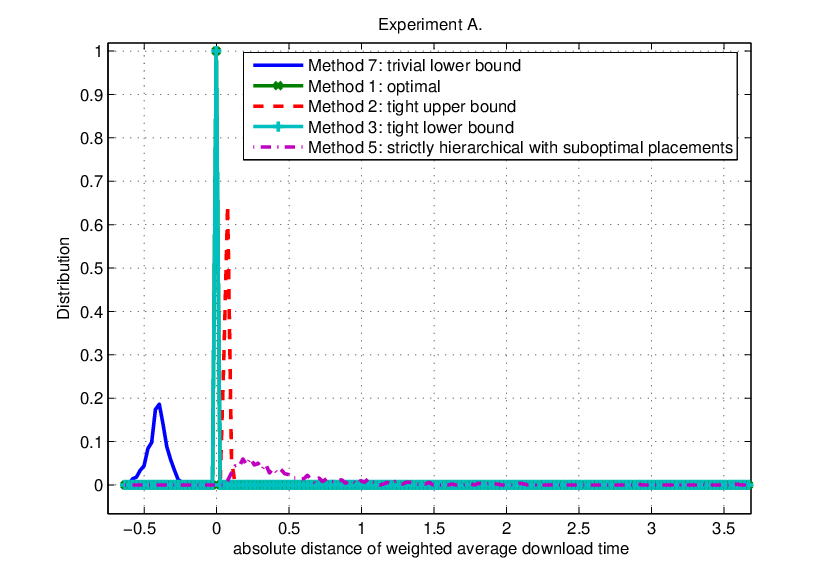
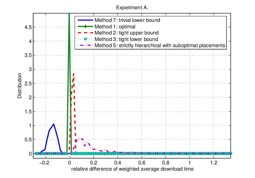
The distribution of the weighted average download times of 500 experiments are shown in Fig. 8. The distribution of the difference and the relative difference between Method 3 and other methods are shown in Fig. 9 and Fig. 10. The weighted average download times of Method 1 is concentrated in the range of $[1.7,4.1]$ with mean value 2.877. Method 2 and Method 3 provide the upper bound and lower bound for the minimum WADT. Fig. 8, 9, and 10 show that these two bounds are very tight. In this case, the lower bound is almost always the same as the optimal solution since the distribution curves of Method 1 and Method 3 perfectly match. The distribution curve of Method 2 is slightly different from that of Method 1, which means that the upper bound is only slightly larger than the optimal solution for most of the experiments. In this simulation, the bandwidth of the server is 10, which is not much larger than the maximum of the upload bandwidths. That is why the upper bound is still slightly different from the optimal solution. The distribution of Method 5 shows that in most of the experiments, the WADT of Method 5 is close to the optimal solution, however, it is sometimes much larger than the optimal solution. This is because the peer placement in Method 5 is usually very good but sometimes bad. Note that it is NP complete complex to find the best peer placement. In order to improve Method 5 without increasing the complexity, we need provide a better but still low-complex peer placement algorithm. The performance of Method 4 is much worse than the performance of Method 5 because the peer placement algorithm is Method 4 is much worse that in Method 5.

The bandwidth usage is the ratio of the total transmission rate and the total download bandwidth of all the peers in the network. For a fixed WADT, it is clear that the lower bandwidth usage the better. However, it is a trade off to decrease the bandwidth usage and to decrease the WADT, which is also verified in Fig. 11. Fig. 11 shows the distribution of the bandwidth usage of different methods. The distribution of Method 1, the optimal solution, is exactly the same as the distribution of Method 3, the lower bound. The bandwidth usage of Method 2, the upper bound, is slightly less than that of Method 1 and the bandwidth usage of Method 5 is slightly less than that of Method 2. It is verified that the method with smaller WADT always has higher bandwidth usage. The mean values of the weighted average download times and the bandwidth usage of different methods are listed in Table I.

For one typical experiment, the plots of the virtual server bandwidths versus the levels for different methods are shown in Fig. 12. For Method 1, the number of the levels $K$ is manually chosen. In this experiment,$K$ is 30. One can see that the bandwidths of the virtual servers from level 5 to level 30 are linearly decreasing to 0 for Method 1. The bandwidth of the virtual server generated by the last level is almost 0. In other words, all the upload bandwidths of the server and the peers are fully used. This is the reason why the performance of Method 3, the tight lower bound, is almost the same as that of Method 1. For Method 2, the number of the levels needed is automatically solved. It is 15 in this experiment.

In this simulation, the bandwidth of the server is 50 and there are 4000 peers in the network. The download bandwidths $d_{i}$, $i=1,\cdots,4000$, are i.i.d. with uniform distribution over $[0.01,1.99]$. The upload bandwidth $u_{i}$ is uniformly distributed over $[0.1d_{i},d_{i}]$. The weights for all the peers are equal and normalized to be $1/N=1/4000$, and so $\sum_{i}w_{i}=1$.

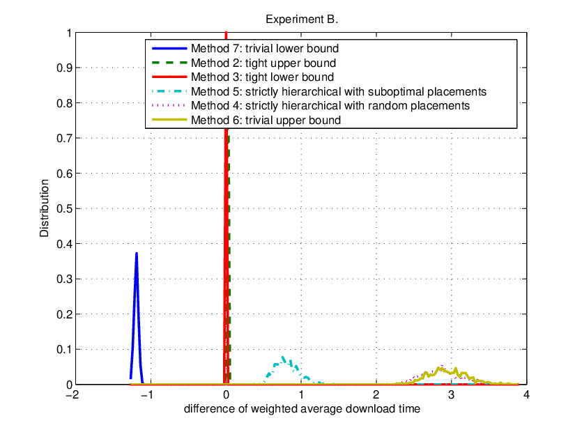
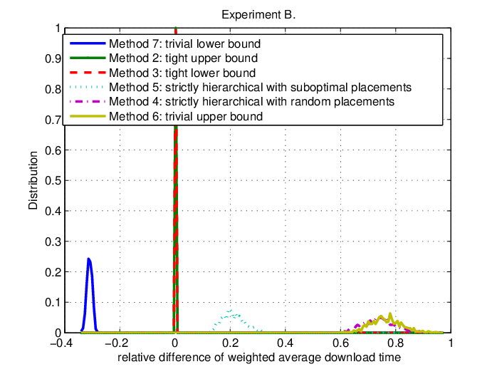
The distribution of the weighted average download times of 800 experiments are shown in Fig. 13. The distribution of the difference and the relative difference between Method 3 and other methods are shown in Fig. 14 and Fig. 15. These figures show that the lower bound and the upper bound provided by Method 3 and Method 2 are very close. The performance of Method 1 should be between these two bounds, although we don’t simulate Method 1 in this case. In this simulation, the bandwidth of the server is 50, which is much larger than the maximum of the upload bandwidths. That is why $S\simeq S-\max_{i}(u_{i})$ and the upper bound is almost the same as the lower bound. The performance of Method 5 is worse than that of Method 2 but still a lot better that of Method 6 and 7.

The bandwidth usages of these methods are shown in Fig. 16. The distribution of Method 2 is almost the same as the distribution of Method 3, which verifies the almost same performance of Method 2 and 3. The mean values of the weighted average download times and the bandwidth usage of different methods are listed in Table II. Combining the simulation results, the comparison of these 7 methods in different criteria are listed in Table III.