MZ-TH/08-32 Bare Action and Regularized Functional Integral of Asymptotically Safe Quantum Gravity
Abstract
Investigations of Quantum Einstein Gravity (QEG) based upon the effective average action employ a flow equation which does not contain any ultraviolet (UV) regulator. Its renormalization group trajectories emanating from a non-Gaussian fixed point define asymptotically safe quantum field theories. A priori these theories are, somewhat unusually, given in terms of their effective rather than bare action. In this paper we construct a functional integral representation of these theories. We fix a regularized measure and show that every trajectory of effective average actions, depending on an IR cutoff only, induces an associated trajectory of bare actions which depend on a UV cutoff. Together with the regularized measure these bare actions give rise to a functional integral which reproduces the prescribed effective action when the UV cutoff is removed. In this way we are able to reconstruct the underlying microscopic (“classical”) system and identify its fundamental degrees of freedom and interactions. The bare action of the Einstein-Hilbert truncation is computed and its flow is analyzed as an example. Various conceptual issues related to the completion of the asymptotic safety program are discussed.
1 Introduction
The problem of finding a fundamental quantum theory of gravity is still an exciting challenge which is pursued within a variety of approaches [1, 2, 3, 4]. In the context of the asymptotic safety program [5]-[28], for instance, a lot of efforts were devoted to establishing the existence of an ultraviolet fixed point at which Quantum Einstein Gravity (QEG) can be renormalized. Detailed calculations revealed that the renormalization group (RG) flow of the theory does indeed possess an appropriate non-Gaussian fixed point (NGFP) in all approximations which were investigated.
Formulated in terms of the gravitational average action as proposed in [6], the RG flow in question is that of the effective average action , henceforth abbreviated EAA [29],[34]. While similar in spirit to the idea of a Wilson-Kadanoff renormalization, it replaces the iterated coarse graining procedure by a direct mode cutoff at the infrared (IR) scale . More importantly, the EAA is a scale dependent version of the ordinary effective action, while a “genuine” Wilsonian action is a bare action, i.e. it is to be used under a regularized path integral. As a result, it depends on the ultraviolet (UV) cutoff ; its dependence on is governed by a RG equation which is different from that for .
In a sense, for different values of is a set of actions for the same system: the Green’s functions have to be computed from by a further functional integration over the low momentum modes, and this integration renders them independent of . By contrast, the EAA can be thought of as the standard effective action for a family of different systems: for any value of it equals the standard effective action of a model with the bare action where is the mode suppression term. The corresponding -point functions do depend on ; they provide an effective field theory description [35]-[47] of the physics at scale . These -point functions are simply the functional derivatives of , so their computation requires no further functional integration. (See [33, 28] for a disscussion of this point.)
In the EAA framework, a quantum field theory is fully defined once a complete RG trajectory has been constructed, that is, a solution of the functional RG equation (FRGE) for which is well defined for all . In particular it must be free from divergences in the IR () and the UV (). In asymptotically safe theories the latter condition is met by arranging the RG trajectory to hit the NGFP in the limit . Given a complete trajectory we have, in principle, complete knowledge of all properties of the quantum theory at hand. Its Green’s functions are the derivatives of and at they coincide with those of the standard effective action [29].
Because of these differences between the EAA and a genuine Wilson action, this way of constructing an asymptotically safe field theory does not by itself yield a regularized path integral over metrics whose “continuum limit” would be related to the RG trajectory in a straightforward way. In order to understand this important point let us recall how the EAA was employed in gravity up to now.
The starting point for the definition of the EAA and the derivation of its flow equation is a path integral over metrics, which is UV regularized in some way. This path integral is reformulated in a background field language, gauge fixed, augmented by source terms, and then a mode suppression term is added to . By definition, the EAA is essentially the Legendre transform of the resulting generating functional. Its FRGE is found by straightforwardly applying the scale derivative to this definition.
One of the salient features of this FRGE is that it continues to be well behaved in the ultraviolet even when the UV regulator originally built into the path integral is removed11 1 This requires an appropriate fall-off behavior of the coarse graining kernel, which we always assume in the following.. Roughly speaking the reason is that receives contributions only from modes with covariant momenta near (or below) . In fact, in all investigations which employed the gravitational EAA so far[6]-[26], the FRGE without an UV regulator (“-free FRGE”) has been used. For instance, the NGFP that has been discovered refers to the RG flow implied this “-free” equation.
The UV regularization being superfluous at the FRGE level has both advantages and disadvantages. Clearly, the major advantage is that it allows us to search for asymptotically safe theories directly at the effective level, without the additional burden of having to construct a regularized path integral and control its infinite cutoff limit.
Note that the question of whether or not a theory is asymptotically safe is decided by the properties of the effective - as opposed to the bare- action since the former is directly related to S-matrix elements, say. They are free from divergences if their generating functional is so, and this in turn is the case when is connected to a fixed point by a complete, everywhere regular RG trajectory . On the other hand, the relation between the -matrix elements and the bare action that would enter a regularized path integral is much more indirect. A priori we do not know which behavior of for corresponds to the absence of divergences in observable quantities and to a fixed point . In general the relationship between and will depend on how we regularize the path integral measure .
Working with the -free FRGE, the advantage is that all problems related to the path integral, its bare action and measure, can be sidestepped. The corresponding disadvantage is that even if we knew an exact, complete RG trajectory which would amount to a well defined quantum field theory, we would not have a path integral formulation of this theory at our disposal, and we could not even be sure that such a formulation actually exists.
Conceptually there is nothing wrong with that. For systems with finitely many degrees of freedom canonical quantization, path integral quantization and the quantization by a FRGE are equivalent but we cannot be sure that this equivalence will always hold true in quantum field theory. In principle the -free FRGE could yield a physically completely satisfactory quantum field theory, predictive and consistent, but has no path integral representation. However, in the following we shall argue that this is actually not what happens in QEG.
In fact, in this paper we are going to demonstrate that it is possible to “reconstruct” a regularized functional integral in such a way that it describes a fixed, prescribed asymptotically safe theory in the infinite cutoff limit. This path integral representation is not “canonically” given, however, as it requires an extra ingredient, namely an UV regularization scheme. Adopting a particularly convenient UV scheme we shall see that the information contained in is sufficient in order to determine the related bare action in the limit . We prescribe a trajectory and deduce from it how the bare coupling constants contained in must behave in the UV limit when the path integral (with the measure and action defined according to the special scheme adopted) is required to reproduce the prescribed trajectory.
Under conditions that we shall spell out precisely later on, one finds that for the bare action equals essentially at :
| (1.1) |
The -dependent “correction term” depends on the UV regularization scheme chosen and cannot be found from the flow equation. We are going to discuss its general properties and compute it explicitly for various examples, including the Einstein-Hilbert truncation of QEG.
Equation (1.1) is to be regarded a precise, regularized version of the “rule of thumb” which is quoted frequently, “”. In most applications of the EAA in particle and condensed matter physics the -contribution in (1.1) is completely unimportant and usually not considered explicitly. In fact, in a perturbatively renormalizable theory the only effect of the -term is to shift those (very few) bare couplings which are relevant at the Gaussian fixed point. In typical EAA applications one is not interested in their exact values (more precisely, the way how they diverge for ) since one anyhow wants to parameterize the RG trajectory by their renormalized counterparts, to be determined experimentally.
An example in which has been studied in detail is Liouville field theory [32]. There the exact values of the bare couplings are of some interest since, being “almost topological”, the RG effects in this theory are so weak that the running couplings change by only a finite amount during an infinitely long RG time. In asymptotically safe theories is important for an analogous reason. In fact, the RG trajectories of Liouville theory cross over from an UV to an IR fixed point so that, in a sense, this theory is asymptotically safe, too [32].
There are various motivations for trying to construct a path integral representation of QEG:
(i) The most important motivation, at least from a conceptual point of view, is probably the following. In our approach the primary definition of the quantum field theory is in terms of an EAA-trajectory with a UV fixed point. Its endpoint is the ordinary effective action , so we can easily compute all Green’s functions. However, what we have no easy access to is the microscopic (or “classical”) system whose standard quantization gives rise to this particular effective action. A functional integral representation of the asymptotically safe theory will allow the “reconstruction” of the microscopic degrees of freedom that we implicitly integrated out in solving the FRGE, as well as their fundamental interactions. The path integral provides us with their action, and from this action, by a kind of generalized Legendre transformation, we can reconstruct their Hamiltonian description. From this phase space formulation we can read off the classical system whose quantization (also by other methods, canonically say) leads to the given effective action. We expect this system to be rather complicated so that it cannot be guessed easily. This is why we start at the effective level where we know what to look for, namely a whose functional derivatives (-matrix elements) are such that observable quantities have no divergences on all momentum scales.
(ii) Another motivation is that many general properties of a quantum field theory are most easily analyzed in a path integral setting, the implementation of symmetries, the derivation of Ward identities or the incorporation of constraints, to mention just a few.
(iii) Many approximation schemes (perturbation theory, large-N expansion, etc.) are more naturally described in a path integral rather than a FRGE language. A standard way of doing perturbation theory is to compute, order by order, the counter terms to be included in to get finite physical results in the limit . Now, QEG is not renormalizable in perturbation theory and hence new counter terms with free coefficients must be introduced at each order. If, on the other hand, QEG is asymptotically safe, defined by a complete trajectory , this trajectory “knows” the correct UV completion of the perturbative calculation. But in order to extract this information from and make contact with the perturbative language of -counter terms we must convert the -trajectory to a -trajectory first.
(iv) As a last motivation we mention that ultimately we would like to understand how QEG relates to other approaches to quantum gravity, such as canonical quantization, loop quantum gravity [2, 3, 4] or Monte Carlo simulations [51]-[54], in which the bare action often plays a central role. In the Monte Carlo simulations of the Regge and dynamical triangulations formulation, for instance, the starting point is a regularized path integral involving some discrete version of , and in order to take the continuum limit one must fine tune the bare parameters in in a suitable way. If one is interested in the asymptotic scaling, for instance, and wants to compare the analytic QEG predictions to the way the continuum is approached in the simulations, one should convert the -trajectory to a -trajectory first. Note that the map from to , i.e. the associated functional depends explicitly on how precisely the path integral is discretized; each alternative formulation of QEG has its own !
The remaining sections of this paper are organized as follows. In Section 2 we discuss the EAA technology needed later on, the FRGE with a UV cutoff, the relation of its solutions to those of the -free FRGE, and we explain why the EAA approach, despite its obvious similarity with the Kadanoff-Wilson momentum shell integration is not completely equivalent to it. Then, in Section 3 we demonstrate that every -trajectory induces a trajectory of bare actions and show how it can be found. Section 4 illustrates the method by means of a simple toy model which, however, is of physical interest in its own right: the running cosmological constant induced by a scalar matter field. Section 5 is devoted to QEG. Within the Einstein-Hilbert truncation we compute and analyze the map from the effective to the bare couplings in explicit form. In Section 6 we give a brief summary and discuss various general conceptual issues related to the Asymptotic Safety program in QEG.
2 Effective Average Action with UV cutoff
In this section we describe how the functional integral underlying the definition of the effective average action can be made well defined. We regularize it by introducing an UV cutoff and then derive, in a completely well defined way, the corresponding EAA and its flow equation in presence of . Many different regularization schemes are conceiveable here. For concreteness we use a kind of “finite mode regularization” which is ideally suited for implementing the “background independence” mandatory in QEG.
2.1 The EAA framework
In this section, for notational simplicity, we consider a single scalar field on flat space. The generalization to more complicated theories can be achieved by obvious notational changes.
Let be a real scalar field on a flat -dimensional Euclidean spacetime. In order to discretize momentum space we compactify spacetime to a -torus. As a result, the eigenfunctions of the Laplacian are plane waves with discrete momenta and eigenvalues . Given a UV cutoff scale , there are only finitely many eigenfunctions with . We regularize the path integral in the UV by restricting the integration to those modes.
As is standard in the EAA construction [29, 33], the IR modes with are suppressed in the path integral by the factor where the functional provides a kind of momentum dependent mass term:
| (2.1) |
Now we define a UV-regulated analogue of the standard functional :
| (2.2) |
The notation in eq.(2.2) is symbolic. In fact, its RHS involves only finitely many integrations and is not a genuine functional integral. The field and the source in (2.2) are “coarse grained” in the sense that they have an expansion
| (2.3) |
and similar for . Likewise, the measure stands for an integration over the Fourier coefficients with below :
| (2.4) |
The arbitrary mass parameter was introduced in order to give the canonical dimension zero to (2.4). Even though in eq. (2.2) and similar formulas we keep using the familiar (functional) notation, it is to be kept in mind that and stand for a finite set of variables.
In (2.2) the bare action is allowed to depend on the UV cutoff. Ultimately we would like to fix this -dependence in such a way that, for every finite and , the path integral has a well defined limit for .
Denoting the Legendre transform of with respect to by the EAA is defined as [29]
| (2.5) |
Here is the expectation value field obtained by differentiating . In the usual notation,
| (2.6) |
If this relation can be inverted in the form we have
| (2.7) |
and
| (2.8) |
By following the usual steps [29] it is straightforward to show that the definition (2.5) implies the following exact FRGE for :
| (2.9) |
Here, denotes the trace restricted to the subspace spanned by the eigenfunctions of with eigenvalues smaller than :
| (2.10) |
As it is customary, denotes the Hessian of , interpreted as an operator constructed from and the conjugate position variable .
2.2 EAA vs. momentum shell integration
| (a) | (b) |
|---|---|
 |
 |
The key feature of the EAA is the mode suppression term which gives a mass of order to the field modes with momenta . How this happens precisely is controlled by the function . The details of this function are irrelevant to a large extent; we only require that is a monotonic function of which interpolates between and , whereby the transition between the two regimes takes place near . An example sketched in Fig.1a. Its scale derivative has a peak near , a very rapid (exponential) decay for , and for a plateau on which is an approximately constant function of . We shall refer to the and regime of , respectively, as the “exponential tail” and the “low- continuum”.
Most of the somewhat unexpected features of the EAA that we are going to discuss in this paper are due to the “low- continuum”. It owes its existence to the specific way the EAA, with a non-singular , treats the modes with . Rather than excising them completely from the functional integral (as done for the UV modes with ) they are only weakly suppressed by means of a mass term ; it is essentially constant for and hence yields the plateau value for its scale derivative, see Fig.1.
The advantage of this very smooth IR suppression, and in fact its main motivation, are the regularity properties it entails for the resulting EAA. Its disadvantage is that it complicates the interpretation to some extent since the EAA with this type of cutoff is not in accord with the familiar picture of a “momentum shell integration” which is often used in the standard formulations of the Wilsonian renormalization group. If one wants to literally mimic a momentum shell integration within the EAA framework one would have to give to a singular profile such that is sharply peaked near and vanishes rapidly for both and . In this case, the trace in (2.9) would receive contributions from a thin shell of eigenvalues near only, consistent with the standard Wilson-Kadanoff picture.
If one uses a non-singular like the one in Fig.1 the trace on the RHS of the FRGE can receive contributions from all modes with momenta below . Whether this has a qualitatively important impact on the RG running of the generalized couplings parameterizing depends on which couplings are considered and, in practice, on the truncation. To explain this point we assume that the EAA is expanded in terms of field monomials as or as a Volterra series involving its -point functions . Then we can find the -functions of the coupling or the -point functions by repeatedly differentiating the FRGE (2.9) and setting thereafter. If one computes in momentum space, this leads to a representation of most -functions in terms of integrals which contain products of the modified propagators
| (2.15) |
as well as the vertices implied by . The Feynman diagrams summed up in this way are similar to those of standard perturbation theory. For the -functions which indeed do have this structure the term in (2.15) acts as an IR regulator: It equips the low- modes with a non zero mass , thus suppressing their contribution inside loops.
While this argument applies to most couplings, there are also exceptions. They arise in the computation of those -functions which can be projected out of the RHS of the flow equation by acting with only very few derivatives on it, or with no derivatives at all. In the exceptional cases the impact of the mass is paradoxical in the sense that it does not lead to a suppression of the small- modes but rather to their enhancement.
To illustrate how this can happen let use the 1-loop formula (2.12) in order to determine the -dependence of the cosmological constant induced by the scalar. It obtains by setting directly in (2.12), without performing any derivative:
| (2.16) |
For simplicity we assumed a free massless theory here, with . The integrand of (2.15) equals for and for . As a result, the -dependence of (2.16) is entirely due to the former regime, and the integral is an increasing function of therefore. Thus, the higher is the IR cutoff the larger is the contribution of the low- modes to the cosmological constant. This is the paradoxical effect we mentioned: instead of suppressing the contribution of the IR modes to the running of the couplings, the addition of leads to an enhancement here.
Under appropriate conditions (perturbation theory, perturbatively renormalizable model, etc.) the Appelquist-Carrazzone decoupling theorem [44] tells us in which way a particle whose mass is made very heavy “disappears” from the theory: if the remaining theory without this particle is renormalizable, the heavy particle manifests itself either via a renormalization of its relevant coupling constants or by effects that are suppressed by inverse powers of its mass.
While strictly speaking the theorem of perturbation theory cannot be applied literally in the broader context envisaged here we would nevertheless expect the “paradoxical” enhancement in the large -limit to occur for a small set of “relevant” parameters, while the -functions of the “irrelevant” ones show the ordinary decoupling behavior, i.e. they vanish at large .
2.3 Removing the UV cutoff from the FRGE
In the following we assume that the cutoff is chosen such that decreases as a function of , at , sufficiently rapidly for the trace on the RHS of the flow equation to exist even in the limit when the UV cutoff is removed, . The resulting “-free” FRGE without UV cutoff, valid for all , has the familiar form:
| (2.17) |
A complete solution of (2.17) is a family of functionals defined for any value of . Later on it will be convenient to write the -free FRGE as
| (2.18) |
where denotes the “beta functional”
| (2.19) |
Actually the map is a kind of “hyperfunctional” of its argument and an ordinary functional of . Geometrically speaking it describes a vector field on theory space.
2.4 vs. in the limit
It is natural to ask how solutions of the -free flow equation (2.17) relate to solutions of the original FRGE (2.9) in the limit where becomes large. To answer this question we compare the vector fields driving the RG evolution of and , respectively.
The FRGE with UV cutoff, eq (2.9), contains the restricted trace of (2.10). Rewriting the latter as
| (2.20) |
implies the following representation of the RG equation:
| (2.21) |
Here is defined as in (2.19) and the second term on the RHS involves the functional
| (2.22) |
The first term on the RHS of (2.21) is the same as in the -free FRGE, the second is a correction to the beta functional due to the UV cutoff; it affects but not . The corresponding RG flows are generated by the vector fields and , respectively.
The term is “small” in the following sense. Thanks to the step function under the trace of (2.22) the latter receives contributions only from modes with eigenvalues . However, for larger than the last factor under the trace, , decays very quickly when . As a result, only very few modes can give a substantial contribution to , and this contribution diminishes quickly when at fixed .
This argument shows that the flow equations for and are essentially the same as long as . When approaches from below, small deviations will occur due to . Making larger the range of -values in which and have the same beta functional expands, and finally, in the limit , and have the same scale derivatives at any finite .
This is the situation for a generic non-singular . It is very convenient that there exists actually a special cutoff, the optimized cutoff [50], for which the correction term vanishes identically:
| (2.23) |
The optimized cutoff is given by
| (2.24) |
which entails
| (2.25) |
With (2.25), the trace defining contains a factor of and therefore it vanishes identically since .
When the optimized cutoff is used the relationship between the solutions of the flow equations with and without an UV cutoff are easy to describe:
For all the functional satisfies the same FRGE as , namely the -free flow equation . Therefore, if we impose at some arbitrary scale the same initial conditions on both functionals, the solutions of the two flow equations agree exactly in the range of -values in which both of them are defined, i.e. for :
| (2.26) |
In particular, this relationship holds true at :
| (2.27) |
In (2.26) and (2.27), is a fixed, but arbitrary finite scale.
Let us assume we have solved the -free FRGE and found some complete solution
| (2.28) |
Being complete means that it extends from to , i.e. it has a well defined IR and UV limit, respectively. In the case we are mostly interested in, QEG, the (dimensionless form of) runs into a fixed point for so that it has indeed a well defined UV limit. Knowing the solution (2.28) we immediately know by (2.26) also a solution to the FRGE with an UV cutoff, namely
| (2.29) |
where equals the of (2.28) for below .
Since is arbitrary we can make it as large as we like, in particular we can take the limit
| (2.30) |
Thanks to eq.(2.26) this limit does indeed exists and is given by
| (2.31) |

The situation with the optimized cutoff is sketched in Fig.2. Here, is simply the restriction of to the interval . For a generic cutoff, the trajectories and passing through the same differ slightly when approaches but the qualitative picture is similar.
2.5 An illustrative example: the local potential
approximation
In order to illustrate the above reasoning we shall now consider approximate solutions to the flow equation (2.9) on the truncated theory space spanned by actions of the form
| (2.32) |
This truncation is referred to as the local potential approximation (LPA). Inserting the ansatz (2.32) into the FRGE (2.9) we obtain a partial differential equation for the potential . The projection on the non-derivative part of the action can be performed by inserting a constant field . Then the trace is easily evaluated in a plane wave basis, with the result (for )
| (2.33) |
Here , and is the square of radial coordinate in momentum space. The RG equation (2.33) nicely illustrates the two different ways in which the UV and IR cutoffs, respectively, are implemented:
The UV cutoff built into the measure has led to a sharp restriction of the interval the momenta are integrated over: . The IR cutoff, instead, consists of a momentum dependent mass term introduced into the action; rather than delimiting the -integration it affects the mode sum (the integral in (2.33)) in a smooth way only, via the function in the integrand.
The integral representation (2.33) is valid for any choice of . For a generic one, the integral does indeed have a (weak, see above) dependence on . As expected, the situation is particularly simple for the optimized cutoff (2.24). In this case we can perform the -integral in closed form and obtain for all :
| (2.34) |
We see that this equation has no explicit dependence on at all.
With the -free FRGE (2.17) we can proceed analogously. Upon inserting a LPA similar to (2.32), this time for and with a potential , we obtain a RG equation which coincides with (2.33) except that the upper limit of integration, , is now replaced by infinity. For the special case of the optimized cutoff it implies
| (2.35) |
Eq.(2.35) has exactly the same structure as (2.34). However, the equation for , eq.(2.35) is valid for all , while (2.34) for holds true in the interval only. Thus we see explicitly that if we impose the same initial conditions in both cases, the respective solutions are related by
| (2.36) |
i.e. is the restriction of to the -values smaller than .
3 Reconstructing the bare action
Our key requirement is that the functionals and , , remain finite in the limit . To achieve this, the bare action must be given a specific -dependence. This -dependence itself depends on the UV regularization that was chosen to make the path integral well defined. In the explicit examples below we keep using the “finite mode” regularization for this purpose.
3.1 The input:
The problem we are going to address next is how one can determine the corresponding -dependence of if one knows some solution of the -free flow equation.
Let us assume we are given an exact solution of the -free FRGE, i.e. a complete RG trajectory extending from to . By the construction discussed in subsection 2.4 it implies a solution to the FRGE with an UV cutoff: , arbitrary, fixed. The trajectories are related by eq.(2.26), and setting we have in particular or, more explicitly,
| (3.1) |
Thus, knowing for all means that we know for all . Next we shall demonstrate how, given , the bare action can be (re)constructed.
3.2 The saddle point expansion
The desired relation between the bare action and the average action can be deduced from the integro-differential equation (2.14):
| (3.2) |
Here we set
| (3.3) |
We must “solve” eq.(3.2) for in the limit . The obvious problem we encounter here is that we have to explicitly perform the integration over . The fact which to some extent comes to our rescue here is that we need to know (3.2) only for which implies that all modes contributing to the -integral have a mass of order and this mass becomes arbitrarily large in the limit of interest. As a consequence, many of the contributions that could potentially occur in the equation relating to will vanish for since the underlying loop integrals involve infinite propagator masses. However, we must worry about those field monomials or -point functions contained in on which the IR cutoff has the “paradoxical” effect of enhancing rather than suppressing them. They will diverge for and these divergences must be absorbed by . (In perturbation theory this concerns precisely the terms which are relevant and marginal at the Gaussian fixed point.)
In order to make these ideas explicit we evaluate the -integral by means of a saddle point approximation. We expand where is the stationary point of , i.e. , or explicitly,
| (3.4) |
Note that besides being a function of and , the saddle point is a functional of . (It will be instructive to allow for arbitrary and set later only. )
Here we shall analyze only the leading order of the saddle point expansion, i.e. the 1-loop approximation. Upon inserting into (3.2), expanding to second order in , and performing the Gaussian integral over we obtain the following relationship between the bare and the average action:
| (3.5) | |||||
Reinstating as a loop counting parameter for a moment the term in (3.5) is of order , while the dots in (3.5) stand for terms which we neglect. The stationary point , too, has an expansion in powers of . To find it we expand the saddle point condition (3.4) for small :
| (3.6) |
Likewise the expansion of (3.5) yields, in a symbolic notation,
| (3.7) | |||||
The coupled relations (3.6) and (3.7) are solved self-consistently if and which leads to the following 1-loop formula for the difference between the average and the bare action:
| (3.8) |
Setting we arrive at the final result
| (3.9) |
Here and in the following we set again.
Equation (3.9) is the desired relation which tells us how must depend on in order to give rise to the prescribed . For every given, fixed eq.(3.9) is a complicated functional differential equation for , involving second derivatives under the restricted trace.
The relation (3.9), and its obvious generalizations to more complicated theories, is our main tool for (re)constructing the path integral that belongs to a known solution of the FRGE.
3.3 The LPA example
To illustrate the use of the reconstruction formula (3.9) we apply it to the truncation described in subsection 2.5, the local potential approximation. We apply the same type of truncation ansatz for the average and the bare action, with different potentials and though. They are given by (2.32) and
| (3.10) |
Inserting (2.32) and (3.10) into (3.9) the differential equation for the bare potential is easily worked out:
| (3.11) |
Inserting the optimized cutoff we obtain
| (3.12) | |||||
In dimensions this yields explicitly, with ,
| (3.13) | |||||
As a consistency check we can make a quartic ansatz for the local potential,
| (3.14) |
insert it into (3.13), and let . In this way we obtain the familiar formula for the standard 1-loop effective potential in presence of an UV cutoff. (The latter can be eliminated in the usual way after imposing a renormalization condition.)
What we are actually interested in is the case . Since, for the optimized cutoff, we may use where is the average potential appearing in the LPA ansatz for solutions of the UV cutoff-free FRGE: . For this case (3.12) boils down to
| (3.15) |
This, now, is an ordinary differential equation for the bare potential , albeit one of a somewhat unusual type.
In general the solution of (3.15) for a given will not have a simple (polynomial, say) form. However, if we truncate down to the polynomial (3.14), and make an analogous ansatz for , with coefficients and , respectively, the differential equation implies two algebraic equations relating the effective parameters to the bare ones, . They read, for ,
| (3.16) |
| (3.17) |
Since, at least in , the scalar theory has no particularly interesting UV behavior we shall not study these relations any further here.
4 Induced cosmological constant:
conceptual lessons from a toy model
In this section we illustrate the relationship between the bare and the average action by means of a simple explicit example which is also of interest in its own right: the cosmological constant induced by a (scalar, say) matter field quantized in a classical gravitational background.
We assume that the scalar has no interactions except with the classical metric . Being interested in the induced cosmological constant we retain the invariant in the bare and average action, respectively, but discard terms involving derivatives of :
| (4.1) |
| (4.2) |
The solution of the -free FRGE has a structure similar to (4.2) involving a running parameter . The three -factors , and are related to the corresponding cosmological constants by where Newton’s constant does not run in the approximation considered. Furthermore, for the purposes of this demonstration, the running of the masses is also neglected.
4.1 The flow equations for and
The flow equation for is a slight generalization of (2.9) with the flat metric replaced by everywhere. In particular, the operator is now to be interpreted as the Laplace-Beltrami operator constructed with the metric . Upon inserting (4.2) the FRGE assumes the form
| (4.3) |
with . To make eq.(4.3) consistent we may retain only the volume term in the derivative expansion of the trace on its RHS. It is easily found by inserting a flat metric, for instance:
| (4.4) |
Using the optimized cutoff this integral can be evaluated explicitly:
| (4.5) |
We observe that the RHS of (4.5) has become independent of the cutoff .
Inserting the -ansatz (involving ) into the -free flow equation we find eq.(4.5), too, this time for . Hence for all .
If , eq.(4.5) yields the familiar -running of the cosmological constant; it is this scale dependence that would result from summing up the zero point energies of the (massless) field modes. If the running is much weaker since the RHS of (4.5) contains a suppression factor . This is a typical decoupling phenomenon: In the regime the physical mass is the active IR cutoff.
The RG equation (4.5) has the solution
| (4.6) |
Here we fixed a specific RG trajectory by imposing the renormalization condition with the “renormalized cosmological constant”, to be determined experimentally in principle. For in particular, since here,
| (4.7) |
If , say, in standard notation,
| (4.8) |
The scalar being massless, this running of effective cosmological constant has the same structure as in pure quantum gravity [6].
4.2 Exact forms of and
4.3 The difference between the bare and
the effective
By performing a derivative expansion of in (4.10) we obtain the scalar’s contribution to the induced cosmological constant ( term), the induced Newton constant ( term), and similarly to the higher derivative terms. Here we are interested in the cosmological constant only, and comparing (4.10) to (4.2) yields
| (4.11) | |||||
Employing the optimized cutoff again, (4.11) evaluates to
| (4.12) |
Note that in (4.11) and (4.12) we replaced with since comparing the -terms in (4.10) and (4.2), respectively, implies that within the simple truncation used.
For and , say, eq.(4.12) implies the following explicit result for the running effective cosmological constant in terms of the bare one:
| (4.13) |
Taking the -derivative of the function in (4.12), at fixed , we see that it does indeed satisfy the flow equation (2.11).
For arbitrary and , the limit of eq.(4.12) reads
| (4.14) |
This equation tells us how, for a given effective cosmological constant , the bare one, , must be adjusted in order to give rise to the prescribed effective one. The value of in turn depends on the RG trajectory chosen, i.e., in this simple situation, on the value of . In fact, from the explicit solution (4.6) we get
| (4.15) |
4.4 Some general lessons
The above simple formulae illustrate various conceptual lessons of general significance.
(A) Nonuniqueness of the bare action. Let us consider the massless case which may serve as a toy model for gauge fields. Then the cosmological constant in the bare action is
| (4.16) |
while the one in and at reads
| (4.17) |
Recall that the mass parameter was introduced in (2.4) in order to make dimensionless. How should this parameter be chosen? Our choice for will affect the bare cosmological constant (4.16) but not the effective one, eq.(4.17). The effective cosmological constant will always be proportional to for and approach plus infinity.
As a first choice consider , i.e. is a positive constant independent of . Then, according to (4.16), the bare cosmological constant is proportional to for and it approaches minus infinity in the limit .
As a second choice assume is proportional to the UV cutoff, , with some constant . Then diverges proportional to if , and depending on the value of it might approach or . In the special case the bare cosmological constant equals for all , i.e. it is finite even in the limit . Also is special: in this case, accidentally, the bare and the effective average action contain the same cosmological constant: .
Even though they can lead to dramatically different bare actions, the various choices for are all physically equivalent.22 2 The case const is mentioned here only to give an extreme example. Clearly it is quite unnatural. In a standard discussion of the continuum limit one would express the field in UV cutoff units which amounts to . (In presence of the second cutoff also other options could be convenient.) The ordinary effective action and the EAA are independent of . Changing simply amounts to shifting contributions from the measure into the bare action or vice versa.
This illustrates a general lesson which, while true everywhere in quantum field theory, is particularly important in the asymptotic safety context: It makes no sense to talk about a bare action unless one has specified a measure before; neither nor have a physical meaning separately, only the combination has. Here we illustrated this phenomenon by a simple rescaling of the integration variable but clearly it extends to more general transformations of whose Jacobian is interpreted as changing the action to a new one, .
The concrete lesson for the asymptotic safety program is that one should not expect a fixed point solution of the FRGE, , to correspond to a unique bare action.
(B) Flow equation for ? Our general strategy is to first solve the FRGE for the EAA. Then, having found a concrete RG trajectory , we determine which trajectory of bare actions gives rise to this average action. It is therefore natural to ask if there is a flow equation that governs the -dependence of the bare actions defined in this way.
Using the above formulae we can easily answer this question for the cosmological constant term in . If we take the -derivative of (4.14) or (4.15) and exploit that
| (4.18) |
which obtains by differentiating (4.15), we find
| (4.19) |
This equation tells how the bare action must change when is sent to infinity, given the requirement that the parameter in the ordinary effective action assumes the prescribed value . Obviously the RG equation for the bare cosmological constant is quite different from the corresponding equation at the level of the effective average action, eq.(4.5).
So, for constructing a path integral describing an asymptotically safe theory, why not use a full fledged functional flow equation for the bare action? Why is the RG flow of crucial for the QEG program, while plays only a secondary role? There are at least two answers to these questions:
(i) Absence of divergences in observable quantities. As we already briefly mentioned the property of asymptotic safety is decided about at the effective rather than bare level. By its very definition, asymptotic safety requires observable quantities such as scattering cross sections to be free from divergences. Since the -matrix elements are essentially functional derivatives of this requires the ordinary effective action to be free from such divergences. This is indeed the case if is connected to a UV fixed point by a regular RG trajectory. So, in order to test wether this condition is satisfied we need to know the -flow. The concomitant -flow is of no direct physical relevance. In principle is is even conceivable that, while approaches to a fixed point in the UV, the bare action does not; the resulting theory could nevertheless have completely acceptable physical properties. (Below we shall encounter a simple, albeit somewhat artificial example where this happens.)
For these reasons the basic tool in searching for asymptotic safety is the flow equation for the EAA and not its analog for the bare action.
(ii) Effective field theory properties. We would like the scale dependent functional obtained by solving the flow equation to have a chance of defining an effective field theory in the sense that its tree level evaluation at some scale approximately describes all quantum effects with this typical scale. For this is indeed the case33 3 Of course we are not saying here that necessarily provides a numerically precise description. To what degree this is actually possible (fluctuations are small, etc.) depends on the details of the physical situation., but not for . The reason is that, given , there is still a functional integration to be performed in order to go over to the effective level; using instead, it has been performed already.
The above toy model illustrates this point: From eq.(4.7) or eq.(4.8) we conclude that for every finite the running effective cosmological constant becomes large and positive for growing and finally approaches plus infinity for . Applying the effective field theory interpretation we would insert this into the effective Einstein equation. It then predicts that, at high momentum scales, spacetime is strongly curved and has positive curvature.
From the above remarks it is clear that the running bare action does not contain this information. Depending on our choice for the bare cosmological constant approaches to , or a finite value where . So clearly it would not make any sense to insert it into Einstein’s equation in order to “RG improve” it.
5 QEG and the Einstein-Hilbert truncation
In this section we apply the strategies developed above to QEG. We generalize the construction of the gravitational average action by introducing an UV cutoff, and we determine the resulting regularized bare action in terms of .
In this section we use the same notations and conventions as in reference [6] to which the reader is referred for further details.
5.1 Covariant UV cutoff in the background approach
The construction of the gravitational average actions starts out from a path integral . First we introduce a background metric , decompose the integration variable as , and gauge-fix the resulting path integral over . It is this integral that we make well defined by introducing an UV cutoff into the measure along with an IR-suppression term analogous to (2.1):
| (5.1) |
Here and are the Fadeev-Popov ghosts, and the total bare action, , which is allowed to depend on , includes the gauge fixing term and the ghost action .
The new feature in (5.1) is the UV regularized measure. It is defined as follows. We start by using the (fixed, but not concretely specified) background metric in order to construct the covariant Laplacians , appropriate for symmetric second rank tensor, vector, and co-vector fields, respectively. Then, at least in principle, we determine a complete set of eigenmodes of these Laplacians and expand the integration variables , , and in terms of those. For instance, and similarly for the ghosts. Here denotes the negative eigenvalue, , and is a degeneracy index. We implement the UV cutoff by restricting the expansion to eigenfunctions with eigenvalues smaller than a given . Hence the measure reads in analogy with (2.4)
| (5.2) |
and likewise for the ghosts.
The remaining steps in the construction of the gravitational average action, now denoted , with the expectation values , and , proceed exactly as in [6] (coupling to sources, Legendre transformation, subtraction of at the classical level).
The key properties of the functional thus defined are the exact FRGE and the integro-differential equation which it satisfies. The flow equation reads
| (5.3) |
Here the supertrace “STr” implies the extra minus sign in the ghost sector. In fact, the cutoff operator and the Hessian are matrices in the space of dynamical fields and . The background covariant regularization of the measure entails the appearance of the restricted trace
| (5.4) |
Note that in this construction the background metric is crucial not only for the gauge fixing and the IR cutoff, but also for implementing the UV cutoff.
In parallel with (5.3) we shall also consider the usual FRGE of QEG without an UV cutoff. Its solutions will be denoted . The discussion of the relation between and parallels the one in Subsection 2.4 above. In particular, if we use the optimized cutoff, then eq.(2.27) holds true in QEG, too:
| (5.5) |
The integro-differential equation analogous to (2.13) reads in QEG44 4 Except for the UV cutoff, eq.(5.6) coincides with eq.(2.34) in [6] for vanishing BRS sources and which we do not need here.
| (5.6) |
An important property of is its invariance under background gauge transformations. Under these transformations all four arguments, and , transform as tensors of the corresponding rank. This property is preserved by the specific UV regularization we have chosen.
An alternative notation for the average action is where denotes the complete classical metric, the expectation value of .
5.2 The bare action at one loop
As in the scalar case above, we would like to use the information contained in a given solution of the -free FRGE in order to find out which -dependence must be given to the (total) bare action if we want the path integral to possess a well defined limit and to reproduce the prescribed . The key relations are eq.(5.5) which allows us to interpret the known as , and the integro-differential equation (5.6). When evaluated at the latter yields the sought for relationship between the bare and the average action. If we restrict ourselves to the 1-loop level, its derivation proceeds as in Subsection 3.2, with the result
| (5.7) |
Here is a block diagonal normalization matrix, equal to and in the graviton and the ghost sector, respectively. For a given , eq.(5.7) is to be regarded a differential equation for the complete bare action which includes all gauge fixing and ghost terms.
At first sight it might seem puzzling that the formalism itself tells us here which gauge fixing is to be used. This puzzle is resolved, however, by recalling a general feature of the background gauge fixing technique [48] used here: While is a gauge (i.e. diffeomorphism) invariant functional of its arguments, it is not independent of the (background-type, but otherwise arbitrary) gauge fixing condition. Therefore does indeed contain information about the gauge fixing condition.
5.3 The twofold Einstein-Hilbert truncation
The explicit computation of the bare action is difficult, even at the 1-loop level of eq.(5.7). In practice one has to truncate the space the actions and “live” in. Here we are going to analyze the simplest possibility, the Einstein-Hilbert truncation for both the effective and the bare action. As in [6] we make the ansatz
| (5.8) | |||||
The third term on the RHS of eq.(5.8) is the gauge fixing term55 5 We employ a non-dynamical gauge fixing parameter here. corresponding to the harmonic coordinate condition, involving , and the second term is the associated ghost action. We make an analogous ansatz for the bare action:
| (5.9) | |||||
Eq.(5.8) contains the running dimensionful parameters and . The corresponding bare Newton and cosmological constant, respectively, are denoted and .
We shall now insert with given by (5.8) into (5.7), along with (5.9), and equate the coefficients of and on both sides of the resulting equation. For this purpose it is sufficient to evaluate the traces for and since the gauge fixing and ghost terms which are set to zero in this way do not contain independent information in this truncation. (The Hessian is computed before setting , of course.) The super trace has a derivative expansion of the form
| (5.10) |
with dimensionless coefficients and , respectively. Using (5.10) in (5.7) and equating the coefficients of the independent invariants we obtain two equations relating the effective to the bare parameters:
| (5.11) |
It is convenient to introduce the dimensionless couplings
| (5.12) |
As a result, the relations (5.11) assume the form
| (5.13a) | ||||
| (5.13b) | ||||
The equations (5.13) should allow us to determine and for given and .
What remains to be done is the computation of and . It is sketched in Appendix A where the results for an arbitrary dimension and the “optimized” are given in eqs.(.6a)-(.6d). Since the conceptual issues we are interested in are the same in all dimensions, we set from now on. In this case,
| (5.14a) | ||||
| (5.14b) | ||||
| (5.14c) | ||||
| (5.14d) | ||||
with the constant .
Thus, with (5.14) the system of equations (5.13) is known in explicit form. Actually, rather than working with (5.13a) and (5.13b) as the two independent equations it is more convenient to use (5.13b) together with the special linear combination of the two from which the logarithm drops out. Then we are left with
| (5.15a) | ||||
| (5.15b) | ||||
In writing down these relations we suppressed the subscript “”.
5.4 The map
Unfortunately it is impossible to solve the system (5.15a),(5.15b) analytically for the bare parameters. The best we can do is to solve (5.15a) for
| (5.16) |
Inserting this expression into (5.15b) we obtain an explicitly -dependent transcendental equation for the bare cosmological constant: .
Conversely, it is straightforward to solve (5.15) for the effective parameters as a function of the bare ones:
| (5.17) |
The functions and are defined by:
| (5.18) | ||||
| (5.19) |
The physically relevant part of the effective coupling constant space is to the left of the boundary line on which the -functions diverge. The condition requires on the bare side. Because of the logarithm in (5.19) only positive values of the bare Newton constant are possible therefore, .
(A) Fixing the parameter M. The map given by the above equations, because of the parameter , is explicitly -dependent; it defines a RG-time dependent diffeomorphism on some part of . This -dependence can be removed by including appropriate factors of the UV cutoff into the measure. If we set with an arbitrary the quantity
| (5.20) |
becomes a -independent constant. Henceforth we shall adopt this choice. As a result, the map has no explicit dependence on any (UV or IR) cutoff.
Having no explicit cutoff dependence, maps “effective” RG trajectories with a NGFP in the UV onto “bare” trajectories which, too, possess a fixed point. A -dependent transformation would not have this property in general. In fact, while admittedly somewhat artificial66 6 See also the footnote in Subsection 4.4. , the choice realizes the possibility of having a fixed point on the effective side, but a more complicated RG behavior on the bare side: the bare parameters (even the essential ones) would keep running for . Nevertheless, their possibly complicated behavior has a simple image on the effective side, namely a -trajectory running into a fixed point.
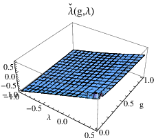
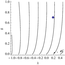
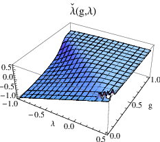
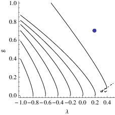
(B) Solving for the bare parameters. In Fig.3 we show the result of numerically solving (5.15) for the bare couplings as a function of the effective ones. One finds a well defined pair for all and . In the figure two values of or, equivalently of are employed. For the difference between bare and effective parameters is small, except close to the singular boundary at . The other example with is typical for moderately large values of where differs significantly from , but the map is still one-to-one. For extremely large values of the one-to-one correspondence breaks down (not shown). We shall not employ such values in the following.
(C) Bare fixed points. Next we apply the transformation to an “effective” RG trajectory. Since with the transformation has no explicit -dependence , the fixed point behavior is mapped onto an analogous fixed point behavior at the bare level: . The image of the GFP is always at , while the coordinates of the “bare” NGFP, and , depend on the value of . The NGFP is an inner point of the domain in which the map is defined and is differentiable. Its Jacobian matrix is non-singular there which entails that the critical exponents of the NGFP are identical for the “effective” and the “bare” flow. The same is not true for the GFP since it is located on the boundary of the corresponding space of couplings (see below).
(D) Phase portrait of the bare flow. In Fig.4 we present the result of applying the map to a set of representative “effective” RG trajectories on the half plane . Fig 4(a) shows the “effective” flow, while the plots (b),(c) and (d) correspond to the “bare” flow for three different values of Q. Since the map does not change the critical exponents of the NGFP, the bare trajectories, too, have the typical spiral form. However, contrary to the effective one, the bare cosmological constant at the NGFP can also be negative or zero for suitable choices of Q. Here we emphasize again that all choices are physically equivalent. Varying Q simply amounts to shifting contributions back and forth between the action and the measure.
(E) Vicinity of the GFP. Near the GFP we may expand the relation between bare and effective couplings. From (5.17) we obtain, in leading order, , along with
| (5.21) |
Inverting yields the bare quantities and
| (5.22) |
These expansions are the first few terms of a power-log series. They make it explicit that because of the logarithms of Newton’s constant the relationship between and is not analytic; it could not be found in a perturbation theory-like power series expansion about the GFP.
The -trajectories linearized about the GFP are given by [43, 39]
| (5.23) | ||||
| (5.24) |
where and are constants.77 7 The constants and are the coordinates at the “turning point” at which, by definition, . The parameter is the scale at which the trajectory passes this point [43, 39]. Inserting (5.23), (5.24), with replaced by into the above equations we obtain the “bare” trajectories near the GFP:
| (5.25) |
Here we abbreviated . Note that contains terms proportional to and , that is, the RG running of the bare cosmological and Newton constant near the GFP is not a pure power law but has logarithmic corrections. The analogous running at the effective level, eqs.(5.23), is of power law-type, however. This difference in behavior could not occur if the relation between bare and effective parameters was given by a smooth map. This condition fails to be satisfied on the line on which the GFP is situated.
To summarize: Both the “effective” and the “bare” NGFP are inner points of the corresponding coupling constant space. The flow in the vicinity of one is the diffeomorphic image of the flow near the other. The RG running of the respective scaling fields is and , respectively, with the same critical exponents . The “bare” GFP is located on the boundary of the domain on which the map from the effective to bare coupling is defined. In its vicinity (on the half plane with ) the “bare” running is characterized by logarithmically corrected power laws. The “effective” GFP, on the other hand, shows pure power law scaling.
| (a) | ||
 |
 | |
| (b) | ||
 |
 | |
| (c) | ||
 |
 | |
| (d) | ||
 |
 |
| (a) | (b) |
 |
 |
| (c) | (d) |
 |
 |
6 Summary, discussion, and outlook
(A) The reconstruction problem. In this paper we analyzed the problem of how, being given a running effective action, the underlying quantum system it stems from can be reconstructed. Working in a path integral context, we showed explicitly that, after specifying a UV regularization scheme and a measure, every solution of the flow equation for the effective average action (without an UV cutoff) gives rise to a regularized path integral, and to a (UV cutoff dependent) bare action in particular.
(B) Completing the Asymptotic Safety program. While the discussion is completely general, this work was motivated by the Asymptotic Safety program in Quantum Einstein Gravity. As to yet the investigations based upon the EAA focused on computing RG trajectories of the -free FRGE and establishing the existence of a non-Gaussian fixed point. The present work aims at completing the Asymptotic Safety program in the sense of (re)constructing the, yet unknown, quantum system which we implicitly quantize by picking a solution of the flow equation. In fact, in our approach the primary definition of “QEG” is in terms of an RG trajectory of the EAA that emanates from the fixed point. The advantage of this strategy, defining the theory in terms of an effective rather than bare action, is that it automatically guarantees an “asymptotically safe” high energy behavior. The disadvantage is that in order to complete the Asymptotic Safety program, that is, to find the underlying microscopic theory, extra work is needed.
(C) Towards a Hamiltonian description. Once we know the microscopic, i.e. bare action we can attempt a kind of “Legendre transformation” to find appropriate phase space variables, a microscopic Hamiltonian, and thus a canonical description of the bare theory. Only at this level we can identify the degrees of freedom that got quantized, as well as their fundamental interactions. Since the Hamiltonian is unlikely to turn out quadratic in the momenta, the “Legendre tansformation” involved is to be understood as a generalized, i.e. quantum mechanical one. In the simplest case it consists in reformulating a given configuration space path integral as a phase space integral . With other words, we must undo the integrating out of the momenta.
However, given the complexity of which most probably contains higher derivatives and non-local terms a generalized, Ostrogradski-type phase space formalism will emerge presumably.
Being interested in a canonical description of the “bare” NGFP action one might wonder if there exists an alternative formalism which deals directly with the RG flow of Hamiltonians rather than Lagrangians. It seems that there hardly can be a practicable approach of this kind which is similar in spirit to the EAA. The reason is as follows.
If we apply a coarse graining step to an action which contains only, say, first derivatives of the field, the result will contain higher derivatives in general. This poses no special problem in a Lagrangian setting, but for the Hamiltonian formalism it implies that new momentum variables must be introduced. As a result, the coarse grained Hamiltonian “lives” on a different phase space (in the sense of Ostrogradski’s method) than the original one. Therefore, at least in a straightforward interpretation, there is no Hamiltonian analog of the flow on the space of actions. For this reason there is probably no simple way of getting around the “reconstruction problem”.
However, the above discussion does not contradict other approaches where the renormalization procedure could be applied in a Hamiltonian description [56] since there the coarse graining is performed in space (rather than spacetime) only.
(D) Degrees of freedom vs. carrier fields. One should emphasize that it is by no means clear from the outset what kind of fundamental degrees of freedom will be found in this Hamiltonian analysis. In our approach the only nontrivial input is the theory space, the space of functionals on which the renormalization group operates. Having fixed this space a FRGE can be written down, the resulting flow can be computed, its fixed point(s) can be identified, and the associated asymptotically safe field theories can be defined without any additional input.88 8 Apart from the physically irrelevant details of the coarse graining scheme. As a consequence, the only statement about the degrees of freedom in these theories which we can make on general grounds is that they can be “carried” by precisely those fields on which depends. (In the case at hand, theory space contains all functionals which are invariant under diffeomorphisms.) Clearly, just knowing the carrier field but not the action, here , tells us comparatively little about the degrees of freedom99 9 Recall, for instance, how the structure of propagating modes changes when higher derivative or nonlocal terms are added to some conventional action.. The action , however, is a prediction of the theory, not an input. From this point of view it is quite nontrivial that QEG was found to have RG trajectories which indeed describe classical General Relativity on macroscopic scales.
(E) This work. In the present paper we took a few first steps towards solving the reconstruction problem. In particular we demonstrated that the information contained in the EAA without a UV cutoff is sufficient to define a regularized path integral representation of the underlying theory with a well defined limit .
The construction requires a certain amount of EAA technology which we provided in Section 2. In particular we explained why, using a nonsingular coarse graining operator , the EAA does not precisely correspond to the familiar picture of a momentum shell integration, a continuum analog of the Kadanoff-Wilson block spin transformation. For understanding how a solution of the -free FRGE, the corresponding solution of the FRGE with UV cutoff, and the bare action are interrelated it is important to appreciate this difference. In Section 2 we explained the relationship between and , and in Section 3 we showed how a given trajectory gives rise to a trajectory of bare actions. In Section 4 we illustrated the method in a technically simple context which is physically relevant in its own right, namely the running cosmological constant induced by a scalar matter field. We contrasted the running effective and bare cosmological constant and saw, for instance, that the former is always positive at high momentum scales, while the latter can be positive, negative, or even zero depending on the normalization of the measure. This is consistent with the interpretation of the effective one as the physical cosmological constant at a given scale, while its bare counterpart is completely unphysical and may not be used for purposes of RG improvement.
Finally, in Section 5, we investigated QEG in the Einstein-Hilbert truncation. We constructed the map relating the effective to the bare Newton and cosmological constant, and we analyzed the properties on the “bare” RG flow. We saw in particular that the “effective” NGFP maps onto a corresponding “bare” one; in its vicinity the scaling fields show a power law running with the same critical exponents as at the effective level. The situation is different for the GFP which is a boundary point of parameter space. The pure power laws of the “effective” flow receive logarithmic corrections on the “bare” side.
(F) Outlook: conformally reduced gravity. Before closing let us mention some extensions of the work described here. Clearly it would be interesting to construct the bare QEG action in a more general truncation. A first investigation in this direction [55] has been performed in the context of conformally reduced gravity [24, 25] in which only the conformal factor of the metric is quantized. The simplicity of the model allows for the use of comparatively general truncations. Using the local potential approximation in which the for the conformal factor is taken to be of the type with a running potential it has been shown [25] that there exists a NGFP on the infinite dimensional space of the ’s; the fixed point potential was found to be a pure -monomial (for the topology): .
Using the method of the present paper one can now determine the corresponding bare potential function ; one finds [55]
| (6.1) |
Remarkably, while this potential is of the familiar Coleman-Weinberg form, it is here part of the bare action; it corresponds to a simple monomial in the effective one . Thus, as compared to a standard scalar matter field theory, the situation is exactly inverted.
It is not difficult to understand how this comes about: The difference is given by a supertrace which is nothing but a differentiated one-loop determinant. As a consequence, and differ precisely by terms typical of a one loop effective action. For a scalar they include the potential term , but also nonlocal terms (not considered here) such as , say. Hence a term in unavoidably amounts to a Coleman-Weinberg term in , at least within the truncation considered.
(G) Outlook: Yang-Mills theory and nonlinear sigma models. Leaving aside gravity, in future work it will be interesting to analyze higher dimensional Yang-Mills theory along the same lines. In fact, in ref.[30] the effective average action of -dimensional Yang-Mills theory was considered in a simple -truncation. According to this truncation1010 10 For a generalization see also [57]., has a NGFP in the UV if . Inspired by the structure of the one-loop effective action in Yang-Mills theory one would expect that the “bare” counterpart of the -fixed point should contain terms like , and also nonlocal ones such as . For the following reason it is of some practical importance to find out whether this is actually the case in a sufficiently general, reliable truncation. It seems comparatively easy to perform Monte-Carlo simulations in , say, so that one could possibly get an independent confirmation of the results obtained from the average action. However, the problem is that a priori we do not really know which bare theory should be simulated in order to arrive at the lattice version of the average action results. The present analysis of this paper suggests that if Yang-Mills theory is asymptotically safe in , the effective fixed point action might be simple, but could contain “exotic” nonlinear and nonlocal terms. If so, it is conceivable that is sufficiently different from to belong to a new universality class. In this case a Monte-Carlo simulation based upon the conventional Wilson gauge field action might not find a NGFP, while it should show up when a discretized version of is used.
Completely analogous remarks apply to the nonlinear sigma model in which, according to the lowest order truncation of the EAA, is asymptotically safe too [58].
Acknowledgments. E.M. would like to thank the German Academic Exchange Service (DAAD) for support.
Appendix A Appendix
In this appendix we evaluate the functional trace appearing in eq.(5.10),
| (A.1) |
We perform the derivative expansion up to the second order.
Since the truncated functional has the same structure as the ansatz for , we can easily obtain the Hessian from by replacing and . The Hessian has been worked out in [6] in order to derive the FRGE so that we can take advantage of the results obtained there. As in [6], we partly diagonalize the matrix by pulling the trace out of the field , defining with and , and assuming the background metric to correspond to a sphere which, as in [6], means no loss of generality. As a result, the supertrace (.1) boils down to three separate traces over symmetric tensor fields, scalars, and vector fields, respectively. The operators and in the respective sectors can be read off from the formulae in Section 4 of ref.[6]. In this way we obtain
| (A.2) |
Here, denotes the regularized trace in the tensor, scalar, and vector sector, respectively, and the constants are defined as in [6]:
| (A.3) |
The first, second, and third trace in (.2) stems from the , , and the ghost fluctuations, respectively. As the background metric was identified with a sphere of radius , the curvature scalar in (.2) is given by . Our task is to expand the traces in powers of , retaining only the terms proportional to and . They allow us to unambiguously identify the prefactors and of and , respectively.
At this point we must pick a concrete function . We use the “optimized” cutoff defined in (2.23) since holds true exactly then. Under the traces of (.2) the eigenvalues of are restricted to be smaller than . Therefore (2.23) implies that, under the traces, . This leads to a considerable simplification:
| (A.4) | |||||
The derivative expansion of the traces involving the step function can be found with standard heat kernel techniques. Up to second derivatives of the metric it reads1111 11 This formula is most easily obtained by making use of eq.(4.27) in ref.[6] for the special case .
| (A.5) |
Here the algebraic trace counts the number of independent field components in the , and sectors; it equals , , and , respectively.
Now it is a matter of straightforward algebra to insert (.5) and (.3) into (.4), and to expand in powers of , noting that and . The final result for the supertrace is then indeed found to have the same structure as the RHS of (5.10) so that we can read off the coefficients and :
| (A.6a) | ||||
| (A.6b) | ||||
| (A.6c) | ||||
| (A.6d) | ||||
Here . For the above results reduce to those in the eqs.(5.14) of the main text.
References
- [1]
For a general introduction see C. Kiefer, Quantum Gravity, Second Edition,
Oxford Science Publications, Oxford (2007). - [2]
A. Ashtekar, Lectures on non-perturbative canonical gravity,
World Scientific, Singapore (1991);
A. Ashtekar and J. Lewandowski, Class. Quant. Grav. 21 (2004) R53. - [3] C. Rovelli, Quantum Gravity, Cambridge University Press, Cambridge (2004).
- [4]
Th. Thiemann, Modern Canonical Quantum General Relativity,
Cambridge University Press, Cambridge (2007). - [5]
S. Weinberg
in General Relativity, an Einstein Centenary Survey,
S.W. Hawking and W. Israel (Eds.), Cambridge University Press (1979);
S. Weinberg, hep-th/9702027. - [6] M. Reuter, Phys. Rev. D 57 (1998) 971 and hep-th/9605030.
- [7] D. Dou and R. Percacci, Class. Quant. Grav. 15 (1998) 3449.
- [8] O. Lauscher and M. Reuter, Phys. Rev. D 65 (2002) 025013 and hep-th/0108040.
- [9] M. Reuter and F. Saueressig, Phys. Rev. D 65 (2002) 065016 and hep-th/0110054.
- [10] O. Lauscher and M. Reuter, Phys. Rev. D 66 (2002) 025026 and hep-th/0205062.
- [11] O. Lauscher and M. Reuter, Class. Quant. Grav.19 (2002) 483 and hep-th/0110021.
- [12] O. Lauscher and M. Reuter, Int.J. Mod. Phys.A 17 (2002) 993 and hep-th/0112089.
- [13] W. Souma, Prog. Theor. Phys. 102 (1999) 181.
- [14] M. Reuter and F. Saueressig, Phys. Rev. D 66 (2002) 125001 and hep-th/0206145; Fortschr. Phys. 52 (2004) 650 and hep-th/0311056.
- [15] A. Bonanno and M. Reuter, JHEP 02 (2005) 035 and hep-th/0410191.
- [16]
For reviews see:
M. Reuter and F. Saueressig, arXiv:0708.1317 [hep-th],
O. Lauscher and M. Reuter in Quantum Gravity, B. Fauser,
J. Tolksdorf and E. Zeidler (Eds.), Birkhäuser, Basel(2007) and hep-th/0511260,
O. Lauscher and M. Reuter in Approaches to Fundamental Physics,
I.-O. Stamatescu and E. Seiler (Eds.), Springer, Berlin (2007). - [17]
R. Percacci and D. Perini,
Phys. Rev. D 67 (2003) 081503;
Phys. Rev. D 68 (2003) 044018; Class. Quant. Grav.21 (2004) 5035. - [18]
A. Codello and R. Percacci,
Phys. Rev. Lett.97 (2006) 221301;
A. Codello, R. Percacci and C. Rahmede, Int.J. Mod. Phys.A23 (2008); preprint arXiv:0805.2909 [hep-th]. - [19]
D. Litim,
Phys. Rev. Lett.92 (2004) 201301;
AIP Conf.Proc.841 (2006) 322;
P. Fischer and D. Litim, Phys. Lett. B 638 (2006) 497;
AIP Conf.Proc.861 (2006) 336. - [20] P. Machado and F. Saueressig, Phys. Rev. D 77 (2008) 124045.
- [21] O. Lauscher and M. Reuter, JHEP 10 (2005) 050 and hep-th/0508202.
- [22] M. Reuter and J.-M. Schwindt, JHEP 01 (2006) 070 and hep-th/0511021.
- [23] M. Reuter and J.-M. Schwindt, JHEP 01 (2007) 049 and hep-th/0611294.
- [24] M. Reuter and H. Weyer, preprint arXiv:0801.3287 [hep-th].
- [25] M. Reuter and H. Weyer, preprint arXiv:0804.1475 [hep-th].
- [26] J.-E. Daum and M. Reuter, preprint arXiv:0806.3907 [hep-th].
- [27]
P. Forgács and M. Niedermaier,
hep-th/0207028;
M. Niedermaier, JHEP 12 (2002) 066; Nucl. Phys. B 673 (2003) 131;
Class. Quant. Grav.24 (2007) R171. - [28]
For detailed reviews of asymptotic safety in gravity see:
M. Niedermaier and M. Reuter, Living Reviews in Relativity 9 (2006) 5;
R. Percacci, arXiv:0709.3851 [hep-th]. - [29] C. Wetterich, Phys. Lett. B 301 (1993) 90.
- [30] M. Reuter, C. Wetterich, Nucl. Phys. B 417 (1994) 181.
- [31]
M. Reuter and C. Wetterich,
Nucl. Phys. B 427 (1994) 291,
Nucl. Phys. B 391 (1993) 147, Nucl. Phys. B 408 (1993) 91; M. Reuter, Phys. Rev. D 53 (1996) 4430, Mod.Phys. Lett. A 12 (1997) 2777. - [32] M. Reuter and C. Wetterich, Nucl. Phys. B 506 (1997) 483.
- [33]
J. Berges, N. Tetradis and C. Wetterich,
Phys.Rep.363 (2002) 223;
C. Wetterich, Int.J. Mod. Phys. A 16 (2001) 1951. - [34]
For reviews of the effective average action in Yang–Mills theory see:
M. Reuter, hep-th/9602012; J. Pawlowski, hep-th/0512261;
H. Gies, hep-ph/0611146. - [35]
A. Bonanno and M. Reuter,
Phys. Rev. D 62 (2000) 043008 and hep-th/0002196;
Phys. Rev. D 73 (2006) 083005 and hep-th/0602159;
Phys. Rev. D 60 (1999) 084011 and gr-qc/9811026. - [36] M. Reuter and E. Tuiran, hep-th/0612037.
- [37]
A. Bonanno and M. Reuter,
Phys. Rev. D 65 (2002) 043508 and hep-th/0106133;
M. Reuter and F. Saueressig, JCAP 09 (2005) 012 and hep-th/0507167. - [38]
A. Bonanno and M. Reuter,
Phys. Lett. B 527 (2002) 9 and astro-ph/0106468;
Int. J. Mod. Phys. D 13 (2004) 107 and astro-ph/0210472;
E. Bentivegna, A. Bonanno and M. Reuter, JCAP 01 (2004) 001
and astro-ph/0303150. - [39] A. Bonanno and M. Reuter, JCAP 08 (2007) 024 and arXiv:0706.0174 [hep-th].
- [40]
A. Bonanno, G. Esposito and C. Rubano,
Gen. Rel. Grav. 35 (2003) 1899;
Class. Quant. Grav. 21 (2004) 5005;
A. Bonanno, G. Esposito, C. Rubano and P. Scudellaro,
Class. Quant. Grav. 23 (2006) 3103 and 24 (2007) 1443. - [41] M. Reuter and H. Weyer, Phys. Rev. D 69 (2004) 104022 and hep-th/0311196.
- [42] M. Reuter and H. Weyer, Phys. Rev. D 70 (2004) 124028 and hep-th/0410117.
- [43] M. Reuter and H. Weyer, JCAP 12 (2004) 001 and hep-th/0410119.
- [44] T. Appelquist and J. Carrazzone, Phys. Rev. D 11 (1975) 2856.
- [45]
F. Girelli, S. Liberati, R. Percacci and C. Rahmede,
Class. Quant. Grav.24 (2007) 3995. - [46] D. Litim and T. Plehn, Phys. Rev. Lett.100 (2008)131301.
- [47]
J. Moffat,
JCAP 05 (2005) 2003;
J.R. Brownstein and J. Moffat, Astrophys.J.636 (2006) 721;
Mon.Not.Roy.Astron.Soc.367 (2006) 527. - [48]
L.F. Abbott,
Nucl. Phys. B 185 (1981) 189;
B.S. DeWitt, Phys.Rev.162 (1967) 1195;
M.T. Grisaru, P.van Nieuwenhuizen and C.C. Wu, Phys. Rev. D 12 (1975) 3203;
D.M. Capper, J.J. Dulwich and M. Ramon Medrano, Nucl. Phys. B 254 (1985) 737;
S.L. Adler, Rev.Mod.Phys.54 (1982) 729. - [49]
R. Floreanini and R. Percacci,
Nucl. Phys. B 436 (1995) 141;
Phys. Rev. D 46 (1992) 1566. - [50]
D. Litim,
Phys. Lett.B 486 (2000) 92;
Phys. Rev. D 64 (2001) 105007;
Int.J. Mod. Phys.A 16 (2001) 2081. - [51]
H.W. Hamber, Phys. Rev. D 45 (1992) 507;
Phys. Rev. D 61 (2000) 124008; arXiv:0704.2895 [hep-th];
T. Regge and R.M. Williams, J.Math.Phys.41 (2000) 3964 and gr-qc/0012035. - [52] J. Ambjørn, J. Jurkiewicz and R. Loll, Phys. Rev. Lett.93 (2004) 131301.
- [53] J. Ambjørn, J. Jurkiewicz and R. Loll, Phys. Lett.B 607 (2005) 205.
- [54]
J. Ambjørn, J. Jurkiewicz and R. Loll,
Phys. Rev. Lett.95 (2005) 171301;
Phys. Rev. D 72 (2005) 064014; Contemp.Phys.47 (2006) 103. - [55] E. Manrique and M. Reuter, work in progress.
- [56]
E. Manrique, R. Oeckl, A. Weber and J. A. Zapata,
Class. Quant. Grav. 23 (2006) 3393 and
hep-th/0511222;
A. Corichi, T. Vukasinac and J. A. Zapata, Class. Quant. Grav. 24 (2007) 1495 and gr-qc/0610072. - [57] H. Gies, Phys. Rev. D 68 (2003) 085015.
- [58] A. Codello and R. Percacci, arXiv:0810.0715 [hep-th].