Coleman-de Luccia Tunneling and the Gibbons-Hawking Temperature

Tunneling in the presence of gravity was first beautifully analyzed by Coleman and de Luccia (CDL) [1]. This problem emerges in the study of the early universe in relation to the inflationary epoch, and more recently, in relation to the cosmic landscape as suggested by superstring theory. However, there are properties of the CDL tunneling that remain to be better understood.

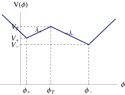
Consider a simplified theory of a single scalar field with potential $V(\phi)$ and a canonical kinetic term in the presence of gravity. The potential $V(\phi)$ has a false vacuum $V_{+}$ at $\phi_{+}$ and a true vacuum $V_{-}$ at $\phi_{-}$, so the energy density difference between them is $\epsilon=V_{+}-V_{-}>0$. The potential barrier between these two local minima has height $V_{T}$, as shown in Figure 1.

In the semiclassical approximation, the tunneling rate per unit volume is given by

where $S_{E}(\phi)$ is the Euclidean action for the bounce solution and $S_{E}(\phi_{+})$ is the Euclidean action evaluated at the false vacuum at $\phi_{+}$. In the thin-wall approximation ($\epsilon\rightarrow 0$), when the vacuum energy density is negligible compared to the Planck scale, $B$ recovers the result in the absence of gravity [2], as expected. On the other hand, as we increase $V_{+}\gtrsim V_{-}$, while still in the thin-wall approximation [3], $B$ takes a different form,

where $\tau$ is the domain wall tension and the Hubble constant is given by $H^{2}=8\pi G_{N}V_{+}/3=V_{+}/3M_{p}^{2}$. Note that the first form (when $V_{+}$ is small) is independent of $V_{+}$ while the second form is independent of $\epsilon=V_{+}-V_{-}$. We see that, for fixed $\tau$, $B$ decreases rapidly as $H$ increases. It seems that we can easily have a situation where $B\ll 1$, in which case, the tunneling is not exponentially suppressed at all (and the evaluation of the prefactor $A$ in (1) as well as sub-dominant contributions to $\Gamma$ becomes important).

A similar phenomenon seems to be happening in the Hawking-Moss (HM) tunneling [4],

where $\Delta V_{+}=V_{T}-V_{+}$. Note that if we move $V(\phi)$ up without changing its shape, that is, keeping $\epsilon$, $\tau$ and $\Delta V_{+}$ fixed, $B$ decreases like $H^{-3}$ or $H^{-4}$, depending on which formula (i.e., thin wall or HM) is applicable. In this paper, we like to see if and under what conditions this phenomenon is real. More precisely, we examine the CDL tunneling more generally to see when the thin-wall approximation or the HM formula (4) is valid.

CDL tunneling concerns quantum fluctuations in the false vacuum of a nucleation bubble which subsequently grows classically. The following picture emerges. Depending on the properties of $V(\phi)$, there are four regions in the parameter space, yielding four different situations how the nucleation bubble is created :

(I) The center of the nucleation bubble is in the true vacuum $V_{-}$ while the outside of the bubble reaches the false vacuum $V_{+}$. The thin-wall approximation is a special limit ($\epsilon\rightarrow 0$) in this case.

(II) The outside of the bubble reaches the false vacuum $V_{+}$ but the inside of the nucleation bubble never reaches the true vacuum $V_{-}$ in the Euclidean solution. After the creation of the bubble, its inside falls towards the true vacuum $V_{-}$ as the bubble grows.

(III) The inside of the bubble reaches $V_{-}$, but the outside of the bubble does not reach the false vacuum in the Euclidean action, due to the presence of the de Sitter horizon.

(IV) Not only does the inside of the bubble not reach $V_{-}$, the outside of the bubble does not reach the false vacuum in the Euclidean action, due to the presence of the de Sitter horizon. HM tunneling is a special limit in this case.

In the absence of gravity, regions faraway from the bubble are by definition in the false vacuum, so we have only case (I) and (II). In the presence of gravity, the de Sitter horizon cut off the scalar field $\phi$ as it tries to reach the false vacuum at large distance from the nucleation bubble [5]. That is why case (III) and (IV) are possible. This phenomenon of cases (III) and (IV) may be interpreted as a Gibbons-Hawking (GH) temperature $T_{H}=H/2\pi$ effect. This point was recently made by Brown and Weinberg [6], who show that tunneling in the presence of gravity may be interpreted as a combination of thermal (Gibbons-Hawking temperature) fluctuation plus quantum tunneling. We agree with this picture. That is, $\phi$ thermally fluctuates from the false vacuum at $\phi_{+}$ part way up the potential (to $\phi_{f+}$) before quantum tunneling to the other side of the barrier. In the Hawking-Moss limit, it fluctuates all the way to the top of the barrier at $V_{T}$. Here, our explicit calculations (in particular, the determination of $\phi_{f+}$) allow us to estimate in some detail, for a given potential, the individual contribution of the thermal fluctuation versus that of the quantum tunneling in the tunneling rate. We also evaluate the back-reaction effect on the background geometry and show that it can be very important.

There are a few other properties that are worth mentioning here.

$\bullet$ The thin-wall approximation is valid only when the tunneling belongs to case (I). In addition to the case (I) conditions (to be specified), we see that $M_{P}^{4}\gg V_{T}\gg\Delta V_{+}\gg\epsilon$. As we increase $V_{T}$ with a generic fixed shape of $V(\phi)$ (with $\epsilon>0$), the tunneling goes over to case (IV) via case (II) and/or case (III).

$\bullet$ For large $V_{T}$ and $\epsilon>0$, case (IV) is generic, where HM tunneling is a special limit. Here we estimate the accuracy of the HM formula (4) and its correction. We see that the HM formula for $B$ is an over-estimate, by as much as a factor of three. That is, the actual decay is a combination of thermal tunneling and quantum tunneling, whose rate can be much faster.

$\bullet$ Another interesting point is that tunneling in the absence of gravity is always downwards, while gravitational effects allow tunneling upwards.

$\bullet$ With an overall picture, we see that the fast drop off of $B$ as $H$ increases is real. This is illustrated in Figure 2, where case (III) does not appear due to the particular choice of the potential used.

$\bullet$ Strictly speaking, for a “general” smooth potential with varying parameters, the above four cases may reduce to case (IV) only. However, within case (IV), it contains regions that resemble the various cases discussed above. The triangular potential has four different cases so it actually demonstrates the change from thin wall to HM case more dramatically (but does not change the physics qualitatively.)

$\bullet$ As $B$ decreases, multi-nucleation bubbles will form and the phase transition involves bubble collisions. Once $B$ is small (say $B\lesssim 1$), Eq.(1) is no longer valid. The prefactor and sub-leading terms will become important. All we can say is that tunneling is no longer exponentially suppressed. The rate of transition depends on the details. We do expect that O(4) nucleation bubbles no longer dominate. That is, bubbles of other shapes as well as bubble collisions become important. The transition can be complicated and is at a fast time scale. Something analogous to spinodal decomposition may happen.

In terms of pure thermal (Gibbons-Hawking (GH) temperature) tunneling the suppression of the tunneling is interpreted as due to the Boltzmann factor, where the bubble is a 3-sphere and the inverse temperature is treated as an imaginary time with period $1/T_{H}$. In case (I) and (II), we see that the quantum tunneling is dominant (i.e., has a smaller value) due to the $O(4)$ symmetry that is lacking in the finite temperature effect. So strictly speaking, the enhancement of the tunneling rate due to a large vacuum energy density is a pure gravitational effect. In de Sitter-like vacua, we may interpret this as a GH temperature effect in the presence of an enhanced (here $O(4)$) symmetry. In case (III) and (IV), the GH temperature starts to play a more prominent role.

The same GH temperature will also contribute to the finite temperature effect on the potential $V(\phi)\rightarrow V(\phi,T_{H})$ [7, 8]. This contribution is perturbative in the couplings while its effect in tunneling is non-perturbative. In the finite temperature formalism, this leads to a term of the form $T_{H}^{2}\phi^{2}$ into the finite temperature potential. In the gravity perspective, this is simply a coupling of the form $R\phi^{2}$, where $R$ is the Ricci scalar. One an also interpret this as a finite volume effect, due to Gauss’s law, $H^{2}\phi^{2}$, where $H^{-1}$ is the horizon size. The overall picture is self-consistent and clear.

We shall comment on the impact of the GH temperature on the cosmic landscape, both on the shape of the effective potential of the landscape and on the tunneling rate. Because of fast tunneling when the wavefunction of the universe is high up in the landscape, it is likely that the universe is quite mobile there.

For a general potential $V(\phi)$, the coupled equations of $\phi(\xi)$ and the cosmic scale factor $r(\xi)$ are too complicated to solve even in the absence of the gravity except in the thin-wall approximation. However, for some special potentials, say, the triangular potential $V(\phi)$ (Figure 3), the bounce $B$ can be obtained analytically [9]. So it is natural to consider the tunneling rates for such a potential in the presence of gravity. Unlike Ref.[9], we cannot get an exact analytic formula for $B$ in the presence of gravity, but the resulting analytic study gives a very good approximation and does simplify enough for us to see the overall picture. Here the absolute height of the potential, which corresponds to the vacuum energy density, is important for tunneling with gravity. To be specific, we shall adopt this triangular potential in this paper.

The rest of the paper is organized as follows. In Sec. 2, we briefly review the overall framework of tunneling in de Sitter space. This framework is the CDL tunneling formalism. In Sec. 3, we go back to tunneling in the absence of gravity. In particular, we review the special case of tunneling in a triangular potential studied by Duncan and Jensen [9]. Here we emphasize the formulation that is suitable in the extension of their analysis to include gravity. Sec. 4 presents the setup for tunneling in de Sitter space, again using the triangular potential. As $\phi$ varies, the tunneling is not happening in pure de Sitter space and the back-reacrtion is estimated. Sec. 5 presents the main result of this paper. The above four cases and their conditions are discussed. The meaning and implications of the results are discussed in Sec. 6. We then discuss thermal tunneling in Sec. 7. Here we are referring to the treatment of the de Sitter horizon effect as a Gibbons-Hawking temperature effect. In Sec. 8, we point out that the Gibbons-Hawking temperature should also modify the potential via finite temperature effect on potentials. We then consider the implication of the Gibbons-Hawking temperature on the cosmic landscape. Sec. 9 contains the summary and some remarks.

Let us consider the theory of a single scalar field $\phi$ with a potential $V(\phi)$ in the presence of gravity, given by

where $\kappa=8\pi G=1/M_{p}^{2}$.

The potential $V(\phi)$ has a false vacuum $V_{+}$ at $\phi_{+}$ and a true vacuum $V_{-}$ at $\phi_{-}$. There is a potential barrier between these two local minima, as shown in Figure 1. Let the height of the barrier at $\phi_{T}$ be $V_{T}$. We have chosen $\phi_{-}>\phi_{T}>\phi_{+}$. Let the energy density difference between the false and the true vacua be $\epsilon=V_{+}-V_{-}>0$.

In the presence of gravity, the CDL tunneling rate per unit volume is given by Eq. (1,2), in term of the coefficient $B=S_{E}(\phi)-S_{E}(\phi_{+})$, where $S_{E}(\phi)$ is the Euclidean action for the bounce solution and $S_{E}(\phi_{+})$ is the Euclidean action evaluated at the false vacuum. Since a Euclidean solution with a $O(4)$ symmetry has an etremum action, $B$ is in general dominated by the “bounce” solution with $O(4)$ symmetry. This solution has the Euclidean metric,

where $d\Omega^{2}_{s}$ is the metric of a unit 3-sphere. The Euclidean equation for the “bounce” solution is determined by the minimum value of the Euclidean action,

where the prime is derivative with respect to $\xi$. Here the Einstein equation yields one non-trivial equation, since the equation of motion for $r(\xi)$ follows from Eqs. (7,8). We can choose $r(0)=0$. Using Eq.(8) to simplify the Euclidean action, one obtains

The CDL instanton is a unique solution with the topology of a four sphere $S^{4}$ in Euclidean space [10]. The geometry after bubble nucleation is described by the analytic continuation of the CDL instanton to Lorentzian signature. The radial coordinate $\xi$ is continued to $\xi=it$ and the metric in Lorentzian frame is

here the metric is multiplied by an overall minus sign and $d\Omega_{H^{3}}$ is the element of length for a unit hyperboloid with timelike normal. The metric within the spherical bubble describes a spatially open Friedmann-Robertson-Walker Universe.

As we shall see, a qualitative picture emerges: depending on the properties of the potential, there are four different cases how the nucleation bubble is created :

(I) The center of the nucleation bubble reaches the true vacuum $V_{-}$ while the outside of the bubble reaches the false vacuum $V_{+}$. The thin-wall approximation is a special limit ($\epsilon\rightarrow 0$) in this case.

(II) The outside of the bubble reaches the false vacuum $V_{+}$ but the inside of the nucleation bubble never reaches the true vacuum $V_{-}$ in the Euclidean solution. After the creation of the bubble, its inside will fall towards the true vacuum $V_{-}$ as the bubble grows.

(III) The inside of the bubble reaches $V_{-}$, but the outside of the bubble does not reach the false vacuum $V_{+}$ in the Euclidean action, due to the presence of the de Sitter horizon. This case and the next case never happen in the absence of gravity, since we start with the false vacuum everywhere. Far from the bubble, $\phi$ approaches the false vacuum by definition. However, when the vacuum energy is not negligible, there is a de Sitter horizon so it is possible that $\phi$ hits the horizon before it reaches the false vacuum.

(IV) Not only does the inside of the bubble not reach $V_{-}$, the outside of the bubble does not reach the false vacuum in the Euclidean action. The HM tunneling is the limit in this case. Here we are able to estimate the accuracy of the Hawking-Moss formula and its correction, which can be substantial.

For a general potential $V(\phi)$, the coupled equations (7, 8) are complicated to solve. In the absence of the gravity, for some simple potentials, say, the triangular potential $V(\phi)$ (Figure 3), the bounce $B$ can be obtained analytically [9]. Then it is natural to consider the tunneling rates for such potentials in the presence of the gravity. Unlike Ref.[9], we cannot get an analytical formula for $B$ in the presence of gravity, but the analysis does simplify enough for us to see the overall picture. Here the absolute height of the potential, which corresponds to the vacuum energy density, is important for tunneling with gravity. To be specific, we shall adopt this triangular potential in this paper.

The triangular potential may be parametrized in the following way. Let the height of the barrier of $V(\phi)$ at $\phi_{T}$ be $V_{T}$, which also provides a measure of the overall vacuum energy density. Let $\Delta V_{\pm}=(V_{T}-V_{\pm})$. Both $\Delta\phi_{+}=\phi_{T}-\phi_{+}$ and $\Delta\phi_{-}=\phi_{-}-\phi_{T}$ are defined to be positive so the slopes (gradients) $\pm\lambda_{\pm}$ of $V(\phi)$ are given by

Note that, in general, $\lambda_{+}\neq\lambda_{-}$. Since the $\epsilon={\Delta V_{-}}-{\Delta V_{+}}>0$, we have

$\Delta\phi_{+}$, $\Delta\phi_{-}$ and $\lambda$. Here, to simplify the solution, we set $\lambda_{L}=\lambda_{R}=\lambda$.

When gravity is negligible, Eq. (8) reduces to $r^{\prime}=1$. This happens if we set $\kappa=0$. Alternatively, this is a very good approximation when the overall height of the potential is much smaller than the Planck scale.

With $r(\xi=0)=0$, we have $r=\xi$, so tunneling reduces to the simple case without gravity. The solution must satisfy the boundary condition,

which is necessary for $\phi$ to make sense at the center of the nucleation bubble. At large radius, we expect

As we shall see, this condition may be modified when gravity is important.

Let us first review the solution to the triangular potential without gravity, the case worked out by Duncan and Jenson [9]. For $\phi_{+}\leq\phi\leq\phi_{-}$, Eq.(7) becomes

The general solution is

where the constant $a$ and $b$ are determined by the boundary conditions and by matching the field values and their derivatives at the top of the barrier, which occurs at some radius $\xi_{T}$ to be determined.

It is easy to see that $\phi$ will reach its false vacuum value at finite radius $\xi_{+}$ (to be determined) and then stay there. The above boundary condition (14) is replaced by

while there are two possibilities to satisfy the condition (13). The first case, namely case (I), is when $\phi$ stays close to $\phi_{-}$ until at radius $\xi_{-}$ when $\phi$ starts to decrease under Eq.(15). The boundary conditions in this case are

The other possibility, namely case (II), happens when, at the time of creation, the inside of the bubble never reaches the true vacuum. In this case, the boundary conditions are

where the initial value $\phi_{0}$ is to be determined. This case only happens if $\phi_{0}$ is to the right side of the barrier (i.e., near $\phi_{-}$) and $\phi_{0}\leq\phi_{-}$. Also, we expect $V_{+}\geq V(\phi_{0})\geq V_{-}$.

Let us now turn on gravity [1], so the triangular potential has five parameters, namely ($\Delta V_{\pm}$, $\Delta\lambda_{\pm}$, $V_{T}$). As noted above, at times, it may be convenient to choose an alternative but equivalent set of parameters.

To emphasize the effect of gravity, let us consider the situation where

where $V_{T}/M_{P}^{4}\ll 1$ so gravitational effects can be important for the tunneling while the semi-classical approximation is still valid.

The equation (7) now reads,

where $L=\phi^{\prime 2}/2-V+V_{T}$ is the (shifted) Euclidean energy. By (34), for large $V_{T}$, we use the approximation

where

is the Hubble constant of the de Sitter space with vacuum energy $V_{T}$. So we have

where $r(0)=r(\pi/H)=0$. That is, the range of $\xi$ is bounded, $0\leq\xi\leq\pi/H$.

It is easy to check that this approximation is self-consistent, i.e., $\big|L(\xi)\big|\ll V_{T}$. For a tunneling solution, $\phi(\xi)\in[\phi_{-},\phi_{+}]$, so

Using Eq.(7),

When $\xi\in[0,\pi/2H)$, $L^{\prime}\leq 0$ and if $\xi\in(\pi/2H,\pi/H]$, $L^{\prime}\geq 0$. Therefore $\max{L}=\max\{L(0),L(\pi/H)\}\leq\Delta V_{-}$. So $|L|\ll V_{T}$, and Eq.(38) is valid to the leading order in $\Delta V_{-}/V_{T}$, For later purposes, we note that

The equations (7, 8) are now decoupled, and

and can be solved with appropriate boundary conditions. This we shall do in the next section.

The bounce solution $\phi(\xi)$ will modify the geometric background used, i.e., $r(\xi)$ in (38). As we shall see, it is important to include this back-reaction. Inserting $\phi(\xi)$ back into Eq.(35), we get a first-order differential equation of the leading-order correction of $r$, namely $\delta r(\xi)$,

The formal solution for $\delta r$ is,

where the superficial singularity at $\eta=\pi/(2H)$ can be regularized as

Notice that by (40), $L^{\prime}(\pi/2H)=0$ and the integral is well defined. Now we can consider the Euclidean action for this solution, to the leading order of $\Delta V_{-}/V_{T}$,

We separate the result into three parts. The first part (46) is $-24\pi^{2}M_{p}^{4}/V_{T}$, the de-Sitter space Euclidean action. The second part (47) is suppressed by a small factor $\Delta V_{-}/V_{T}$ comparing with the first part, because by (45) the magnitude of $\delta r$ is of $H^{-1}\Delta V_{-}/V_{T}$, and the magnitude $V(\xi)-V_{T}$ is at most $\Delta V_{-}$. We will explicitly see that the two terms in the second part, which correspond to $\delta r$ and $\phi$ contribution are of the same order and therefore the computation of $\delta r(\xi)$ in Eq. (45) is important. The last part represents all the high order terms of $\Delta V_{-}/V_{T}$. Notice that by the perturbation $\delta r$, $\xi_{max}$ is no longer $\pi/H$. However, the action change induced by $(\xi_{max}-\frac{\pi}{H})$ is of the second order of the $\Delta V_{-}/V_{T}$ and hence is included in (48).

In conclusion, if we can get the analytic solution of (42) then the leading order of $r$ is immediately given by the integral in (45). It then follows that (46) and (47) give the leading order Euclidean action. Subtracting $S_{E}(\phi_{+})$ given by(41) from it, we get the factor $B$.

In general, Eq. (49) is still too difficult to solve in a way that the physics is transparent. However, for the triangle potential, we can solve (49) analytically. For the different choices of the five parameters $V_{T}$, $\Delta\phi_{+}$, $\Delta\phi_{-}$, $\lambda_{\pm}$, we find here are four different kinds of Euclidean solutions for $\phi$ (shown in Figure 4) :

• •

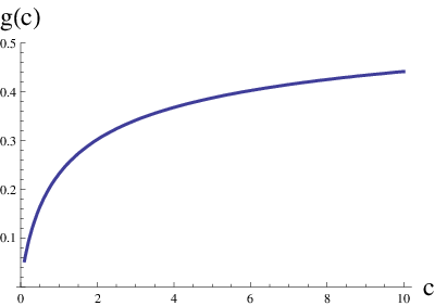
  Case (I) $\phi(\xi)$ reaches both $\phi_{+}$ and $\phi_{-}$. This happens when $\alpha\lambda/{H^{2}\Delta\phi_{+}}\geq 1$ and $(\lambda/{H^{2}})I\big(H^{2}\Delta\phi_{+}/{\lambda}\big)\geq\Delta\phi_{-}$ where $\alpha\sim 0.4$ and $I(x)$ is a monotonic function shown in Figure 6.

• •

  Case (II) $\phi(\xi)$ reaches $\phi_{+}$ but not $\phi_{-}$. That is, $\phi(\xi)$ reaches $\phi_{+}$ and $\phi_{t-}$, where $\phi_{T}\leq\phi_{t-}<\phi_{-}$. This happens when both $\alpha{\lambda}/{H^{2}\Delta\phi_{+}}\geq 1$ and $({\lambda}/{H^{2}})I\big({H^{2}\Delta\phi_{+}}/{\lambda}\big)<\Delta\phi_{-}$ are satisfied.

• •

  Case (III). $\phi(\xi)$ reaches $\phi_{-}$ but not $\phi_{+}$. That is, $\phi(\xi)$ reaches $\phi_{f+}$, where $\phi_{T}\geq\phi_{f+}>\phi_{+}$. This case can happen only when the gradient towards the true vacuum is steeper than that towards the false vacuum.

• •

  Case (IV). $\phi(\xi)$ reaches neither $\phi_{+}$ nor $\phi_{-}$. That is, $\phi(\xi)$ reaches only $\phi_{f+}$ and $\phi_{t-}$. This case happens when ${\alpha\lambda}/{H^{2}\Delta\phi_{+}}<1$ is satisfied.

In the absence of gravity, the triangle potential just has two kinds of bounce solutions [9], the cases (I) and (II). Here, including gravity, we have a new bounce solution, either case (III) or case (IV), because here there is a cut-off $\xi_{max}$ of the radius coordination $\xi$ due to the Hubble radius of de Sitter space. So in the finite range $0\leq\xi\leq\pi/H$, the bounce solution may reach neither $\phi_{+}$ nor $\phi_{-}$. We will see that case (IV) is like HM tunneling, the case (I) is like thin-wall CDL tunneling, and case (II) is an intermediate case between the two limits. By adjusting the five parameters of the potential, we get a transition from HM tunneling to thin-wall CDL tunneling.

For the triangular potential $V(\phi)$ shown in Figure 3, we have, for large $V_{T}$,

whose general solution is given by

where $f_{1}(H\xi)$ is the special solution and $f_{2}$ is the homogeneous solution.

Note that $f_{2}^{\prime}(H\xi)=H/\sin^{3}(H\xi)$. The constants $a_{1}$ and $b_{1}$ are to be determined by the boundary and matching conditions. We begin our discussion with case (IV) since it is new and its limiting case corresponds to HM tunneling.

References

- [1] S. R. Coleman and F. De Luccia, “Gravitational Effects On And Of Vacuum Decay,” Phys. Rev. D 21, 3305 (1980).
- [2] S. R. Coleman, “The Fate Of The False Vacuum. 1. Semiclassical Theory,” Phys. Rev. D 15, 2929 (1977) [Erratum-ibid. D 16, 1248 (1977)].
- [3] Q.-G. Huang and S.-H. H. Tye, “The cosmological constant problem and inflation in the string landscape,” ArXiv:0803.0663 [hep-th].
- [4] S. W. Hawking and I. G. Moss, “Supercooled Phase Transitions In The Very Early Universe,” Phys. Lett. B 110, 35 (1982).
- [5] L. G. Jensen and P. J. Steinhardt, “Bubble nucleation and the Coleman-Weinberg model.” Nucl. Phys. B 237, 176 (1984).
- [6] A. R. Brown and E. J. Weinberg, “Thermal derivation of the Coleman-De Luccia tunneling prescription,” Phys. Rev. D 76, 064003 (2007) [arXiv:0706.1573 [hep-th]].
- [7] B. Allen, “Phase Transitions in de Sitter Space,” Nucl. Phys. B 226, 228 (1983).
- [8] G. L. Kane, M. J. Perry, A. N. Zytkow, “Spontaneous Symmetry Breaking and Tunneling in de Sitter Space,” [arXiv:hep-th/0407217v2].
- [9] M.J. Duncan and L. G. Jensen, “Exact tunneling solutions in scalar field theory” Nuclear physics B 291, 109 (1992).
- [10] E. Mottola and A. Lapedes “Existence of finite-action solutions to the Coleman-De Luccia equations” Phys. Rev. D 29, 773 (1984).
- [11] V. Gen and M. Sasaki, “False vacuum decay with gravity in non-thin-wall limit,” Phys. Rev. D 61, 103508 (2000) [arXiv:gr-qc/9912096].
- [12] A. S. Goncharov and A. D. Linde, “Tunneling in an expanding universe: Euclidean and Hamiltonian approaches,” Sov. J. Part. Nucl. 17 369 (1987).
- [13] A. A. Starobinsky, “Stochastic DeSitter (Inflationary) Stage in the Early Universe,” in Field Theory, Quantum Gravity and Strings, edited by H.J. De Vega and N. Sanchez (Springer New York 1986).
- [14] A. S. Goncharov, A. D. Linde and V. F. Mukhanov, “The Global Structure of the Inflationary Universe,” Int. J. Mod. Phys. A 2, 561 (1987).
- [15] K. Lee and E. J. Weinberg, “Decay of the true vacuum in curved space-time,” Phys. Rev. D 36, 1088 (1987).
- [16] B. H. Lee and W. Lee, “The vacuum bubble and black hole pair creation,” ArXiv:0809.4907v2 [hep-th].
- [17] S. Parke, “Gravity and the decay of the false vacuum,” Phys. Lett. B 121, 313 (1983).
- [18] E. J. Weinberg, “Hawking-Moss bounces and vacuum decay rates,” Phys. Rev. Lett. 98, 251303 (2007). [arXiv:hep-th/0612146].
- [19] I. Affleck, “Quantum-Statistical Metastability,” Phys. Rev. Lett. 46, 388 (1981).
- [20] C. G. Callan and S. R. Coleman, “Fate of the false vacuum. II. First quantum corrections,” Phys. Rev. D 16, 1762 (1977).
- [21] A. D. Linde, Nucl. Phys. B 216, 421 (1983); [Erratum: B 223, 544 (1983)].
- [22] S. Kachru, R. Kallosh, A. D. Linde and S. P. Trivedi, “de Sitter vacua in string theory,” Phys. Rev. D 68, 046005 (2005) [arXiv:hep-th/0301240].
- [23] R. Easther and L. McAllister, “Random Matrices and the Spectrum of N-flation,” [arXiv:hep-th/0512102].
- [24] P. Svrcek and E.Witten, “Axions in String Theory,” JHEP 0606, 051 (2006), arxiv:0605206 [hep-th].
- [25]
S. Kachru, R. Kallosh, A. Linde, J. Maldacena, L. McAllister
and S. P. Trivedi,
“Towards inflation in string theory,”
JCAP 0310 (2003) 013, hep-th/0308055;
S. Shandera, B. Shlaer, H. Stoica and S.-H. H. Tye, “Inter-brane interactions in compact spaces and brane inflation,” JCAP 0402, 013 (2004), hep-th/0311207. - [26] S.-H. H. Tye, “A new view of the cosmic landscape,” ArXiv:hep-th/0611148.
- [27] S.-H. H. Tye, “A Renormalization Group Approach to the Cosmological Constant Problem,” ArXiv:0708.4374 [hep-th].