Temporal Support of Regular Expressions in Sequential Pattern Mining
Abstract
Classic algorithms for sequential pattern discovery, return all frequent sequences present in a database. Since, in general, only a few ones are interesting from a user’s point of view, languages based on regular expressions (RE) have been proposed to restrict frequent sequences to the ones that satisfy user-specified constraints. Although the support of a sequence is computed as the number of data-sequences satisfying a pattern with respect to the total number of data-sequences in the database, once regular expressions come into play, new approaches to the concept of support are needed. For example, users may be interested in computing the support of the RE as a whole, in addition to the one of a particular pattern. Also, when the items are frequently updated, the traditional way of counting support in sequential pattern mining may lead to incorrect (or, at least incomplete), conclusions. For example, if we are looking for the support of the sequence A.B, where A and B are two items such that A was created after B, all sequences in the database that were completed before A was created, can never produce a match. Therefore, accounting for them would underestimate the support of the sequence A.B. The problem gets more involved if we are interested in categorical sequential patterns. In light of the above, in this paper we propose to revise the classic notion of support in sequential pattern mining, introducing the concept of temporal support of regular expressions, intuitively defined as the number of sequences satisfying a target pattern, out of the total number of sequences that could have possibly matched such pattern, where the pattern is defined as a RE over complex items (i.e., not only item identifiers, but also attributes and functions).
1 Introduction
Traditional sequential patterns algorithms are founded on the assumption that items in databases are static, and that they existed throughout the whole lifespan of the world modeled by the database. There are many real-world situations where sequential pattern mining (SPM) is usually applied, and where these assumptions are not valid any more. In these situations, items are created or deleted dynamically. Further, if we are interested in categorical SPM, we need to deal with complex items, i.e., items described by attributes (or even functions over attributes). These attributes are also usually subject to change. Consider for example SPM in trajectory databases. For many applications, we may be interested in trajectory patterns involving restaurants, hotels, gas stations. The features that characterize these places may change over time, and even many of them could have not existed when some of the trajectories under analysis occurred. This may also occur in the context of the World Wide Web, where Web pages are frequently added or deleted. Ntoulas et al. [10] collected snapshots over 155 web sites, during one year, once a week. They concluded that new pages are created at the rate of 8% per week, and only 20% of the pages available at one instant will be accessible after one year. Thus, there ia a high frequency of creation and deletion of Web pages. Moreover, they found that the link structure of the Web is more dynamic that the page content.
We introduce the problem through a Web usage mining example. Data Mining techniques have been applied for discovering interaction patterns of WWW users. Typically, this mining is performed over the URLs visited during a session, recorded in a Web server log. In this way, the interests and behavioral patterns of Web users can be studied. Figure 1 depicts a portion of a (simplified) Web log. In classic SPM, the support of a sequence is defined as the fraction of sessions that support . Thus, all sessions are considered as having the same probability to support a given sequence. For example, the support of the sequence CBC, counted in the classical way, would be 66%, since CBC is present in two of the three sessions. Analogously, the support of the sequence CB would also be 66%. We may ask would have happened if not all these Web pages existed all the time. The question is: would it be realistic to count support in the usual way? More precisely, would it be reasonable to ignore the evolution of the items (URLs) across time? We discuss these issues in this paper.
When a Web page is visited during a session, it is often the case where a user clicks a nonexisting link or a link that has been removed. Figure 2 shows how URLs A, B, and C in Figure 1, have evolved, and the time intervals when each URL has been available. We can see that URL A was available during the interval [1, 8], URL B in intervals [4, 5] and [11, now], and URL C, during [3, 6] and [9, now]. (We use the term now to refer to the current time instant). We now analyze the support of the sequence CBC. During session s2, we can see that URL C did not exist at t=8, when the user clicked URL A. Thus, session s2 did not have the possibility of producing a sequence that finishes with the URL C. Sessions s1 and s3, instead, support the sequence CBC. Then, ignoring the evolution of these URLs, the support of sequence CBC would be 66%, but, if we do not count session s2, we would obtain a support of 100% for this sequence. Analogously, if we compute the support of the sequence of CB taking into account the availability of the items during each session, we can see that s1 and s3 support this sequence, but s2 does not. However, C was available during session s2, when the user clicked URLs A (t=3) and B (t=4) (actually, it existed in the interval [3, 6]). Thus, the user could have produced the sequence CB, although she decided to follow a different path. Session s2 must then be counted for computing the support of the sequence CB, which would be 66%.
The example above gives the intuition of the ideas that we discuss and formalize in this paper: the support of a sequence depends on the counting method, and when items evolve over time, new definitions of support are needed. Instead of considering all sequences in the database in the same way, we propose to account for the fact that some of these sequences could have never been produced due to the temporal unavailability of some of the items in them.
| session ID | interaction | ||||||||||
|---|---|---|---|---|---|---|---|---|---|---|---|
| s1 |
| ||||||||||
| s2 |
| ||||||||||
| s3 |
|

1.1 Related Work
Sequential Pattern discovery in databases has been studied for a long time. Classic algorithms [1, 12] return all frequent sequences present in a database. However, more often than not, only a few ones are interesting from a user’s point of view. Thus, post-processing tasks are required in order to discard uninteresting sequences. To avoid this drawback, languages based on regular expressions (RE) were proposed to restrict frequent sequences to the ones that satisfy user-specified constraints. Garofalakis et al. [4, 5] address this problem by pruning the candidate patterns obtained during the mining process by adding user-specified constraints in the form of regular expressions over items. The algorithm returns only the frequent patterns that satisfy these regular expressions. Toroslu and Kantarcioglu [16] limit the number of sequences to be found through a parameter called repetition support. The idea consists in detecting cyclically repeating patterns. The parameter specifies the minimum number of repetitions of the patterns within each data-sequence. Thus, the algorithm finds frequent sequences with at least minimum support and a cyclic repeating pattern.
Recently, the data mining community started to discuss new notions of support in SPM, that account for changes of the items database across time. Although this problem has already been addressed for Association Rule mining, where the concept of temporal support has already been introduced [7, 8, 14], this has been overlooked in SPM. To the best of our knowledge, the works we comment below are the only ones partially addressing the issue.
Masseglia et al. [9], and Parthasarathy et al.[11], study the so-called incremental sequential pattern mining problem. This problem arises when items are appended to a database. They focus on designing efficient algorithms in order to avoid re-scanning the entire database when new items appear. They address the addition of items to existing transactions, and the addition of new transactions. In the absence of new transactions, the previously computed frequent patterns will still be frequent in the new database, and the problem consists in detecting the occurrences of new frequent patterns. In the presence of new transactions, however, old frequent patterns may or may not be frequent in the incremental database. Recently, Huang et al. [6] address the problem of detecting frequent patterns valid during a defined period of interest, called POI. For example, if new items appear, and no new transactions were generated, old frequent sequences would still be frequent.
1.2 Contributions
In addition to the problem of item evolution and availability commented above, we believe that other scenarios have been overlooked so far. For example, when regular expressions (from now on, RE) are used to prune non-interesting patterns, we may ask ourselves if a user would be interested not only in the support of a sequence, but in the support of an RE as a whole. Let us analyze a simple example. The expression is satisfied by sequences like A.C or B.C. Even though the semantics of this RE suggests that both of them are equally interesting to the user, if neither of them verifies a minimum support (although together they do), they would not be retrieved. The problem gets more involved if we are interested in categorical sequential patterns, i.e., patterns like Science.Sports, where Science and Sports are, for instance, categories of Web pages in an ontology (in SPIRIT [4, 5], the alphabet of the REs is composed only of item identifiers).
In light of the above, we propose to revise, in different ways, the classic notion of support for sequential pattern mining. We introduce the concept of temporal support of regular expressions, intuitively defined as the number of sequences satisfying a target pattern, out of the total number of sequences that could have possibly matched such pattern, where the pattern is defined as a RE over complex items. We first introduce the data model (Section 2), then we present and discuss a theoretical framework for this novel notion of support, and an RE-based language (Sections 3 and 4). We conclude in Section 5.
2 Data Model
Depending on the application domain, the items to be mined can be characterized by different attributes. Throughout the paper we refer to an example where each Web page is characterized by the following attributes: (a) catName, which represents the name of the category of the item11 1 Although in our running example we have only one category as an instance of catName, there are other applications where this is not the case. For example, in a trajectory database application analyzing tourist itineraries, items could be categorized as hotels, restaurants, or tourist attractions, to name a few ones. Each one of them could be characterized by different attributes. For instance, the kind of food offered by a restaurant could be an attribute of the category restaurant.; (b) keyword, which summarizes the page contents; (c) filter, specifying a list of URLs that cannot appear together with the URL of the item. Finally, ID is a distinguished, mandatory attribute, in this case containing the URL that univocally identifies a Web page. For each category there are occurrences. In our example, we work with three URLs, for simplicity referred to as A, B, and C. We denote set of instances a set of occurrences of a collection of categories. The items to be mined are events defined over some category occurrence at some instant. These items are stored in a so-called Table of Items (ToI). In Figure 3 we show a ToI for our running example.
| OID | Items | |||||
|---|---|---|---|---|---|---|
| ||||||
|
2.1 Introducing Temporality
In many real-world applications, assuming that the values of attributes for a category occurrence do not change (or even that a category occurrence spans over the complete lifespan of the dataset) could not be realistic. Thus, we introduce the time dimension into our data model. We do this in the usual way, namely, timestamping category occurrences. We assume that the category schema is constant across time, i.e., the attributes of a category are the same throughout the lifespan of the category.
Definition 1
[Category Schema] We have a set of attribute names A, and a set of identifier names I. Each attribute is associated with a set of values in and each identifier is associated with a set of values in
A category schema S is a tuple where is a distinguished attribute denoted identifier, and is a set of attributes in A. Without loss of generality, and for simplicity, in what follows we consider the set ordered. Thus, S has the form ∎
Example 1
In our running example we have only one category, representing Web pages with schema , , , .∎
We consider the time as a new sort (domain) in our model. Toman [15], showed the equivalence between abstract and concrete temporal databases. The former are point-based structures, independent from the actual implementation of the database. The latter contains efficient interval-based encodings of the former. The author also showed that there is an efficient translation from abstract to concrete temporal databases. Formally, if T is a set, and a discrete linear order without endpoints on T, the structure is the Point-based Temporal Domain. The elements in the carrier of model the individual time instants, and the linear order models the succession of time. We consider the set to be N (standing for the natural numbers). We can map individual time instants t N to calendar instants, assuming a reference point and a granularity. For example, if the reference point is January 1, 1970 00:00 GMT, and granularity “minute”, t=1440 represents 1440 minutes from that date, i.e., January 2, 1970 00:00 GMT. In what follows we use calendar time, and granularity “minute”. In temporal databases, the concepts of valid and transaction times refer, respectively, to the instants when data is valid in the real world, and when data is recorded in the database [13]. We assume valid time support in this paper for the categories, and transaction time support for the items (see Definitions 2 and 6 below).
Definition 2
[Category Occurrence] Given a category schema a category occurrence for is the tuple where is the ID attribute of Definition 1 above, is the structure …, , is a point in the temporal domain and: (a) in (remember that is considered ordered); (b) (c) All the occurrences of the same category have the same set of attributes, at any given time; (d) At any instant , the pair is unique for a category occurrence, meaning that no two occurrences of the same category can have the same value for at the same time; (e) is the time instant when the information in the category occurrence is valid.
Definition 3
[Category Instance] A set of occurrences of the same category is denoted a category instance. We extend the fourth condition in Definition 2 to hold for the whole set: no two occurrences of categories in the set can have the same value for at the same instant (in other words, the pair is unique for the whole instance).∎
Remark 1
In what follows, for clarity, we assume that stands for . Thus, a category occurrence is the set of pairs ,,…, … , ,, t. ∎
Since point-based and interval-based representations are equivalent, in this paper we work with the latter. One of the reasons for this is that in an actual implementation, we work with intervals. In our encoding, an event is represented by an interval whose endpoints are the same. We need to define this encoding in a precise way. The following definition states the condition that a set of tuples must satisfy in order to belong to the same group.
Definition 4
[Interval Encoding]
Let be a time granularity, and a time unit for (e.g., one minute).
Given a set of category occurrences, ,
if it holds that we
encode all these occurrences in a single tuple
.
∎
Example 2
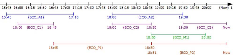
Figure 4 shows a set of (point-based) temporal category occurrences for the Web page category in our running example. Figure 5 shows the corresponding interval-encoded representation (see below for details).
Encoding a set of tuples requires these tuples to be consecutive over the granularity selected. Thus, if the granularity is “minute”, the tuples , and
cannot be included together in the same group, since there is a two-minute gap between them. They must be encoded into two intervals. ∎
| Category | Instance | ||||||||||||||||||||||||||||||||||||||||||||||||||||||||||||||||||||||
| Web Page |
|
Definition 5
[Encoded Category Occurrence] Given a category instance with time granularity G, and a partition of such that the number of sets is minimal. Each set is obtained encoding the occurrences in as in Definition 4, i.e., each contains a set of tuples that can be encoded into a single tuple. Thus, associated to there is a tuple where (a) ID, , …, are the attributes of the occurrences in ; (b) id, , …. are the values for the attributes in (a); (c) is the smallest t of the occurrences in ; (d) is the largest of the occurrences in . We denote an encoded category occurrence (ECO) of the set of occurrences in Given an ECO we denote its associated interval ∎
Example 3
Figure 5 shows a set of eight ECOs encoding the category instance of Figure 4. The Web page with ID=‘P’ (not included in Figure 4) had no filter when it was created until November 29th, 2007 at 18:50, when the attribute filter was updated. Also, the Web page with ID=‘A’ has changed: attribute keyword was updated from ‘Books’ to ‘Computers’, and also filter was updated. Note that there is an interval when this page was not available. After these changes, the page was set off-line at 7:30PM on November 29th, 2007.∎
| [(ID,‘A’), | (catName,‘WebPage’), | (filter,‘’), | (keyword,‘Books’), | [‘11/29/2007 15:45’, ‘11/29/2007 17:10’] ] | |
| [(ID,‘A’), | (catName,‘WebPage’), | (filter,‘P’), | (keyword,‘Computers’), | [‘11/29/2007 18:00’, ‘11/29/2007 19:30’]] | |
| [(ID,‘C’), | (catName,‘WebPage’), | (filter,‘A’), | (keyword,‘Books’), | [‘11/29/2007 16:00’, ‘11/29/2007 16:45’]] | |
| [(ID,‘C’), | (catName,‘WebPage’), | (filter,‘’), | (keyword,‘Games’), | [‘11/29/2007 18:00’, ‘11/29/2007 18:50’]] | |
| [(ID,‘C’), | (catName,‘WebPage’), | (filter,‘M’), | (keyword,‘Games’), | [‘11/29/2007 19:30’, ‘Now’]] | |
| [(ID,‘M’), | (catName,‘WebPage’), | (filter,‘’), | (keyword,‘Games’), | [‘11/29/2007 18:50’, ‘11/29/2007 20:00’]] | |
| [(ID,‘P’), | (catName,‘WebPage’), | (filter,‘’), | (keyword,‘Computers’), | [‘11/29/2007 16:45’, ‘11/29/2007 18:50’]] | |
| [(ID,‘P’), | (catName,‘WebPage’), | (filter,‘A’), | (keyword,‘Computers’), | [‘11/29/2007 18:51’, ‘Now’]] |
Adding a time instant to an ECO, produces an item.
Definition 6 (Item)
Let be an ECO for some category instance. An item I associated to is the set: such that holds. We denote the transaction time of the item.∎
3 A Theory for Support Count
In Section 2 we defined the formal data model we use in the remainder of the paper to build a theory that can help to provide insight into the notion of support. To begin with, over the elements introduced in Definition 1 through 6, we build a simple language, based on sequences of constraints, that we use later to elaborate the concept of support of regular expressions. In short, this language expresses paths of constraints. We define the temporal support of these paths, denoted sequential expressions (SE). SEs are at the cornerstone of our theory. In the next section, we define a regular language that produces SEs, and introduce the notion of temporal support of regular expressions.
Definition 7
[Terms] There exist no others terms than the following ones: (a) Constant: a literal enclosed by simple quotes; (b) Non temporal Attribute: an attribute in the category schema (e.g. filter, url). (c) Temporal Attribute: t, the temporal attribute of and item (see Definition 6); (d) Function of n arguments: Let be a function symbol, the expression is a function where the first parameter is an attribute (temporal or non-temporal), and all the other ones are constants.∎
Definition 8
[Atoms] Let C, A and F be a set of constants, temporal and non temporal attributes and functions, respectively. The expression term1 = term2 is an atom, where term1 A F, term2 C, and is the equality symbol.∎
Definition 9
[Formula] We define recursively a formula by the following rules: (a) An atom is a formula; (b) If F1 and F2 are formulas then F1 F2 is a formula. (c) Nothing else is a formula.∎
Definition 10
[Constraint and Formula of a Constraint] A constraint is a formula enclosed in squared brackets. Given a constraint , we denote the formula of C.∎
Definition 11
[Sequential Expression] A Sequential Expression (SE) of length n is an ordered list of n sub-expressions , where each is a constraint, ∎
Example 4
The sequential expression of length two is composed of two constraints.
We need to define some operations between intervals. Given two intervals and we say that follows if . Saying that an interval follows another interval is equivalent to say that is either after or is met-by in terms of Allen’s Interval Algebra [2].
Example 5
In Figure 5 we can see that Interval() follows
Interval() and Interval(). We can also see that Interval() does not follow
Interval().
Definition 12
[Satisfability of a Constraint] Given a constraint C and an ECO E, we say that E satisfies C if one of the following conditions hold: (a) If is an atom of the form where is an attribute in any of the category occurrences in E, is a constant in and the instantiation of with its value in E, equals . (b) If is an atom of the form where is an attribute in any of the category occurrences in E, is a constant in and the instantiation of in with its value in E, makes the equality true. (c) If is an atom of the form where is a temporal attribute, ‘ct’ is a temporal constant in the temporal domain, with granularity G, and (d) If is an atom of the form where is a temporal attribute, ‘ct’ is a temporal constant in the temporal domain with some granularity G, and the equality is true. (e) If is a formula and and are satisfied by E.
Definition 13
[Satisfability of SE]
Let be a list of ECOs
such that
. We denote a t-ordered list of ECOs.
A sequential expression SE= is satisfied by
if satisfies ,
We denote the set composed of the n lists of ECOs
that satisfy an SE of length . ∎
Example 6
Let us analyze which ordered lists of ECOs in Figure 5 satisfy the SE Here, rollup is the usual rollup function [3], that indicates how a member of an OLAP hierarchy is aggregated. The meaning is that the equality is true when is instantiated with a value that, in the Time dimension, rolls up to the value ‘18’ in the dimension level hour. For example,
The first constraint is satisfied by , , , and . For all of them, there is a time instant within that verifies the rollup predicate. The second constraint is satisfied by and . However, given the temporal order, the only list of ECOs that satisfy the SE is: In (the interval of ) does not follow (the interval of ). ∎
Definition 14
[ToI and Normalized ToI] Let be a finite set of items. A Table Of Items (ToI) for is a table with schema , where Items is the name of an attribute whose instances are items, and an instance of is a finite set of tuples of the form where is an item associated to the object Moreover, given and , two tuples corresponding to the same object, and and the transaction times of the items, then holds. A normalized ToI is a database containing a table with schema (the Normalized ToI), and one table per category, each one with schema ∎
Figure 6 shows an instance of a normalized ToI where items are related to the category instances of Figure 5. There are three sessions (sequences), , and , each one with an associated list of items. The three sessions clicked on URL C, but only would satisfy the constraint (see Figure 5).
| OID | Items | |||||||||
|---|---|---|---|---|---|---|---|---|---|---|
| ||||||||||
| ||||||||||
|
Definition 15
[Temporal Matching of a S.E] Let SE be a sequential expression of length and a normalized ToI (from now on, nToI), with schema An object identified by temporally matches SE, if there exist k tuples in nToI, , where for at least one , , ∎
Example 7
Definition 15 states that if there is a temporally ordered sequence of items such that all of their transaction times fall within the intervals of the ECOs that satisfy the expression, then, we have a temporal match.
With the category occurrences of Figure 5 and the instance of nToI depicted in Figure 6, we analyze the sequential expression SE = The ECOs that satisfy the first constraint are and . The second constraint is satisfied by . Thus, the lists that satisfy SE are and . The object temporally matches SE, since there exist two different tuples in whose transaction times belong to and , respectively. With a similar analysis, does not match the SE. The ECO did not exist when the user in this session clicked the last two URLs. Finally, temporally matches SE, because the transaction time of belongs to the interval of and the transaction time of belongs to the interval of Intuitively, this means that the user of could have chosen the URL with ID=‘P’, which existed at the time she chose the URL with ID=‘M’.∎
From Definition 15, it follows that if a list of ECOs does not satisfy a sequential expression SE, no object in the nToI can use this list to temporally match SE. Thus, given that the lists in are computed over the category occurrences, which usually fit in main memory, unnecessary database scans can be avoided.
Definition 16
[Temporal Satisfability of a Constraint] Given a constraint C and a normalized ToI, with schema we say that a tuple in nToI temporally satisfies C if at least one of the following conditions hold: (a) if is an atom of the form where is a term for temporal attributes of items, ‘ct’ is a temporal constant in the temporal domain with some granularity and ; (b) if is an atom of the form where is a temporal attribute, ‘ct’ is a temporal constant, and ; (c) if does not contain a temporal attribute; (d) if is a formula and F1 and F2 are satisfied by .∎
Definition 17
[Total Matching of a Sequential Expression] Given a sequential expression SE=.… of length k, and a normalized ToI with schema we say that an object identified by totally matches SE, if there exists different tuples in nToI, of the form ,…,, and there is at least one list where the following conditions hold: (a) (b) is the identifier of the encoded category occurrence (c) is temporally satisfied by We denote each a list of interest for SE.∎
Property 1
Given a sequential expression SE=.… of length k, and a normalized ToI with schema If an object in does not temporally match SE, then cannot totally match SE.∎
Property 2
Given a sequential expression SE=.… of length k, and a normalized ToI with schema such that there is an object in that totally matches SE, then temporally matches SE. ∎
Example 8
Object in Example 7, totally matches SE, using the second and third tuples, together with list . On the other hand, does not totally match SE, since it does not temporally match the expression. Finally, temporally matches SE, but it does not totally match it, because does not satisfy the second condition in Definition 17.∎
Definition 18 (Temporal Support of SE)
The temporal support of a sequential expression SE, denoted is the quotient between the number of different objects that totally match SE and the number of different objects that temporally match SE, if the latter is different to zero. Otherwise . ∎
Definition 18 formalizes the intuition behind the concept of temporal support, namely, counting only the sequences that could have potentially generated a matching sequence, given the temporal availability of the category occurrences to which an item in a sequence belong (these sequences are the ones that temporally match a SE). Classic support count, instead, considers the whole number of sequences in the database.
Example 9
In the example above The object is not considered in the support count because when the user clicked the Web page, it had not the possibility of selecting pages that satisfy the constraint. ∎
4 Temporal Support of Regular Expressions
Having defined the temporal support of a sequential expression, we now move on to the general problem, i.e., defining the same concept for an RE. The data model defined in Section 2, and the theory developed in Section 3, allows us to define a language based on RE over constraints, that supports categorical attributes. We start with a simple example. We wish to restrict the result of an SPM algorithm to the sequences that match the following expressions: (a) =[keyword=‘Games’]; (b) = [keyword=‘Games’].[filter=‘’]; (c) = [keyword=‘Games’].[filter=‘’].[filter=‘’]. For each , a condition [filter=‘’] is added. We are also interested in computing the temporal support of these sequential expressions. Instead of computing each support in a separate fashion, we may want to summarize these sequences in a single RE, namely: .
Definition 19
[R.E. over constraints] A regular expression over the constraints of Definition 10, is an expression generated by the grammar
where is a constraint, is the symbol representing the empty expression, means disjunction, means concatenation, “zero or one occurrence”, “one or more occurrences”, and “zero or more occurrences”. The precedence is the usual one.∎
Property 3
Let be the set of sequential expressions produced by a RE generated by the grammar of Definition 19. There is also a normalized ToI with schema If an object in the nToI temporally or totally matches any SE in matches , temporally or totally, respectively. ∎
Property 3 follows from observing that [keyword=‘Games’].[filter=‘’]* could be written: [keyword=‘Games’] ([keyword=‘Games’].[filter=‘’]) ([keyword= ‘Games’].[filter=‘’].[filter=‘’]) ([keyword=‘Games’].[filter=‘’].[filter=‘’].[filter=‘’])
Reasoning along the same lines, since a regular expression over an alphabet (in our case, constraints) denotes the language that is recognized by a Deterministic Finite Automata (DFA), there exists a (possible infinite) set of strings over the alphabet that this DFA accepts. Each of these strings (actually, strings composed of constraints) matches our definition of SE. Then, we extend our previous definition of temporal and total matching of SE, to RE, as follows.
Definition 20 (Temporal Matching of a RE)
Given a regular expression generated by the grammar of Definition 19, and the DFA that accepts There is also a normalized ToI with schema We say that temporally matches if there exists some such that there exists at least one string of length accepted by and temporally matches this string. ∎
Definition 21 (Total Matching of a RE)
Given a regular expression generated by the grammar of Definition 19, and the DFA that accepts There is also a normalized ToI with schema We say that totally matches RE, if there exists some such that there is at least one string of length n accepted by and totally matches this string. ∎
Definition 22 (Temporal Support of a RE)
The temporal support of a regular expression denoted is the quotient between the number of different objects that totally match and the number of different objects that temporally match , if the latter is different to zero. Otherwise . ∎
We use the example above to show how sequential expressions are summarized using the language of Definition 19. We use the category occurrences and the nToI shown in Figures 5 and 6, respectively. We first apply Definition 12 in order to check satisfability of the constraints in the expressions through ECOs , and from Figure 5 satisfy the constraint [keyword=‘Games’]. Analogously, the constraint [filter=‘’] is satisfied by , , and . Next, for each SE, we check satisfability applying Definition 13. For =[keyword=‘Games’] we obtain , . For =[keyword=‘Games’].[filter=‘’] we have , Note that, for example, the list does not satisfy because follows . For = [keyword=‘Games’].[filter=‘’].[filter=‘’], we have , , , , . Also here, many lists are discarded. For instance, does not satisfy because follows .
Now, we can compute the temporal support of each SE, applying Definitions 15 through 18. For from the third tuple in and we conclude that totally (and hence, temporally) matches . From the first tuple in and totally matches . From the first or third tuples in and totally matches . Finally, the temporal support of is
In a similar way, we can conclude that the support of and are, respectively, and Since no session has four tuples, it is not necessary to analyze a sequential expression of length four, like for instance [keyword=‘Games’].[filter=‘’].[filter=‘’].[filter=‘’].
5 Future Work
We expect to extend our work in two ways. On the one hand, the theoretical framework introduced here allows to think in a more general definition of support, with different semantics (not only temporal), that may enhance current data mining tools. On the other hand, we will develop an optimized implementation of the algorithm that can support massive amounts of data.
References
- [1] R. Agrawal and R. Srikant. Mining sequential patterns. In Proc. of the Int’l Conference on Data Engineering (ICDE), 1995.
- [2] James F. Allen. Maintaining knowledge about temporal intervals. Commun. ACM, 26(11):832–843, 1983.
- [3] L. Cabibbo and R. Torlone. Querying multidimensional databases. In Proceedings DBPL’97, pages 253–269, East Park, Colorado, USA, 1997.
- [4] M. N. Garofalakis, R. Rastogi, and K. Shim. Spirit: Sequential pattern mining with regular expression constraints. In Proceedings of the 25th VLDB Conference, 1999.
- [5] M. N. Garofalakis, R. Rastogi, and K. Shim. Mining sequential patterns with regular expression constraints. In IEEE Transactions on Knowledge and Data Engineering, 2002.
- [6] J. Huang, C. Tseng, J. Ou, and M. Chen. A general model for sequential pattern mining with a progressive database. IEEE Transactions on Knowledge and Data Engineering, 20(9):1153–1167, 2008.
- [7] C. Lee, C. Lin, and M. Chen. On mining general temporal association rules in a publication database. In ICDM, pages 337–344, 2001.
- [8] Y. Li, P. Ning, X.S. Wang, and S. Jajodia. Discovering calendar-based temporal association rules. Data Knowl. Eng., 44(2):193–218, 2003.
- [9] F. Masseglia, P. Poncelet, and M. Teisseire. Incremental mining of sequential patterns in large databases. Data Knowl. Eng., 46(1):97–121, 2003.
- [10] A. Ntoulas, J. Cho, and C. Olston. What’s new on the web?: the evolution of the web from a search engine perspective. In WWW ’04, pages 1–12, New York, NY, USA, 2004. ACM.
- [11] S. Parthasarathy, M. J. Zaki, M. Ogihara, and S. Dwarkadas. Incremental and interactive sequence mining. In CIKM ’99, pages 251–258, New York, NY, USA, 1999. ACM.
- [12] R. Srikant and R. Agrawal. Mining sequential patterns: Generalizations and performance improvements. In Proc. of the Fifth Int’l Conference on Extending Database Technology (EDBT), 1996.
- [13] A. Tansel, J. Clifford, and S. Gadia (eds.). Temporal Databases: Theory, Design and Implementation. Benjamin/Cummings, 1993.
- [14] Abdullah Uz Tansel and Susan P. Imberman. Discovery of association rules in temporal databases. In ITNG, pages 371–376, 2007.
- [15] David Toman. Point vs. interval-based query languages for temporal databases. In PODS, pages 58–67, 1996.
- [16] I. H. Toroslu and M. Kantarcioglu. Mining cyclically repeated patterns. In DaWaK ’01, pages 83–92, London, UK, 2001. Springer-Verlag.