Characterising the Gravitational Instability in Cooling Accretion Discs
Abstract
In this paper we perform a systematic analysis of the structure induced by the onset of gravitational instabilities in cooling gaseous accretion discs. It is well known that for low enough cooling rates the disc reaches a quasi-steady configuration, with the instability saturating at a finite amplitude such that the disc is kept close to marginal stability. We analyse the dependence of the saturation amplitude on the imposed cooling rate, and we find that it scales with the inverse square root of the cooling parameter . This indicates that the heating rate induced by the instability is proportional to the energy density of the density waves excited by the disc self-gravity. In particular, we find that at saturation the energy dissipated per dynamical time by weak shocks due to the gravitational perturbations is of the order of 20 per cent of the wave energy. We further perform a Fourier analysis of the disc structure, and subsequently determine the dominant radial and azimuthal wavenumbers of the density waves. While the number of spiral arms (corresponding to the azimuthal wavenumber) is fairly constant with radius, we find that the disc displays a range of radial wavenumbers whose mean increases with increasing radius. The dominant modes closely match the locally most unstable wavelength as predicted by linear perturbation analysis. As a consequence, we demonstrate numerically that the density waves excited in relatively low mass discs are always close to co-rotation, deviating from it by approximately 10 per cent. This result can be understood in terms of the constancy of the Doppler-shifted phase Mach number of the flow – the pattern speed self-adjusts so that the flow into spiral arms is always sonic. This has profound effects on the degree to which the extraction of energy and angular momentum from the mean flow through density waves can be modelled as a viscous process. Our results thus provide (a) a detailed description of how the self-regulation mechanism is established for low cooling rates, (b) a clarification of the conditions required for describing the transport induced by self-gravity through an effective viscosity, (c) an estimate of the maximum amplitude of the density perturbation before fragmentation takes place, and finally (d) a simple recipe to estimate the density perturbation in different thermal regimes.
Keywords:
accretion, accretion discs – galaxies: active – gravitation – hydrodynamics – instabilities – planetary systems: formation1 Introduction
In cold, relatively massive accretion discs the effects of the disc self-gravity can become dynamically important, and gravitational instabilities may play a major role in determining the long-term evolution of the disc. On the one hand the instability can induce fragmentation of the disc, potentially resulting in the formation of massive stars in AGN accretion discs (Nayakshin et al., 2007) or, in the case of proto-planetary discs, low-mass companions (Stamatellos et al., 2007) or even giant planets (Boss, 1997; Boss, 1998). On the other hand, the instability is very effective in transporting and redistributing angular momentum within the disc (Lodato & Rice, 2004; Lodato & Rice, 2005) and might therefore promote accretion in a variety of different contexts and scales, from supermassive black hole growth (Shlosman et al., 1990; Lodato & Natarajan, 2006) to star formation (Vorobyov & Basu, 2005).
The balance between the heating provided through such gravitational instabilities and the cooling as energy is radiated away is known to have major implications for the fate of the disc. Fragmentation into bound objects occurs when the cooling dominates, whereas the disc can persist in a quasi-equilibrium marginally stable condition if the cooling rate is sufficiently low (Gammie, 2001; Rice et al., 2005; Lodato & Rice, 2004).
Such a quasi-steady state is characterised by the presence of spiral density waves, which transport energy and angular momentum through the disc. Where the discs are weakly ionised, and therefore where the magneto-rotational instability is likely to be ineffective, this angular momentum transport mechanism may be the primary driver of accretion. Additionally, these waves extract rotational energy from the disc, some of which is then returned as heat as the waves steepen into shocks. This heat then stabilises the disc against further gravitational collapse into bound fragments. As the amplitude of the waves increases, so too does the wave energy density, increasing the reservoir of energy available to be returned to the disc as heat. However, numerical experiments (Gammie, 2001; Rice et al., 2005) have shown that if the cooling time is less than a few times the local dynamical time , this feedback process breaks down and fragmentation ensues. The quasi-steady marginal stability state therefore represents a restricted regime of dynamic thermal equilibrium, where the heating through gravitational instabilities is balanced by the cooling rate.
In this paper we seek to characterise the relationship between the strength of the cooling and the amplitude of the spiral density waves excited within the disc through self-gravity, while remaining within this dynamic thermal equilibrium state. To this end we use a Smoothed Particle Hydrodynamics (SPH) code to run global numerical simulations of self-gravitating gaseous discs. From such controlled numerical experiments, we measure the amplitude of the density perturbations over a range of cooling times, down to the limit where the disc fragments, and to investigate the overall structure formation. Fourier analysis allows us to characterise the mode spectra and pattern speeds associated with this structure, and to associate the dynamics of the spiral density waves excited through self-gravity with the thermodynamics of the disc self-regulation process. We begin by discussing some relevant properties of density waves and transport processes in gaseous discs in Section 2, and link this to the disc thermodynamics in Section 3. Details of the numerical simulations and initial conditions are given in Section 4, and the results of these simulations are presented in Section 5. In Section 6 we discuss the implications of these results and the conclusions that may be drawn from them.
2 Dynamics of Self-Gravitating Gaseous Discs
In the following two sections we derive analytically the basic relations that link the disc quantities in the presence of perturbations to the induced transport properties of self-gravitating discs. These standard results have been mostly derived in the context of stellar dynamics (Shu, 1970; Bertin, 2000; Binney & Tremaine, 2008). In the context of gaseous (accretion) discs, qualitatively similar (but rather more involved) analyses have been presented in Balbus & Papaloizou (1999) and Balbus (2003).
2.1 Dispersion Relations for Self-Gravitating Discs
The linear development of the gravitational instability is usually described by the dispersion relation between the wave (angular) frequency and the radial and azimuthal wavenumbers of excited modes, and respectively. For an infinitesimally thin (i.e. 2-dimensional) disc, this can be obtained using the standard WKB method of perturbation analysis, and in the tight-winding limit (where the radial wavelength is small in comparison to the azimuthal wavelength, , with the cylindrical radius) we have
| (1) |
where is the angular speed, and is the epicyclic frequency, is the sound speed and is the surface density of the umperturbed disc (Binney & Tremaine, 2008). Introducing the pattern speed of the wave , where , we may express this as follows;
| (2) |
The well known stability criterion for axisymmetric disturbances (Toomre, 1964)
| (3) |
identifies the region of parameter space where the RHS of Eq.(2) is positive definite, and therefore where the disc is stable at all wavelengths. For the case of an unstable disc, the most unstable wavelength (i.e. where the RHS of Eq.(2) is at a minimum) occurs at a radial wave-number
| (4) |
For a marginally stable disc where we would therefore expect only modes with to be excited, and in this instance, Eq.(2) tells that , i.e. all excited modes are expected to be close to co-rotation. Note that the most unstable wave-number is exactly the inverse of the disc thickness for a self-gravitating disc
| (5) |
where the last approximation is exact for a Keplerian rotation curve.
2.2 The Stress Tensor
In non-axisymmetric self-gravitating discs, torques arising due to the perturbed gravitational potential play an important role in transporting both energy and angular momentum.
Traditionally, viscous accretion discs are described by the -formalism of Shakura & Sunyaev (1973), where (for an infinitesimally thin disc) the only non-vanishing component of the vertically integrated stress tensor is the shear term, defined as
| (6) |
where is a dimensionless parameter which measures the viscosity. In this case the disc stress is linked to the local pressure , and indicates that the -formalism is fundamentally a local relationship. Furthermore, since is not necessarily constant, this represents a completely general description for any purely local process. Also note that for Keplerian rotation, , implying that the stress is negative, i.e. it acts to oppose rotation, and therefore allows for inward accretion flows.
Accretion disc theory identifies the origin of the stress with torques arising due to perturbations in a “turbulent” disc. Crucially for the gas dynamics, these perturbations manifest themselves as fluctuations in the mean flow velocity, the gravitational potential and the magnetic field threading the disc. For non-magnetised self-gravitating discs such as we consider here, the stress tensor can therefore be broken down into a Reynolds stress term, associated with velocity fluctuations, and a gravitational stress term, associated with fluctuations in the gravitational potential. The Reynolds stress term is such that
| (7) |
(where are the velocity fluctuations about the mean flow velocity in the and directions respectively and the brackets indicate azimuthal averaging) and the gravitational stress term is given by Lynden-Bell & Kalnajs (1972) as
| (8) |
where again the are the accelerations due to the perturbed gravitational potential of the disc in the and directions respectively.
The viscous torque per unit area is related to the vertically integrated stress tensor through
| (9) |
which in turn yields
| (10) |
as the only non-zero component of the torque. The power per unit surface produced by this viscous torque is then given simply by (Frank et al., 2002; Pringle, 1981)
| (11) |
where the subscript indicates that this relation is expected for a viscous disc. Equation (11) therefore links the transport of angular momentum and the associated rate of work done by torques in the case of a local process, as historically modelled via the -viscosity parameter.
2.3 Wave Energy and Angular Momentum Densities
In this section we turn our attention to the transport of energy and angular momentum through the propagation of the spiral density waves expected to arise in a self-gravitating disc. To this end it is convenient to introduce the wave action density for density waves. Within the WKB approximation used to derive the dispersion relation given in Eq.(2), the wave action per unit surface is given by (Toomre, 1969; Shu, 1970; Fan & Lou, 1999)
| (12) |
where is the perturbed gravitational potential, itself given by
| (13) |
where is the surface density perturbation. The wave energy per unit surface and the wave angular momentum per unit surface are obtained in a straightforward way from the wave action through the standard wave dynamics relations (Bertin, 2000; Shu, 1970), 11 1 Note that this system of equations is analogous to that found in quantum mechanics for an harmonic oscillator; from the quantum of action , the quantized energy and angular momentum are found via and , where and are the angular frequency and spin quantum number respectively.
| (14) |
| (15) |
Combining the first of these relations with Eqs.(12) and (13) we obtain
| (16) |
where
| (17) |
| (18) |
are the radial phase speed and Doppler-shifted radial phase speed of the wave respectively. Note that Eqs.(16) and (18) together explain why self-induced density waves are launched at co-rotation – since the energy density changes sign at co-rotation, waves that propagate away from co-rotation extract no net energy from the flow.
Looking again at Eqs.(14) and (15), we see that the relationship between the energy per unit surface and the angular momentum per unit surface in a density wave is given by
| (19) |
In the case of quasi-stationary waves (where is constant) propagating in a disc in dynamic thermal equilibrium, the rate at which energy is lost per unit surface due to cooling must be balanced by the power per unit surface dissipated by the waves. In order to maintain the amplitude of the wave, the instability has to keep extracting energy and angular momentum from the background flow. The fluxes of energy (angular momentum) carried by the wave are simply () times the local group velocity. Hence when a wave dissipates it adds energy and angular momentum to the flow in the ratio of to , i.e. in the ratio . We therefore conclude that
| (20) |
Equation (20) is the wave analogue of Eq.(11). Comparing these two equations, we note a fundamental difference with respect to the viscous model – for a given torque , waves extract energy from the flow at a rate proportional to the wave pattern speed , whereas the rotation speed is the underlying rate in the local (viscous) case.
Balbus & Papaloizou (1999) have noted similarly that in general, energy transport through the gravitational instability cannot be described purely in viscous terms, and indeed this is only possible at co-rotation, when . This can be readily understood if we consider that the wave energy per unit surface (Eq.(16)) can be decomposed into two separate terms, as follows;
| (21) |
The second term, equal to the angular momentum per unit surface times the rotation speed , is a local energy transport term (cf. Eq.(11)) and can therefore be represented using the -formalism. The first term however, equal to the same angular momentum term times , is a non local term. In fact the energy flux associated with this non-local transport term is is precisely that identified by Balbus & Papaloizou (1999) as an “anomalous flux”, preventing self-gravitating discs from acting as pure -discs.
We see that far from co-rotation, where , this term becomes significant, and thus non-local (global) transport becomes important within the disc. For trailing waves launched at co-rotation, the direction of energy (and angular momentum) transport is outwards throughout the disc (i.e. inward travelling waves with negative energy density inside co-rotation and outward travelling waves with positive energy density outside co-rotation), and thus the dissipation of such waves effects a net outward transport of energy (and angular momentum). If such a wave dissipates at large radius (where ) then the ratio in which energy and angular momentum are added to the disc (Eq.(20)) is significantly greater than the equivalent ratio in the viscous case (Eq.(11)). Consequently, under such conditions the energy dissipated at large radii in a steady state disc with wave transport can significantly exceed that dissipated in an equivalent viscous disc – with this extra energy being extracted by the wave from deep in the potential and transported to large radii (Lodato & Bertin, 2001; Bertin & Lodato, 2001). However, if waves instead dissipate close to co-rotation, the wave transport is dominated by the local term in Eq.(21); since energy and angular momentum transport are exchanged with the disc in roughly the same ratio as for a viscous process, then in this regime the -formalism is a good approximation to the actual transport properties of the disc.
From Eq.(21) it is therefore possible to quantify a non-local transport fraction , from the ratio of the two terms on the RHS, such that
| (22) |
Thus in order to assess the importance of non-local effects, we need to know the relationship between the angular frequency and the pattern speed . In section 5.5 we use the dispersion relation along with information extracted through Fourier analysis in order to estimate the pattern speed, and hence to evaluate directly.
3 Simulating the Disc Thermodynamics
Realistically simulating the thermodynamics of accretion discs is a complex undertaking and as such has received much attention, from the opacity-based treatment employed by Johnson & Gammie (2003) through to the various convective and radiative transfer models of Boss (2004), Boley et al. (2007), Mayer et al. (2007), Stamatellos & Whitworth (2008a) and Stamatellos & Whitworth (2008b), the latter two of which also account for heating from the central star.
However, in this paper, one of our aims is to investigate the relationship between the properties of the density perturbations and the rate at which the disc cools. This purpose is served most readily by imposing a known cooling rate against which the heating rate and subsequent disc structure may be easily correlated. It is therefore not necessary to consider the exact physics of the cooling regimes found in astrophysical discs, and hence we can use a cooling law for the heat loss rate per unit mass , such that
| (23) |
where is the internal energy per unit mass and where the details of the cooling function (and possibly of additional external heating) are absorbed into the simple parameter . As long as such a characteristic timescale can be defined, it is therefore possible to use this formalism to represent a wide range of cooling mechanisms. Within this paper, we use a fixed ratio between the local dynamical and cooling timescales, such that is constant. This form of cooling has been used extensively in simulations of discs in various contexts, for example Gammie (2001), Lodato & Rice (2005), Hobbs & Nayakshin (2008), and has proven useful in elucidating the properties of the gravitational instability in controlled numerical experiments.
In terms of the heating from the gravitational instability, we noted in the previous section that density waves extract energy from the disc. In addition to compression heating, in the case where the pattern speed differs from the rotation speed by more than the local sound speed, these waves will steepen into shocks, liberating further heat into the disc. We expect the rate at which energy is added to the disc to scale with the energy of the wave and the local dynamical timescale, and we can then express the heating rate per unit mass due to the instability as
| (24) |
where we define the radial phase and Doppler shifted phase Mach numbers to be and respectively. In Eq. (24) we have also introduced a dimensionless proportionality factor , hereinafter referred to as the heating factor. If the relationship between the pattern speed and the angular speed is self-similar (i.e., it does not vary across the disc), we expect to be simply a constant, independent of radius.
Once the gravitational instability has been instigated and has subsequently saturated, we may consider the disc to be in dynamic thermal equilibrium, such that the energy released through wave-driven shock and compression heating is balanced by the imposed cooling, i.e. . Recalling that , we can equate equations (24) and (23) and thereby determine the following relationship between the amplitude of the density perturbations and strength of the cooling, as measured by the parameter;
| (25) |
In this paper we shall therefore use global numerical simulations to test the above energy balance, and to investigate the relative magnitude of the local and and non-local transport terms.
4 Numerical Set-Up
4.1 The SPH code
All of the simulations presented hereafter were performed using a 3D smoothed particle hydrodynamics (SPH) code, a Lagrangian hydrodynamics code capable of modelling self-gravity (see for example, Benz 1990; Monaghan 1992). All particles evolve according to individual time-steps governed by the Courant condition, a force condition (Monaghan, 1992) and an integrator limit (Bate et al., 1995).
We note here that with SPH, the integral of a physical quantity over a given volume is estimated by the sum over the individual particle values of this quantity, as below;
| (26) |
where is the particle mass, and loops over all the particles within the volume . In a similar manner, we note that a volume-averaged value for , which we shall call , can therefore be estimated via
| (27) |
when, as in all our simulations, all particles have the same mass.
We have modelled our disc systems as a single point mass (onto which gas particles may accrete if they enter within a given sink radius, and satisfy certain boundness conditions – see Bate et al. 1995) orbited by 500,000 SPH gas particles; a set up common to many other SPH simulations of such systems, (e.g. Lodato & Rice 2004; Lodato & Rice 2005; Rice et al. 2003; Clarke et al. 2007) but with increaesd resolution. The central object is free to move under the gravitational influence of the disc. In order to ensure the simulations were properly converged, resolution checks were undertaken with discs consisting of both 250,000 and 1,000,000 particles – these are discussed briefly in Appendix A.
As described in section 3 we use a simple cooling model, implemented in the following manner
| (28) |
where the and are the internal energy per unit mass and the cooling time associated with each particle respectively. Again as above the functional form of the cooling time is kept simple, such that , where is the angular velocity of each particle, and where is held constant throughout any particular simulation. All simulations have been run modelling the particles as a perfect gas, with the ratio of specific heats , heat addition being allowed for via work and shock heating and with the cooling implemented as specified above. Artificial viscosity has been included through the standard SPH formalism, with and . Note that these values are smaller than those commonly used in SPH simulations; we use these values to limit the transport induced by artificial viscosity. As shown in Lodato & Rice (2004), with this choice of parameters the transport of energy and angular momentum due to artificial viscosity is a factor of 10 smaller than that due to gravitational perturbations, while we are still able to resolve the weak shocks occurring in our simulations.
By using the cooling prescription outlined above, the rate at which the disc cools is governed by the dimensionless parameter and the cooling is thus implemented scale free. The governing equations of the entire simulation can likewise be recast in dimensionless form. In common with the previous SPH simulations mentioned above, we define the unit mass to be that of the central object – the total disc mass and individual particle masses are therefore expressed as fractions of the central object mass. We can self-consistently define an arbitrary unit (cylindrical) radius , and thus, with , the unit time is the dynamical time at radius .
| No. of Particles | Duration | ||
| 4 | 0.10 | 500,000 | 4.0 |
| 5 | 0.10 | 500,000 | 10.0 |
| 6 | 0.10 | 500,000 | 10.0 |
| 7 | 0.10 | 500,000 | 10.0 |
| 8 | 0.10 | 500,000 | 10.0 |
| 9 | 0.10 | 500,000 | 10.0 |
| 10 | 0.10 | 500,000 | 10.0 |
| 5 | 0.050 | 500,000 | 10.0 |
| 5 | 0.075 | 500,000 | 10.0 |
| 5 | 0.100 | 500,000 | 10.0 |
| 5 | 0.125 | 500,000 | 10.0 |


4.2 Initial conditions
All our simulations model a central point object of unit mass , surrounded by a gaseous disc of mass . Although the bulk of the simulations have been conducted with a disc to central object mass ratio of 0.1, simulations have been run with and to investigate the effects of the mass ratio on the non-local energy transport fraction .


All simulations have used an initial mass surface density profile , which implies that in the marginally stable state where , the disc temperature profile should be approximately flat. Since the surface density evolves on the viscous time this profile remains roughly unchanged throughout the simulations. The initial temperature profile is and is such that the minimum value of the Toomre parameter occurs at the outer edge of the disc. In this manner the disc is initially gravitationally stable throughout. Note that the disc is not initially in thermal equilibrium – heat is not input to the disc until gravitational instabilities are initiated.
Radially the disc extends from to , as measured in the code units described above. The disc is initially in approximate hydrostatic equilibrium in a Gaussian distribution of particles with scale height . The azimuthal velocities take into account both a pressure correction (Lodato, 2007) and the enclosed disc mass. In both cases, any variation from dynamical equilibrium is washed out on the dynamical timescale.
Given the dimensions above, one outer dynamical timescale of the disc corresponds to 125 time units. To ensure that thermal equilibrium is reached and that the gravitational instability is saturated, all simulations are followed for at least 10 outer cooling times. To this end we shall refer to the thermal time for each simulation as the cooling time evaluated at the initial outer edge of disc, taken to be at – thus .
4.3 Simulations run
In all a total of nine distinct simulations were run for various values of the cooling parameter and the disc to central object mass ratio , as detailed in Table 1. Although previous investigations with have found that the fragmentation boundary is at , (Rice et al., 2005; Rice et al., 2003), we find that in the case where the fragmentation boundary is slightly different, with . The simulation where therefore contains a fragment, and is included primarily for completeness. All results henceforth are given at the time quoted in the final column of Table 1 unless otherwise stated. The raw data are time-averaged over 500 unit times about these values to enhance the signal-to-noise ratio and to give the approximate steady-state values.
5 Simulation Results
Common to all the simulations run is an initial phase in which the discs cool rapidly until the value of becomes approximately unity, at which point the gravitational instability is initiated and heat is liberated to balance the cooling. This stage is complete after approximately one thermal time, and from then on the discs settle into a quasi-steady state characterised by the presence of spiral arms throughout almost their entire radial range, with . The quasi-static profiles to which the discs converge are shown in Fig. 1, with the cooling parameter varying in the top panel, and the disc to central object mass ratio varying in the bottom panel. Note that the data are plotted at the times given in Table 1. Throughout all the simulations it can be seen that the discs self-regulate to the marginally stable condition over a large range of radii.
Once the disc has reached a quasi-steady state, the disc aspect ratio also stabilises to the value predicted by the self-regulation condition :
| (29) |
and is shown as a function of radius in Fig. 2 for different values of (top panel) and (bottom panel).
5.1 Saturation amplitude of the instability
Once the gravitational instability has been initiated, for the case where (i.e. where ) the amplitude of the perturbations required to balance the cooling rises to the point where non-linear effects dominate, leading to the fragmentation of the disc into bound objects. In the case where however, the amplitude increases on the dynamical timescale until the disc reaches dynamic thermal equilibrium, at which point the amplitude of the surface density fluctuations becomes constant, and the heating they provide balances the imposed cooling. This is observed in all our simulations where .
From the simulations we can now test the prediction for the saturation amplitude provided by Eq.(25) numerically. Fig. 3 shows images of the surface density of the disc for the two cases and , respectively, where in both cases the mass ratio is . It can be seen that, while the overall disc structure remains essentially constant (as confirmed by a more detailed Fourier analysis, see below), the spiral wave amplitude as characterised by the surface density contrasts appears to decrease with increasing . Noting that the direction of rotation of the discs is anticlockwise, we find that throughout our simulations the waves excited are all trailing waves – they all point in opposition to the direction of rotation.
While the SPH code allows us to conduct a global 3D simulation of discs with relative ease, it does not permit the direct calculation of an intrinsically 2D quantity, such as the surface density perturbation amplitude . Therefore, in order to calculate this quantity, we overlay a cylindrical grid on the disc, such that each cell contains approximately particles, where is the average number of neighbours within a smoothing kernel for our simulations. For each annulus of cells we can calculate an average surface density , and by comparing this to the value calculated for each cell within this annulus we can evaluate an annulus averaged RMS value for the perturbation amplitude . This is shown as a function of radius and the cooling parameter in Fig. 4.


From Fig. 4, it is clear that there is an increasing trend in with decreasing and that furthermore, away from the disc boundaries the saturation amplitude is approximately constant with radius. The low values for the perturbation amplitude at small radii () are probably due to the increased number of particles per grid cell smoothing out the underlying variation. We can however characterise the strength of the perturbation by simply averaging over the self-regulated portion of the disc, that we define as (cf. Fig 1). Fig. 5 shows the relation between the azimuthally and radially averaged amplitude, which we denote as , and the cooling parameter . Each point represents a single simulation, while the curve shows our best fit to the data using the inverse square root dependence predicted by Eq.(25). From the simulations we therefore obtain the following empirical relationship, for the case where
| (30) |

In a similar manner we can also calculate the variation in with , which is shown in Fig. 6. We see that the strength of the perturbation tends to increase with the mass ratio , although it is clear that this dependence on is rather less than linear.
5.2 Fourier analysis: azimuthal structure
From the simulations we have found empirically that the perturbation strength follows a relationship, as predicted by Eq.(25). However, this equation also shows a clear dependence on the wave modes excited within the disc through the action of the gravitational instability. To elucidate this relationship further we have therefore conducted a Fourier analysis of the wave modes in the disc, a full description of which may be found in Appendix B. In this section we therefore consider the effects of both the cooling (via ) and the disc to central object mass ratio on the excitation of the azimuthal wavenumbers – the next section will describe the excitation of the radial wavenumbers.


We find that in general, whatever the imposed cooling regime, for a given mass ratio the distribution of the azimuthal wavenumbers determined by the gravitational instability remains approximately constant, with the dominant mode at around . The mode distributions at five radii throughout the disc for the cases where and are shown in Fig. 7. It is clear that the spectral distribution of the modes shows little variation with radius and with the imposed cooling, except that the amplitude of the modes decreases as increases, as expected in view of the decreased perturbation amplitudes seen in Figs 3, 4 and 5. Additionally, Fig. 8 (top panel) shows the variation of the average wavenumber against radius for all the values of that have been tested, and we note that although some small variation is seen, it is uncorrelated with the imposed cooling.
The bottom panel of Fig. 8 shows the variation in the average azimuthal modes excited as the disc to central object mass ratio varies, while the cooling is held constant with . It can be seen from the plot that variation of this parameter does have a marked effect on the power spectrum of the waves – the average mode number varies inversely with the mass ratio, from where to where . This variation is also clearly seen in Fig. 9, where a large number of flocculent arms are present in the disc with , and fewer, rather more well-defined spiral arms appear in the disc where (cf. the similar result obtained in Lodato & Rice 2004). By comparison, the left panel of Fig. 3 shows a disc with and , and the pattern of spiral arms present is intermediate to those shown in Fig. 9.
5.3 Fourier analysis: radial structure
We now consider the radial wavenumbers of the waves excited by the gravitational instability. In contrast to the azimuthal modes, it is clear from Figs. 3 and 9 that there is significant variation in the radial wavenumber with radius, and Fig. 9 suggests that there is an additional variation with the disc to central object mass ratio.
In Fig. 10 we show the variation in the power spectrum of different radial wavenumbers for the cases where and and , at the same radii as the azimuthal wavenumbers shown in Fig. 7. As with the azimuthal modes, we see little overall change in the spectral distribution of the modes with varying excepting that the amplitudes of the modes decrease as the cooling weakens. Conversely however, these plots show a significant variation with radius, in that the peak wavenumber decreases with increasing radius, and thus the dominant wavelength similarly increases with radius.
Figure 11 on the other hand shows the power spectrum as a function of , where we normalize the wavenumber to the expected most unstable one, (see Section 2.1). We thus confirm the expectations from the linear WKB approach, as these plots show a clear peak at . This therefore suggests that throughout the disc the excited waves are close to co-rotation. Fig. 12 (top panel) shows the average radial wavenumber as a function of radius for all the values of considered, again confirming the trends already discussed and also further showing that, excepting the variation in amplitude discussed above, the structure excited by the simulation is essentially independent of the cooling imposed. It also shows that the simulation to simulation scatter is very small.
The bottom panel of Fig. 12 shows that, as with the azimuthal wavenumbers, there is clear variation in the average radial wavenumber with the disc to central object mass ratio for a given (in this case ); increasing the mass ratio decreases the average wavenumber in approximate inverse proportion. The dashed line in the bottom panel of Fig. 12 plots a simple curve, indicating that the average wavenumber follows a power-law distribution with radius, such that , which remains constant with varying mass ratio. This is easily understood by noting that since the sound speed is approximately constant by construction, Eq.(4) indicates that .

5.4 Mach number of the spiral modes
Returning briefly to the dispersion relation given in Eqs.(1) and (2), we note that this is only strictly valid for infinitesimally thin discs. As our simulations are fully three dimensional, we require a correction to the self-gravity term to account for this, and this is shown in Eq.(31) below (Bertin, 2000),
| (31) |
where we have also used the fact that our discs are approximately Keplerian, and thus . The reduction factor of arises from the vertical dilution of the gravitational potential due to the finite thickness of the disc (Bertin, 2000; Binney & Tremaine, 2008; Vandervoort, 1970). Using this finite-thickness dispersion relation and our averaged values for and it is possible to calculate a Doppler-shifted angular speed , noting that the sign of cannot be determined from Eq.(31). Since the average radial wave-number is always very close to the most unstable one, and since the disc is almost exactly marginally stable, the resultant average pattern speed turns out to be always very close to co-rotation (as can be seen in Fig. 16). We quantify the deviation of the pattern speed from co-rotation later in section 5.5.
We can further calculate the radial phase and Doppler-shifted phase Mach numbers, and these are shown in Fig. 13. The upper panel shows the wave phase Mach number (thick lines) and the Doppler shifted phase Mach number (thin lines) as functions of radius for various values of with . Similarly, the lower panel of Fig. 13 shows the variation of these Mach numbers with the mass ratio for . We see immediately that both quantities are independent of the cooling rate as measured by with very little scatter. Moreover, the Doppler-shifted phase Mach number is very close to unity. In a similar manner this quantity remains unchanged with variations in the mass ratio, although the phase Mach number decreases with increasing .

The above results essentially imply that the wave structure is determined by the requirement that the normal component of the flow into the shock is almost exactly sonic – a natural criterion for a quasi-steady system due to the dissipative nature of shocks. For waves with winding angle , and radial Doppler-shifted phase speed , a sonic normal component of velocity into the shock implies , leading to
| (32) |
Hence, in the limit of tightly wound waves where , we should expect that , as indeed we find in Figure 13. For completeness, Fig. 14 shows the winding angle as a function of radius for varying (top) and mass ratio , (bottom), using the definition . In all cases, , so the waves are reasonably tightly wound throughout. Again there is no significant variation with cooling, but the structure becomes more open as the mass ratio increases, as expected from Figs. 3 and 9.

We can also use Eq.(25) to estimate the amount of energy dissipated by the weak spiral shocks per dynamical time, as characterised by , which is shown in Fig. 15. We have seen through the constancy of the Doppler-shifted phase Mach number that the shock structure that forms in the disc is indeed self-similar, and thus the heating factor is also largely independent of the applied cooling, the mass ratio and the radial position. Note that the larger values for generated at low radii () are probably due to the inaccuracies in calculating in this region rather than a breakdown in self-similarity.

5.5 On the locality of transport induced by self-gravity
In the previous subsection we noted that the (spectrally averaged) pattern speed of the waves is always very close to the angular velocity of the flow , thereby indicating that the waves are close to the co-rotation resonance as suggested earlier in the results of the radial mode decomposition. We can estimate more quantitatively how close to co-rotation the spiral waves lie by calculating the quantity , as given in Eq.(22). This is shown in Fig. 16 as a function of radius for all the values of and mass ratio simulated.

For the case, we thus see that varying the cooling has no significant effect on the transport properties of the disc, with throughout the radial range, albeit with some scatter. This means that in this configuration the disc is dominated by local transport processes, and is as such reasonably well described by the viscous prescription of Shakura & Sunyaev (1973) – global effects, although not negligible, are smaller than local effects by an order of magnitude.
By varying the mass ratio, we see that the strength of non-local effects increases with , rising to for the case where . This confirms the results of Lodato & Rice (2004), who found similarly that non-local effects (characterised by strong transient structures in the disc) become increasingly important as the disc mass ratio rises, although for the parameter range considered here the disc remains dominated by local effects. This non-local behaviour can be elucidated further by noting that from the definitions of and (Eqs.(22) and (18)) we have
| (33) |
which, for , reduces to
| (34) |
The non-locality of the transport is therefore directly linked to the openness of the structure that is induced in the disc through self-gravity. Since, as we have noted earlier, for larger disc masses the spiral structure tends to become more open and more dominated by low modes, we then see that more massive discs tend to become more subject to non-local effects.
6 Discussion and Conclusions
In this paper we have undertaken 3D global numerical simulations of gaseous, non-magnetised discs, evolving under the influence of a massive central object and their own self-gravity. We have modelled the gas as an ideal gas with , together with a simple cooling prescription based on a local cooling timescale. We have used these simulations to investigate the structure that forms once the discs have settled into a quasi-steady marginally stable state as a function of both the imposed cooling and the disc to central object mass ratio.
We have found that the amplitude of spiral arms induced in self-gravitating discs, as characterised by the RMS surface density perturbations, can be described straight-forwardly through the empirical relationship
| (35) |
(where is the ratio between the local cooling and dynamical timescales), with only a weak dependence on the disc to central object mass ratio. This is in fact closely linked to the result that the Doppler-shited Mach number is very close to unity – by considering the entropy change across an adiabatic shock where the Mach number , it can be shown that . Thermal equilibrium in these discs is established between cooling, at a rate inversely proportional to , and the irreversible conversion of mechanical energy into heat, at a rate proportional to the entropy jump at the shock front – we therefore find that . Standard shock relations show that the density perturbation , and hence simply from considering the properties of weak adiabatic shocks we can arrive at the relationship .
Additionally we find that the heating factor – that fraction of the available wave energy that is liberated as heat back into the disc gas – remains essentially invariant at with both the imposed cooling regime and the mass ratio of the disc to the central object.
As expected, our simulations show that the dominant radial wavenumber is approximately equal to the reciprocal of the local scale height of the disc throughout the radial range, . We therefore find that the radial spacing of the arms is dependent only on the surface density and temperature profiles of the disc. Likewise although further work is required to understand the relationship fully, the azimuthal disc structure is dependent on the disc to central object mass ratio, with more massive discs being characterised by more open structures than their lower mass counterparts for a given central object mass.
Our numerical results bear out the theoretical analysis of Balbus & Papaloizou (1999) and Gammie (2001), who suggest that discs in the marginally stable state may be modelled as predominantly local. Simulations of self-gravitating discs with radiative transfer by Boley et al. (2006) also found that close to co-rotation, angular momentum transport was well modelled by a local -prescription even when global modes were present. Balbus & Papaloizou (1999) further predicted that non-local transport from an “anomalous flux” proportional to would become significant far from co-rotation, a result we have derived analytically using the WKB approximation for tightly wound waves. We have then used the WKB dispersion relation along with empirically determined information on the dominant wavenumbers to make an estimation of . We find that, at least for low mass discs, this is a small fraction of (less than 15% for discs with , regardless of the efficacy of the cooling). Our results on the magnitude of the non-local transport fraction can furthermore be readily understood in terms of the empirical constancy of the Doppler-shifted radial phase Mach number, . We conclude that the importance of such non-local effects in gaseous self-gravitating discs is set by the self-adjustment of the pattern speed to ensure that the normal flow speed into the arms is sonic. We have then demonstrated that this condition implies that , where is the opening angle of the spiral structure. Since the structure within the disc becomes more open as the disc to central object mass ratio increases, this implies that the importance of non-local transport also scales with .
We note also that in collisionless sytems such as stellar discs, this self-regulation process for the pattern speed breaks down as shocks cannot form. Hence it is possible to excite global modes in such discs, and thus non-local transport of energy and angular momentum may be more significant dynamically. The results that we present here are therefore restricted to the case of predominantly collisional, gaseous discs. Our results provide a theoretical underpinning for the results of (Lodato & Rice, 2004; Lodato & Rice, 2005) on how the importance of global transport depends on the disc to central object mass ratio in gaseous discs. In particular, we note that in cases (like those described here) where the disc mass is a small fraction of the central object mass (as could be the case for relatively evolved protostellar discs) the effects of self-gravity are expected to be well described as a pseudo-viscous process.
One of the most important applications of our study is that we can relate the amplitude of spiral modes in gaseous discs to the cooling regime. With ALMA coming online in the relatively near future, promising milli-arcsecond resolution in the millimetre/sub-mm range, it is possible that such observations of spiral structure in proto-planetary discs may become technically feasible.
Acknowledgements
We acknowledge the use of SPLASH (Price, 2007) throughout this paper for the visualisation of surface densities. We would also like to thank Jim Pringle for helpful discussions and a careful reading of the manuscript.
References
- Balbus (2003) Balbus S. A., 2003, ARA&A, 41, 555
- Balbus & Papaloizou (1999) Balbus S. A., Papaloizou J. C. B., 1999, ApJ, 521, 650
- Bate et al. (1995) Bate M. R., Bonnell I. A., Price N. M., 1995, MNRAS, 277, 362
- Benz (1990) Benz W., 1990, in Buchler J. R., ed., Numerical Modelling of Nonlinear Stellar Pulsations Problems and Prospects p. 269
- Bertin (2000) Bertin G., 2000, Dynamics of Galaxies. Cambridge University Press
- Bertin & Lodato (2001) Bertin G., Lodato G., 2001, A&A, 370, 342
- Binney & Tremaine (2008) Binney J., Tremaine S., 2008, Galactic Dynamics: Second Edition. Princeton University Press
- Boley et al. (2007) Boley A. C., Durisen R. H., Nordlund Å., Lord J., 2007, ApJ, 665, 1254
- Boley et al. (2006) Boley A. C., Mejía A. C., Durisen R. H., Cai K., Pickett M. K., D’Alessio P., 2006, ApJ, 651, 517
- Boss (1997) Boss A. P., 1997, Science, 276, 1836
- Boss (1998) Boss A. P., 1998, ApJ, 503, 923
- Boss (2004) Boss A. P., 2004, ApJ, 610, 456
- Clarke et al. (2007) Clarke C. J., Harper-Clark E., Lodato G., 2007, MNRAS, 381, 1543
- Fan & Lou (1999) Fan Z., Lou Y.-Q., 1999, MNRAS, 307, 645
- Frank et al. (2002) Frank J., King A., Raine D. J., 2002, Accretion Power in Astrophysics: Third Edition. Cambridge University Press
- Gammie (2001) Gammie C. F., 2001, ApJ, 553, 174
- Hobbs & Nayakshin (2008) Hobbs A., Nayakshin S., 2008, ArXiv e-prints, 809
- Johnson & Gammie (2003) Johnson B. M., Gammie C. F., 2003, ApJ, 597, 131
- Lodato (2007) Lodato G., 2007, Nuovo Cimento Rivista Serie, 30, 293
- Lodato & Bertin (2001) Lodato G., Bertin G., 2001, A&A, 375, 455
- Lodato & Natarajan (2006) Lodato G., Natarajan P., 2006, MNRAS, 371, 1813
- Lodato & Rice (2004) Lodato G., Rice W. K. M., 2004, MNRAS, 351, 630
- Lodato & Rice (2005) Lodato G., Rice W. K. M., 2005, MNRAS, 358, 1489
- Lynden-Bell & Kalnajs (1972) Lynden-Bell D., Kalnajs A. J., 1972, MNRAS, 157, 1
- Mayer et al. (2007) Mayer L., Lufkin G., Quinn T., Wadsley J., 2007, ApJl, 661, L77
- Monaghan (1992) Monaghan J. J., 1992, ARA&A, 30, 543
- Nayakshin et al. (2007) Nayakshin S., Cuadra J., Springel V., 2007, MNRAS, 379, 21
- Price (2007) Price D. J., 2007, Publications of the Astronomical Society of Australia, 24, 159
- Pringle (1981) Pringle J. E., 1981, ARA&A, 19, 137
- Rice et al. (2003) Rice W. K. M., Armitage P. J., Bate M. R., Bonnell I. A., 2003, MNRAS, 339, 1025
- Rice et al. (2005) Rice W. K. M., Lodato G., Armitage P. J., 2005, MNRAS, 364, L56
- Shakura & Sunyaev (1973) Shakura N. I., Sunyaev R. A., 1973, A&A, 24, 337
- Shlosman et al. (1990) Shlosman I., Begelman M. C., Frank J., 1990, Nature, 345, 679
- Shu (1970) Shu F. H., 1970, ApJ, 160, 99
- Stamatellos et al. (2007) Stamatellos D., Hubber D. A., Whitworth A. P., 2007, MNRAS, 382, L30
- Stamatellos & Whitworth (2008a) Stamatellos D., Whitworth A. P., 2008a, A&A, 480, 879
- Stamatellos & Whitworth (2008b) Stamatellos D., Whitworth A. P., 2008b, ArXiv e-prints
- Toomre (1964) Toomre A., 1964, ApJ, 139, 1217
- Toomre (1969) Toomre A., 1969, ApJ, 158, 899
- Vandervoort (1970) Vandervoort P. O., 1970, ApJ, 161, 67
- Vorobyov & Basu (2005) Vorobyov E. I., Basu S., 2005, ApJL, 633, L137
Appendix A: Resolution and Convergence Tests
In this appendix we shall briefly outline the tests that were undertaken to ensure the convergence of our results.
Three simulations were run, all with the cooling parameter and mass ratio , using discs of 250,000, 500,000 and 1,000,000 particles. These were otherwise identical to the simulations that were used for this paper, as described in full in section 4. The three values that are of most significance to our results are the RMS surface density perturbation amplitude and the average radial and azimuthal wavenumbers and respectively. Fig. 17 shows how varies with resolution, and although there is considerable scatter it is clear that there is no systematic variation with resolution. A similar result (with even less scatter) is also obtained when one conducts a Fourier analysis of the simulations – there is no systematic variation with resolution. We may therefore conclude that our simulations are converged, and that the resolution when using 500,000 particles is satisfactory for our purposes.

Appendix B: Fourier Decomposition Methods
In this appendix we detail how the Fourier mode analysis was conducted, using the SPH particle positions as the input values. For simplicity, we begin by discussing how the radial mode amplitudes were computed, as this had practical implications on how the azimuthal mode analysis.
Radial mode analysis
To calculate the radial Fourier mode amplitudes within a disc presents certain problems, since even a cursory glance at Fig. 3 reveals that the radial wavenumber varies significantly with radius. Also, unlike the azimuthal wavenumbers, the disc is neither uniform nor periodic in radius, and therefore the underlying Fourier distribution corresponding to the disc surface density profile also has to be taken into account. The following method addresses both of these problems while keeping the signal to noise ratio as high as possible.
The disc to be analysed is divided into numerous overlapping annuli of width , which varies with the central radius of the annulus, and into a number of sectors of fixed angular width . The values are chosen such that each annulus is of sufficient radial extent to resolve the greatest radial wavelength present at that radius, likewise each sector must be narrow enough to ensure the wave crests are distinct and not smeared out across a wide range in . In this manner, the smaller the winding angle of the waves the wider the sectors can be for a given resolution.
Since the radial wavenumber profile depends on the disc to central object mass ratio, the radial extent of the annuli varied likewise, in order to capture all the relevant modes. The values used in our analyses are summarised in Table 2. Note that the widths of the annuli increase linearly across the disc, from the initial to the final widths quoted.
| Annuli | Initial width | Final width | Sectors | |
|---|---|---|---|---|
| 0.050 | 25 | 2 | 8 | 60 |
| 0.075 | 25 | 2 | 8 | 60 |
| 0.100 | 25 | 2 | 10 | 60 |
| 0.125 | 25 | 2 | 10 | 60 |
To calculate the underlying Fourier distribution due to the unperturbed surface density profile, the Fourier transform was taken over the whole of each annulus. This thereby smears out all the waves and takes the average distribution, and is evaluated according to the following relation;
| (A-1) |
where is the mode amplitude corresponding to the underlying disc distribution, is the number of particles per annulus, is the radial wavenumber and the are the radii of the individual particles.
The Fourier distribution of the waves overlaid on the disc are calculated by taking an equivalent transformation over each sector within the annulus, such that
| (A-2) |
where is the mode amplitude of the waves and disc evaluated in the th sector, and is the number of particles in that sector.
Finally the Fourier distribution due solely to the waves in each sector is given by the difference between equations (A-2) and (A-1). Since each sector should be statistically similar to the others we may then average over all the sectors (which in this case does not smear the wave component out, but reduces computational noise), to give the average radial Fourier mode amplitudes of the waves ;
| (A-3) |

Azimuthal mode analysis
For the azimuthal wavenumbers the analysis is more straightforward. The disc was initially divided into annuli of fixed width in such a manner that each of these annuli is narrow enough to ensure the wave crests occupy only a small range in . In contrast to the radial modes, these annuli therefore need to become narrower with decreasing winding angle to maintain resolution. We found (in code units) to be sufficient for the purposes of this analysis. The azimuthal wavenumber amplitudes within each annulus are then computed via
| (A-4) |
where the are the azimuthal angles of the individual particles, the number of particles in each annulus and the radial wavenumber of the wave, corresponding to the number of arms in the spiral.
However, to ensure that we have the azimuthal -mode amplitudes specified at the same radii as the radial -modes, then an average value is taken of the -mode amplitudes over all annuli where the central radius falls within that annulus in which the -modes are determined.
Analysis Checks
To ensure that the results of the Fourier analysis are accurate, we ran the following test case. A disc with an underlying surface density profile and an analytically superimposed structure was created with five spiral arms, such that throughout the entire disc and with the radial wavelength increasing linearly from to . This gives a total of five full wavelengths across the face of the disc, which extends from to . The surface density of the disc, clearly indicating the imposed structure, is shown in Fig. 18. The Fourier analysis was then conducted using the annulus widths quoted in Table 3, where as described above the width of the annuli increased linearly from the minimum to the maximum quoted value.
| Annuli | Initial width | Final width | Sectors |
|---|---|---|---|
| 10 | 2.0 | 7.6 | 60 |
| 10 | 1.5 | 6.5 | 60 |
| 10 | 3.0 | 8.5 | 60 |
| 10 | 4.5 | 10.0 | 60 |
| 10 | 6.0 | 12.5 | 60 |
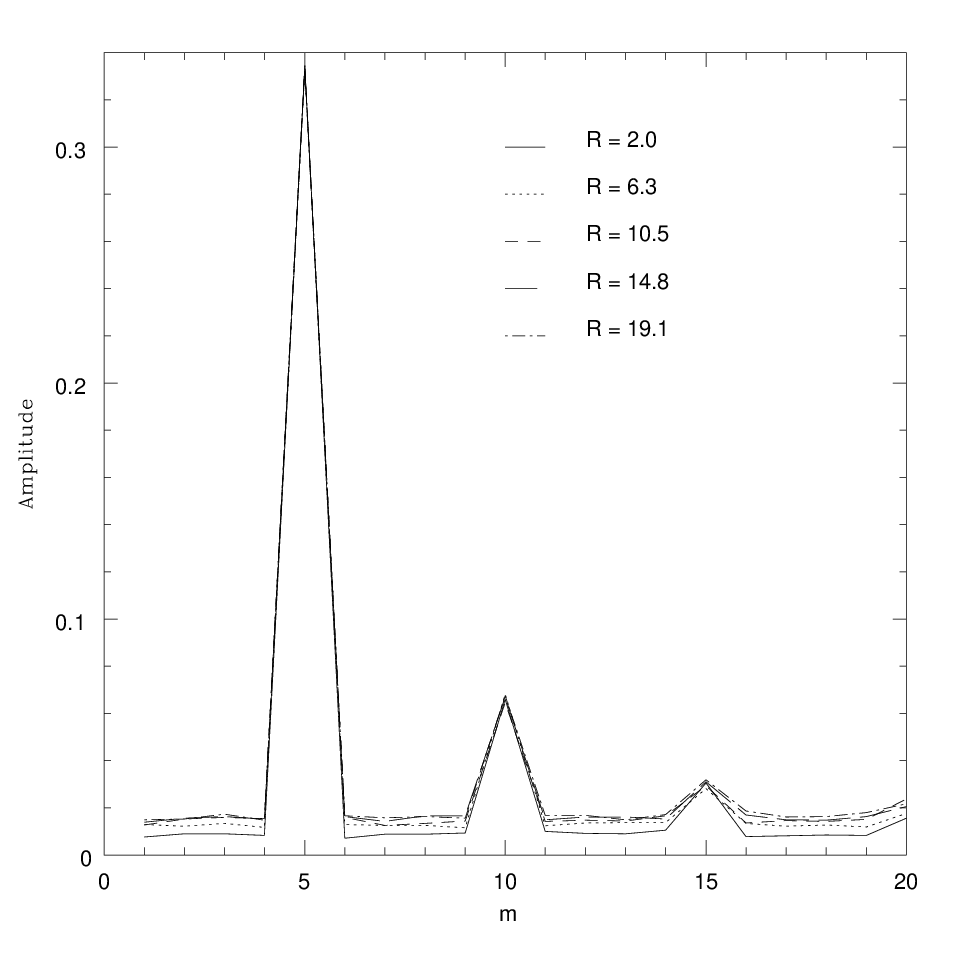
The results from the azimuthal Fourier decomposition are shown in Fig. 19, and show that the azimuthal wavenumber is resolved extremely well. The fundamental frequency is clearly dominant, with no other modes except higher harmonics present at any significant amplitude. Note that the results for the azimuthal modes show no sensitivity to the annuli used for the analysis, and are quoted for the first case in Table 3 where the annuli width correspond exactly to the radial wavelengths.
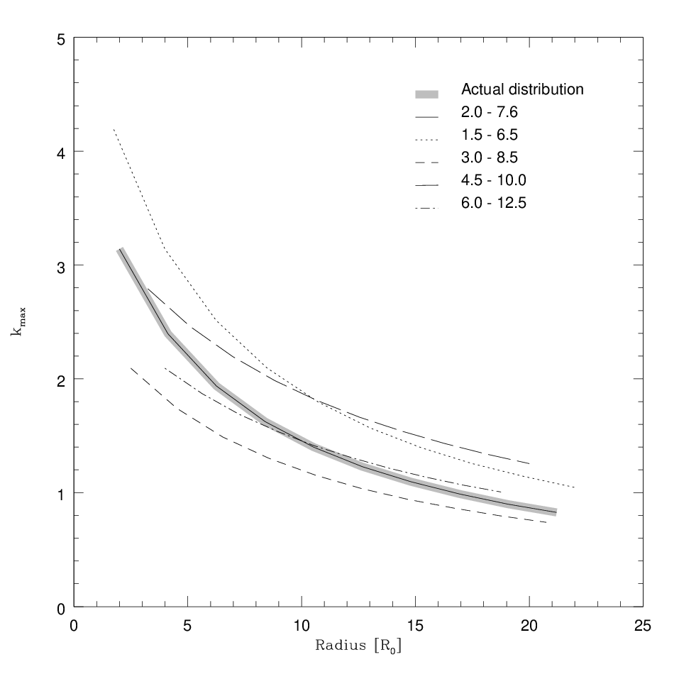
The results of the Fourier decomposition for the radial wavenumbers are shown in Fig. 20, which shows the actual distribution of wavenumbers (as calculated directly from the known distribution of wavelengths) and the distributions derived from analyses using the annuli given in Table 3. Note that the analysis using annuli that fit the wavelengths exactly correspondingly reproduces the exact result. Clearly there is scatter within the results for the radial wavenumbers, which arises from the fact that if the actual wavelength is not an integer divisor of the annulus over which the analysis is being conducted, more than one wavenumber appears to be excited. We note however that the scatter is never more than a factor of 1.5 above or below the true value, which we deem to be accurate enough for the purposes of this analysis.
Resolution Limits
Throughout this paper, we have used discs of 500,000 particles when undertaking the Fourier analysis. From the fundamental SPH resolution limit of the local smoothing length we can evaluate the maximum resolvable azimuthal and radial wavenumbers and as a function of radius throughout our discs, such that
| (A-5) |
| (A-6) |
Since the approximate expected values for radial and azimuthal wavenumbers are such that and respectively, Eqs.(A-5) and (A-6) show that the accuracy of the Fourier analysis is closely tied to the vertical resolution of the disc through . Using the average smoothing length at each radius, these resolution limits are shown in Fig. 21. We have used data from the simulation where , as this gives the most conservative limits of all our experiments.
The vertical resolution of the disc as indicated by is shown in Fig. 22 for simulations using 500,000 particles. We find that the disc thickness is covered by approximately two smoothing lengths throughout, and thus is adequately resolved. For the Fourier analysis we therefore see that the expected peak wavenumbers are resolved by a factor of approximately throughout the radial range. For the radial wavenumbers, we are primarily interested in , which is well resolved until at least , again adequate for the analyses we have undertaken. We conclude therefore that throughout the radial ranges of interest, the Fourier analyses we have presented are well resolved.

