Approximately dual frame pairs in Hilbert spaces and applications to Gabor frames
Abstract
We discuss the concepts of pseudo-dual frames and approximately dual frames, and illuminate their relationship to classical frames. Approximately dual frames are easier to construct than the classical dual frames, and might be tailored to yield almost perfect reconstruction.
For approximately dual frames constructed via perturbation theory, we provide a bound on the deviation from perfect reconstruction. An alternative bound is derived for the rich class of Gabor frames, by using the Walnut representation of the frame operator to estimate the deviation from equality in the duality conditions.
As illustration of the results, we construct explicit approximate duals of Gabor frames generated by the Gaussian; these approximate duals yield almost perfect reconstruction. Amazingly, the method applies also to certain Gabor frames that are far from being tight.
1 Introduction
Let be a separable Hilbert space with inner product . Given a frame for it is well known that there exists at least one dual frame i.e., a frame for which
Unfortunately, it is usually complicated to calculate a dual frame explicitly. Hence we seek methods for constructing approximate duals. The current paper treats the concepts of pseudo-dual and approximately dual frames and examines their properties. The idea of looking at approximately dual frames has appeared several times in the literature, for example [1, 8, 11] in the wavelet setting and [7] for Gabor systems, but our contribution is the first systematic treatment.
An approximately dual frame associated with satisfies
| (1) |
for some . (This bound is particularly interesting when is small.) We will show that any approximately dual frame generates a natural dual frame in the classical sense; further we obtain a family of frames that interpolates between the approximately dual frame and the “true” dual frame.
We also investigate the use of perturbation theory to construct approximately dual frames. There are situations where it is hard to find a dual frame for a given frame whereas a frame close to can be found for which a dual frame is known explicitly. We present conditions under which such a frame is approximately dual to , both in the case where is an arbitrary dual of and for the particular case where it is the canonical dual.
General Hilbert space estimates might of course be improved in concrete cases. For Gabor frames in we present a direct way to obtain an inequality of the type (1), based on the Walnut representation of the frame operator [15]; the obtained value measures the deviation from equality in the Gabor duality conditions.
As an illustration of the method, we construct approximately dual frames for two Gabor frames generated by the Gaussian. In these concrete cases, we obtain approximations of type (1) with very small values for .
The paper is organized as follows. Section 2 contains a few elementary definitions and results from standard frame theory. In Section 3 we introduce the new concepts of pseudo-dual and approximately dual frames, and investigate their properties. The (apparently) most useful concept of these, approximately dual frames, is studied in more detail in Section 4; in particular, we show how to obtain approximate duals via perturbation theory. The direct estimates for Gabor frames are found in Section 5, and the applications to Gabor frames generated by the Gaussian are in Section 6. Finally, an appendix collects a few examples and proofs related to classical frame theory.
2 Basic frame theory
For the introductory frame material that follows, see any standard reference on frames, such as [5], [10], [16], [2, Chapter 5].
A sequence in indexed by an arbitrary countable index set, is a frame if there exist constants such that
| (2) |
Any numbers such that (2) holds are called (lower and upper) frame bounds.
If at least the upper inequality holds, then is a Bessel sequence. For later use, note that if is a Bessel sequence then so is for any bounded operator .
Given a Bessel sequence the synthesis operator given by
is linear and bounded, with ; the series converges unconditionally for all The adjoint of is the analysis operator given by
The frame operator is . The frame operator is particularly useful if actually is a frame, but it is well defined and bounded if we just assume is a Bessel sequence.
Given a Bessel sequence , a Bessel sequence is called a dual frame if
| (3) |
Condition (3) means that analysis using followed by synthesis using yields the identity operator. We adopt the terminology of signal processing and speak then about perfect reconstruction.
One choice of dual frame is the canonical dual frame . When is redundant, infinitely many other dual frames exist.
Note that if has the upper frame bound and is a dual frame, then an application of the Cauchy–Schwarz inequality on
shows that satisfies the lower frame inequality with bound thus the sequences and are indeed frames. For later use, observe that no estimate on the upper frame bound for can be deduced from the duality condition or from knowledge about the frame bounds for , as Example A.1 in Appendix A shows.
3 Various concepts of duality
In order to apply the dual frame expansion (3) for a given frame , we need to find a dual frame . Unfortunately, it might be cumbersome — or even impossible — to calculate a dual frame explicitly. In the literature one finds only a few infinite dimensional non-tight frames for which a dual has been constructed. This paucity of constructions leads us to seek frames that are “close to dual”. We will propose two such concepts.
Suppose that and are Bessel sequences in we will denote their synthesis operators by and respectively. The operators and will be called mixed frame operators. Note that
and
Recall that and are dual frames when or .
Definition 3.1
Bessel sequences and are said to be
- •
approximately dual frames if or ,
- •
pseudo-dual frames if or is a bijection on .
In each definition, the two given conditions are equivalent, by taking adjoints. Note also that the article [4] uses the term approximate dual with a different meaning than we do here.
We illustrate the pseudo-dual idea by means of a frame characterization.
Theorem 3.2 (Characterization of frames)
Let be a Bessel sequence in . Then the following statements are equivalent.
- (a)
is a frame for .
- (b)
The frame operator is a bijection on .
- (c)
The synthesis operator is surjective onto .
- (d)
has a dual frame .
- (e)
has a pseudo-dual frame .
The new part of the theorem is the pseudo-dual statement in part (e). We need, however, some information from the proof of the known parts at several instances in our paper, so we include a full proof of Theorem 3.2 in Appendix A.
Part (b) of the theorem shows that every frame is pseudo-dual to itself. The proof of (a)(b) gives even more: in fact, denoting the frame bounds for by and , the result (16) in Appendix A shows that
| (4) |
i.e., every frame is approximately dual to the multiple of itself.
Next we establish relations among the three duality concepts.
Lemma 3.3 (Duality relations)
Let and be Bessel sequences in .
- (i)
If and are dual frames, then and are approximately dual frames.
- (ii)
If and are approximately dual frames, then and are pseudo-dual frames.
- (iii)
If and are pseudo-dual frames, then and are frames.
- (iv)
If and are pseudo-dual frames and is a bounded linear bijection, then and are pseudo-dual frames.
Proof. Statement (i) is an immediate consequence of the definitions. So is (ii), since implies is a bijection, with inverse given by a Neumann series. Statement (iii) follows from Theorem 3.2. For the proof of (iv), observe that the synthesis operator for is the assumptions of and being pseudo-dual frames and being a bijection imply that is a bijection.
The property of being a pair of pseudo-dual frames is significantly weaker than being a pair of dual frames. Nevertheless, the following proposition shows that pseudo-dual frame pairs generate dual frame pairs in a natural fashion.
Proposition 3.4 (Pseudo-duals generate duals)
If and are pseudo-dual frames, then and are dual frames.
Proof. Assuming that and are pseudo-dual frames, we know that exists and is bounded. Hence is a Bessel sequence. If we analyze with and synthesize with then we obtain the identity, since
Thus and are dual frames.
The relation of being a pair of pseudo-dual frames is symmetric: if and are pseudo-dual frames, then so are and . The pseudo-dual relation is also reflexive on the set of frames since every frame is pseudo-dual to itself, as remarked after Theorem 3.2. Transitivity of the pseudo-dual relation fails (in Hilbert spaces of dimension at least 2) by Example 4.4 below.
4 Approximately dual frames
In this section we focus on approximately dual frames and As before, we denote the associated synthesis operators by and , respectively. Our main goal is to demonstrate how one can use this concept to obtain what in engineering terms would be called “almost perfect reconstruction”.
Recall that if and are approximately dual frames then
If then we see that “almost reconstructs” , which motivates our terminology.
We first strengthen Proposition 3.4, for approximately dual frames and the associated “natural” dual frame.
Proposition 4.1
Assume that and are approximately dual frames. Then the following hold:
- (i)
The dual frame of can be written
(5) - (ii)
Given , consider the corresponding partial sum,
(6) Then is an approximate dual of . Denoting its associated synthesis operator by , we have
(7)
Proof. Assuming that and are approximately dual frames, the inverse of can be written via a Neumann series as
| (8) |
The result in (i) now follows by applying this expansion to and recalling Proposition 3.4.
For (ii), note that is a Bessel sequence since it is obtained from the Bessel sequence by a bounded transformation. And
by telescoping. Thus
Remark 4.2
In view of formula (5) in Proposition 4.1, an approximately dual frame associated with a frame can be regarded as a zero-th order approximation to the (exact) dual frame . In case is small, reconstruction using the approximate dual is close to perfect reconstruction. The result in (ii) yields a family of approximately dual frames that interpolates between the approximate dual and the dual frame ; the estimate (7) shows that by choosing sufficiently large, we can obtain a reconstruction that is arbitrarily close to perfect. The drawback of the result with respect to potential applications is the complicated structure of the operator in (6) defining the sequence .
We have now presented the basic facts for approximately dual frames. In the following, we will present concrete settings where they yield interesting new insights.
To motivate the results, we note (again) that it can be a nontrivial task to find the canonical dual frame (or any other dual) associated with a general frame We seek to connect this fact with perturbation theory by asking the following question: if we can find a frame that is close to and for which it is possible to find a dual frame , does it follow that is an approximate dual of ? We will present some sufficient conditions for an affirmative answer.
First we state a general result, valid for dual frames with sufficiently small Bessel bound; later we state a more explicit consequence for the case where is the canonical dual frame, see Theorem 4.5. Technically, we need not assume that is a frame in the general result: the frame property follows as a conclusion. On the other hand, as explained above, the main use of the result is in a setting where is known to be a frame in advance.
Theorem 4.3 (Dual of perturbed sequence)
Assume that is a sequence in and that is a frame for which
for some . Consider a dual frame of with synthesis operator , and assume has upper frame bound .
If then and are approximately dual frames, with
Proof. With our usual notation, we have since and are dual frames. Hence
It is crucial in Theorem 4.3 that the dual frame has upper frame bound less than . Otherwise need not be pseudo-dual to , let alone approximately dual, as the next example shows.
Example 4.4
Consider with the standard basis . Let and consider the frames
Write for the associated synthesis operators. Note that
this operator is neither injective nor surjective, and so and are not pseudo-dual frames. Clearly, is a frame for regardless of the choice of Now, because
the condition in Theorem 4.3 is satisfied with Thus we see that no matter how close gets to (meaning, no matter how small is), the frame is not pseudo-dual to . Note that for the frame has the upper frame bound thus, Theorem 4.3 is not contradicted.
In this example it is immediate to see that and thus and are dual frames, and so are and . In particular, the example shows that the pseudo-dual property is not transitive. The same argument applies in any separable Hilbert space of dimension at least 2.
For practical applications of Theorem 4.3, it is problematic that the Bessel bound on might increase when one reduces by taking very close to in this way, it might not be possible to get just by taking sufficiently close to . In the case when is the canonical dual of the problem does not arise: as the next result shows, if is sufficiently close to , then the canonical dual of is approximately dual to . For the statement of this result we need to assume that is a frame, since its lower frame bound controls the perturbation hypothesis.
Theorem 4.5 (Canonical dual of perturbed frame)
Let be a frame for with frame bounds Let be a sequence in for which
for some Denote the synthesis operator for by
Then is a frame. Its canonical dual frame is an approximate dual of with
where denotes the synthesis operator for .
Proof. The sequence is a frame with frame bounds and , by [2, Corollary 5.6.3]; the proof is short, and so we give it here. We have by assumption, and so
for all , from which the desired frame bounds follow easily. This part of the proof uses only .
The canonical dual frame of is with frame bounds
by [2, Lemma 5.1.6]. In terms of the synthesis operator for , the upper bound says
Theorem 4.3 therefore implies
To complete the proof, just notice this last expression is smaller than if and only if
We end this section with remarks concerning the appearance of approximate duals in the literature. Approximately dual frames have been employed in the theory of wavelets; for example, Holschneider developed a sufficient condition for a pair of wavelet systems to be approximately dual [11, Section 2.13], and Gilbert et al. [8] obtained approximate duals for highly oversampled wavelet systems by perturbing the continuous parameter system. Approximate duals have proved central to the recent solution of the Mexican hat wavelet spanning problem [1]. There the synthesizing wavelet frame is given, being generated by the Mexican hat function, and the task is to construct an approximately dual analyzing frame. Interestingly, this approximate dual construction holds in all spaces (in the frequency domain), which suggests that parts of the theory in this paper might extend usefully to Banach spaces.
Approximately dual frames in Gabor theory arose in the work of Feichtinger and Kaiblinger [7, Sections 3,4]. They studied the stability of Gabor frames with respect to perturbation of the generators and the time-frequency lattice; among many other results, they showed that a sufficiently small perturbation (measured in a specific norm) of a dual frame associated with a Gabor frame leads to an approximately dual frame. In the next sections, we construct explicit examples of approximately dual Gabor frames.
5 Gabor frames and approximate duals
The general frame estimates in Section 4 are based on operator inequalities such as the product rule . We will apply these general estimates in the next section to obtain explicit approximate duals for Gabor frames generated by a Gaussian. First, though, we will sharpen the general frame estimates in the concrete, rich setting of Gabor theory. These sharper estimates also will be applied in the next section.
A Gabor frame is a frame for of the form
for suitably chosen parameters and a fixed function called the window function. The number is called the translation parameter and is the modulation parameter. Introducing the operators
the Gabor system can be written in the short form For more information on Gabor analysis and its role in time–frequency analysis we refer to the book by Gröchenig [9].
We state now the duality conditions for a pair of Gabor systems, due to Ron and Shen [14]. We will apply the version presented by Janssen [12]:
Lemma 5.1
Two Bessel sequences and form dual frames for if and only if the equations
| (9) | |||||
| (10) |
hold a.e.
Recall that the Wiener space consists of all bounded measurable functions for which
It is well known that if then is a Bessel sequence for each choice of
Theorem 5.2
Given two functions and two parameters , let denote the synthesis operator associated with the Gabor system and the synthesis operator associated with Then
Proof. The starting point is the Walnut representation of the mixed frame operator associated with and According to Theorem 6.3.2 in [9],
Thus,
which concludes the proof.
6 Applications to Gabor frames generated by the Gaussian
The Gaussian is well known to generate a Gabor frame whenever For the case where the parameters and are equal and small, Daubechies has demonstrated that the Gabor frame generated by the Gaussian is almost tight, see [5], p.84–86 and [6], p. 980–982; in particular, the formula (4) yields almost perfect reconstruction.
Regardless of the choice of and , no convenient explicitly given expression is known for any of the dual frames associated with the Gaussian, though. We will construct explicit, approximately dual frames associated with the Gaussian, for certain choices of and . These approximately dual frames provide almost perfect reconstruction; Example 6.2 is particularly interesting because it deals with a frame that is far from being tight, i.e., no easy way of obtaining an approximately dual frame is available.
Example 6.1
Consider the (scaled) Gaussian
| (11) |
The scaling is introduced for convenience; similar constructions can be performed for other Gaussians as well. It is well known that for this Gaussian, the Gabor system forms a frame for for any sufficiently small value of the modulation parameter ; we fix in this example. Denote the synthesis operator for that frame by .
We will use the results derived in this paper to find an approximately dual Gabor frame. Let denote the eighth-order B-spline, centered at the origin. This B-spline approximates the Gaussian very well: see Figures 1 and 2. The Gabor system is a frame for , and by Corollary 3.2 in [3] it has the (non-canonical) dual frame where
| (12) |
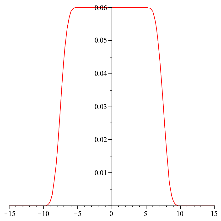
is a linear combination of translated B-splines. This is supported on and is constantly equal to on see Figure 3.
We first apply Theorem 4.3. A numerical calculation based on Theorem 9.1.5 in [2] shows that the functions form a Bessel sequence with Bessel bound
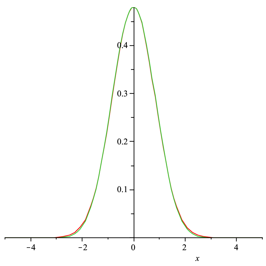
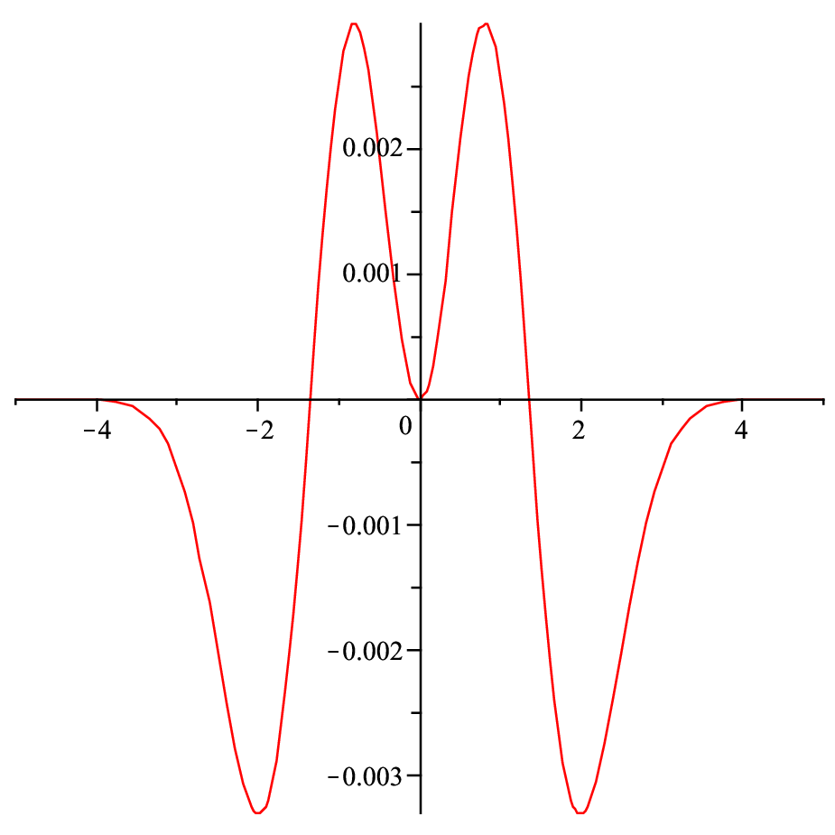
Furthermore, a second application of Theorem 9.1.5 in [2] reveals that has Bessel bound Thus the hypotheses of Theorem 4.3 are satisfied. Denoting the synthesis operator for by , we deduce that
On the other hand, an application of Theorem 5.2 immediately yields the better estimate
In terms of the Gabor systems involved, this conclusion says that
That is, analysis with the scaled Gaussian and synthesis with the function yields almost perfect reconstruction.
We note that the frame considered in this example is almost tight; thus, the approximate dual constructed here does not perform better than using a scaled version of the frame itself as approximate dual. For a frame that is far from being tight this aspect changes drastically in favor of the approximate duals considered in this paper – see Example 6.2. Lastly, we remark that other approximations to the Gaussian are possible too; instead of using B-splines and their duals from [3] we could have used certain other splines and their duals from [13].
In the next example we apply Theorem 4.5 and Theorem 5.2. Let us again consider B-spline approximation to a Gaussian. The advantage of using the canonical dual and Theorem 4.5, compared with our use of a non-canonical dual frame in Example 6.1, is that larger values of the modulation parameter can be handled. Approximating using , our approach in Example 6.1 is restricted to (the restriction comes from the underlying results in [3]); as illustration of the larger range for obtained via Theorem 4.5, we take in the next example.
Example 6.2
Let
An application of Theorem 5.1.5 in [2] shows that the functions form a frame for with frame bounds . The function
yields a close approximation of see Figure 4. A numerical calculation based on Theorem 5.1.5 in [2] shows that the functions form a Bessel sequence with Bessel bound
The function has support on an interval of length . Since the modulation parameter is smaller than and the function
is bounded above and below away from zero, it follows from Corollary 9.1.7 in [2] that the frame has the canonical dual frame where
| (13) | |||||
See Figure 5.


The frame is approximately dual to , by Theorem 4.5. Denoting their synthesis operators by and respectively, the approximation rate in Theorem 4.5 is measured by
| (14) |
On the other hand, Theorem 5.2 yields the somewhat better estimate
| (15) |
Thus the approximate dual frame almost yields perfect reconstruction.
Remark 6.3
1. In case a closer approximation than in (15) is required, an application of the iterative procedure in Proposition 4.1 (ii) can bring us as close to perfect reconstruction as desired. Letting be a Gabor frame and be an approximately dual Gabor frame , each approximate dual constructed in Proposition 4.1 will again have Gabor structure. For an easy calculation shows that will be the Gabor system where
For the particular case considered in Example 6.2, and denoting the synthesis operator for by Proposition 4.1 shows that the estimate in (14) will be replaced by
2. Another way of calculating approximate duals for Gabor frames based on would be to follow the procedure in Example 6.2 with a function of the type
for a sufficiently large interval , rather than letting be a B-spline. However, for such a function the canonical dual window associated with will not be continuous; thus, it will have bad time-frequency properties.
Acknowledgments
Laugesen thanks the Department of Mathematics at the Technical University of Denmark for travel support and a warm welcome.
Appendix A Proofs and additional examples
In this Appendix we collect some additional information related to classical frame theory.
First, we present the example announced in Section 2, showing that an estimate on the upper frame bound for a frame neither can be deduced from the fact that it is dual to a frame , nor from knowledge of the frame bounds for .
Example A.1
Consider the Hilbert space with the standard orthonormal basis . Let
Then is a frame with bounds . For any the sequence
is a dual frame of The (optimal) upper frame bound for is which can be arbitrarily large.
Exactly the same considerations apply in an arbitrary separable Hilbert space of dimension at least two.
We now state the announced proof of Theorem 3.2. The equivalences between the first four statements are well known; we include the proof in order to keep the paper self-contained, and because we refer to some of the steps elsewhere in the paper.
Proof of Theorem 3.2: First recall that and are bounded operators from to , whenever and are Bessel sequences.
(a) implies (b): First, write for the frame operator, and note it is selfadjoint. By part (a) we have for all . That is, ; following the argument by Gröchenig [9] p.91, we infer that . Thus,
| (16) | |||||
Therefore is invertible, so that is a bijection as desired.
(b) implies (c) is immediate.
(c) implies (d): consider the pseudo-inverse . Applying the Riesz representation theorem to the functional (-th component of ), we obtain some element satisfying . The sequence is Bessel, since
The analysis operator associated to the sequence equals exactly the pseudo-inverse , by construction, and so equals the identity, by the fundamental property of the pseudo-inverse. Thus is a dual frame for , and so (d) holds.
(d) implies (e) trivially.
(e) implies (a) as follows: suppose is a pseudo-dual frame for , so that is a bijection on . Then for all ,
and of course . Hence is a frame with bounds and .
References
- [1]
H.-Q. Bui and R. S. Laugesen: Frequency-scale frames and
the solution of the Mexican hat problem. Preprint, 2008.
www.math.uiuc.edu/~laugesen/ - [2] O. Christensen: Frames and bases. An introductory course. Birkhäuser, Boston, 2008.
- [3] O. Christensen and R. Y. Kim: On dual Gabor frame pairs generated by polynomials. Accepted for publication in J. Fourier Anal. Appl., 2008.
- [4] Chui, C., He, W., and Stöckler, J.: Nonstationary tight wavelet frames, I: Bounded intervals. Appl. Comp. Harm. Anal. 17 (2004), 141–197.
- [5] I. Daubechies: Ten lectures on wavelets. SIAM, Philadelphia, 1992.
- [6] I. Daubechies: The wavelet transformation, time-frequency localization and signal analysis. IEEE Trans. Inform. Theory 36 (1990), 961–1005.
- [7] H. G. Feichtinger and N. Kaiblinger. Varying the time-frequency lattice of Gabor frames. Trans. Amer. Math. Soc. 356, 2001–2023, 2004.
- [8] J. E. Gilbert, Y. S. Han, J. A. Hogan, J. D. Lakey, D. Weiland and G. Weiss. Smooth molecular decompositions of functions and singular integral operators. Mem. Amer. Math. Soc. 156, no. 742, 74 pp., 2002.
- [9] K. Gröchenig: Foundations of time-frequency analysis. Birkhäuser, Boston, 2000.
- [10] C. Heil and D. Walnut: Continuous and discrete wavelet transforms. SIAM Review 31, 628–666, 1989.
- [11] M. Holschneider: Wavelets. An analysis tool. Oxford Mathematical Monographs. Oxford Science Publications. The Clarendon Press, Oxford University Press, New York, 1995.
- [12] A. J. E. M. Janssen: The duality condition for Weyl-Heisenberg frames. In “Gabor analysis: theory and applications” (eds. H.G. Feichtinger and T. Strohmer). Birkhäuser, Boston, 1998.
- [13]
R. S. Laugesen: Gabor dual spline windows.
Preprint, 2008.
www.math.uiuc.edu/~laugesen/ - [14] A. Ron and Z. Shen: Frames and stable bases for shift-invariant subspaces of . Canad. J. Math. 47, 1051–1094, 1995.
- [15] D. Walnut: Continuity properties of the Gabor frame operator. J. Math. Anal.Appl. 165, 479–504, 1992.
- [16] R. Young: An introduction to nonharmonic Fourier series. Academic Press, New York, 1980 (revised first edition 2001).
Ole Christensen, Department of
Mathematics, Technical University of
Denmark,
Building 303, 2800 Lyngby, Denmark Ole.Christensen@mat.dtu.dk
Richard S. Laugesen, Department of Mathematics, University of Illinois at Urbana–Champaign, Urbana, IL 61801, U.S.A. Laugesen@illinois.edu