Nuclear State Preparation via Landau-Zener-Stückelberg transitions in Double Quantum Dots

Introduction— Since the electron spin in quantum dots (QDs) has been proposed as a qubit [1], much progress has been made to develop reliable semiconductor devices, mostly with GaAs, in which only a single electron can be confined and its spin can be controlled [2]. Despite the achievement of reliable control, spin decoherence due to the hyperfine interaction with the surrounding nuclear spins remains a major problem [3]. In double QDs, where the singlet ($\mathrm{S}$) and one of the triplet ($\mathrm{T}_{0}$) states can be chosen as an effective two-level system to implement a qubit [4, 5, 6], it has been shown that the probability, averaged over many runs of the experiment, to find the system in the singlet state at time $t>0$, having prepared a singlet at time $t=0$, is a decaying oscillating function $\propto\cos(Jt)\exp(-(t/T_{2}^{*})^{2})$ [8, 7], with singlet-triplet exchange splitting $J$ and decoherence time $T_{2}^{*}$.

An important goal in the quest to overcome decoherence of spin qubits in solid-state devices is to find mechanisms that allow for an increase in $T_{2}^{*}$. Spin echo has been used to reveal $T_{2}\approx\mathrm{\mu s}\gg T^{*}_{2}$ [8] which sets the scale that can be achieved by nuclear-state preparation. In principle, it is possible to reduce the nuclear fluctuations, thus prolonging $T_{2}^{*}$, by projecting the nuclear state into (approximate) Overhauser eigenstates with either electrical or optical means [9, 10] or by polarizing the nuclear spins [11, 12]. However, a sizable enhancement of electron spin coherence would only be realized for a polarization of more than 99% [13], which so far has not been achieved.

Reilly et al. [14] have experimentally studied adiabatic transitions of two electrons in a pair of tunnel-coupled QDs from a spin singlet $\mathrm{S}(2,0)$, with both electrons in the same QD and total spin $0$, across an energy level anti-crossing to a spin triplet $\mathrm{T}_{+}(1,1)$, with one electron in each QD and total spin $1$ (see Fig. 1). Due to angular momentum conservation, the hyperfine-induced transition $\mathrm{S}$-$\mathrm{T}_{+}$ involves an electron spin flip accompanied by a nuclear spin flop. In the experiment, the process was repeated many times with intermediate fast resetting to the singlet state ($200\,\mathrm{ns}$). If the slow $\mathrm{S}$-$\mathrm{T}_{+}$ transition was fully adiabatic and the nuclear spin polarization sufficiently long-lived, this cycle should allow for complete nuclear polarization as the number of cycles becomes comparable to the number of nuclear spins in the QDs (typically about $10^{5}$ to $10^{6}$). However, a polarization of only about 1% was achieved. Nevertheless, the coherence time measured in the $\mathrm{S}$-$\mathrm{T}_{0}$ subspace was improved by a factor of up to 70 [14] which can be attributed to the preparation of a suitable nuclear state. A previous theoretical model has been used to calculate the evolution of up to $36$ nuclear spins per dot for an initial mixed state with fixed angular momentum per dot [15].

Here, we propose a theoretical model of nuclear state preparation taking into account all possible angular momenta, up to $200$ nuclear spins per QD, and the possibility of partially adiabatic transitions. Such transitions can explain the smallness of the nuclear polarization generated while allowing for a weak measurement [16] of the nuclear state. The repeated weak measurements at each cycle lead to nuclear state narrowing and, as a consequence, to a prolongation of the spin singlet-triplet coherence. The main feature of our theoretical model is the description of the partially adiabatic $\mathrm{S}$-$\mathrm{T}_{+}$ transition by the Landau-Zener-Stückelberg (LZS) theory [17, 18, 19]. Due to the high degeneracy of the nuclear spin state and the finite sweep time, we use suitable generalizations of the LZS model [20, 21].

Model— We derive the Hamiltonian describing the partially adiabatic dynamics at the $\mathrm{S}$-$\mathrm{T}_{+}$ anti-crossing. We start with the spin-preserving part $H_{0}$ of the Hamiltonian, with $[H_{0},S_{z}]=0$, describing the coupling between two electrons in a double QD in a magnetic field $B$,

where $g^{*}$ denotes the effective Landé g-factor ($-0.44$ for GaAs), $\mu_{\mathrm{B}}$ the Bohr magneton, and the indices $i=1,2$ and $\sigma=\uparrow,\downarrow$ label the dot number and spin. The first term is the single-particle energy of the confined electrons, the second accounts for the Coulomb energy $u$ of two electrons on the same QD, and the last for the electron tunneling with strength $\tau$ between the dots.

The diagonalization of the first two terms of Eq. (1) leads to the relevant states of a double QD: the singlets $\mathrm{S}(0,2)$, $\mathrm{S}(2,0)$, $\mathrm{S}(1,1)$ and triplets $\mathrm{T}_{\pm,0}(1,1)$, where $(l,r)$ indicates the number of electrons in the (left, right) dot. The other states can be neglected as they have energies much higher than those considered here. The degeneracy of the singlets $\mathrm{S}(2,0)$ and $\mathrm{S}(1,1)$ at $\varepsilon=\pm u$ is lifted by the inter-dot tunneling, resulting in a splitting of $\sqrt{2}\tau$. The energy levels as a function of the bias $\varepsilon=\varepsilon_{1}-\varepsilon_{2}$ are shown in Fig. 1(a). At the degeneracy $\varepsilon=\varepsilon^{*}$ of the singlet $\mathrm{S}(1,1)$ and the triplet $\mathrm{T}_{+}(1,1)$, the hyperfine interaction between the electron spins $\mathbf{S}_{i}$ and the nuclear spins $\mathbf{I}_{i}^{k}$ opens a splitting $\Delta_{\mathrm{HF}}$. The contact hyperfine Hamiltonian is given by $H_{\mathrm{HF}}=\mathbf{S}_{1}\cdot\mathbf{h}_{2}+\mathbf{S}_{2}\cdot\mathbf{h}_{2}$ where $\mathbf{h}_{\mathrm{i}}=\sum_{k=1}^{n(i)}A_{i}^{k}\mathbf{I}_{i}^{k}$ is the Overhauser (effective nuclear field) operator. The sum runs over the $n$ nuclear spins in dot $i$, $A_{i}^{k}=v_{k}\nu_{0}\left|\Psi(\mathbf{r}_{k})\right|^{2}$ is the hyperfine coupling constant with the $k$-th nucleus in dot $i$, with $\Psi(\mathbf{r}_{k})$ the electron wave function, $\nu_{0}$ the volume of the unit cell and $v_{k}$ the hyperfine coupling strength. Introducing $S_{i}^{\pm}=S_{i}^{x}\pm iS_{i}^{y}$ and $h_{i}^{\pm}=h_{i}^{x}\pm ih_{i}^{y}$, we write $H_{\mathrm{HF}}$ as

Since $\tau\gg\Delta_{\mathrm{HF}}$, we can use $H=H_{0}+H_{\mathrm{HF}}$ to derive an effective Hamiltonian for the subspace spanned by $\{|\mathrm{S},j_{1},m_{1},j_{2},m_{2}\rangle\}$ and $\{|\mathrm{T}_{+},j_{1},m_{1}^{\prime},j_{2},m_{2}^{\prime}\rangle\}$, where $j_{i}$ is the total nuclear angular momentum in dot $i$ and $m_{i}$ its projection along $B$,

where $q=\mathrm{S},\mathrm{T}$, $|\mathbf{\chi}\rangle=|j_{1},m_{1},j_{2},m_{2}\rangle$, and $E_{\mathrm{S},\mathbf{\chi}}(\varepsilon)=E_{\mathrm{S}}(\varepsilon)$, and $E_{\mathrm{T},\mathbf{\chi}}(\varepsilon)=E_{\mathrm{T}}(\varepsilon)+\langle h^{z}_{1}+h^{z}_{2}\rangle_{\mathbf{\chi}}/2+g^{*}\mu_{\mathrm{B}}B$.

Method— With a time-dependent bias $\varepsilon=\varepsilon(t)$, the Hamiltonian (3) is of the form $H=H_{0}(t)+H_{\mathrm{int}}$, as the one studied by LZS to derive the staying and transition probabilities $P_{\mathrm{a}}$ and $P_{\mathrm{na}}$ between two levels $|1\rangle$ and $|2\rangle$ driven through resonance between $t_{\mathrm{i}}=-\infty$ and $t_{\mathrm{f}}=+\infty$ by assuming that their energy difference is a linear function of time, $\Delta(t)=\left|E_{\mathrm{S},\mathbf{\chi}}(t)-E_{\mathrm{T},\mathbf{\chi}}(t)\right|=\alpha t$ with the well-known result $P_{\mathrm{a}}=1-P_{\mathrm{na}}=1-\exp(-2\pi|\langle 1|H_{\mathrm{HF}}|2\rangle|^{2}/\alpha\hbar)$. Here, we study the effect that the transitions can have on the nuclear difference field $\delta h^{z}=h_{1}^{z}-h_{2}^{z}$ and more precisely on its fluctuations $\sigma^{(z)}=\sqrt{\left\langle(\delta h^{z})^{2}\right\rangle-\left\langle\delta h^{z}\right\rangle^{2}}$ that are responsible for the qubit decoherence via $T_{2}^{*}=\hbar/\sigma^{(z)}$ [2, 23].

To study the evolution of $\sigma^{(z)}$, we compute the new state of the system after each cycle, which consists of a forward and a return sweep. The state of the system after the forward sweep results from the time evolution operator generated by (3); the resulting state is taken as the initial condition for the return sweep which is performed sufficiently fast to ensure a sudden parameter change without change in the state. As in the original LZS model, we assume a linear dependence $\Delta(t)=\alpha t$ throughout. Moreover, to make the problem treatable, we assume a constant hyperfine coupling $A_{k}\rightarrow\bar{A}$ and the nuclear spins to be $1/2$ (in reality the nuclear species of GaAs have spin $3/2$). Before treating the case of many nuclear spins, we explain the main ideas by considering the simple case of one nuclear spin in dot $1$ and none in dot $2$. The initial nuclear state is assumed to be an incoherent mixture of spin up and down; its density matrix $\rho^{(0)}_{\mathrm{n}}$ has matrix elements $\rho^{(0)}_{ij}=\delta_{ij}/2$ with $i,j=\uparrow,\downarrow$. The initial mean value and standard deviation for $\delta h^{z}$ are $\langle\delta h^{z}\rangle_{0}=0$ and $\sigma_{0}^{(z)}=\bar{A}/2$. We now assume that after a cycle, a measurement of the electron spin (via charge) is performed to determine if a flip-flop has occurred. If a singlet is detected, the nuclear density matrix becomes $\rho^{(1),\mathrm{S}}_{\uparrow\uparrow}=e^{-\eta}/2P_{\mathrm{S}}$, $\rho^{(1),\mathrm{S}}_{\downarrow\downarrow}=1/2P_{\mathrm{S}}$, and $\rho^{(1),\mathrm{S}}_{\uparrow\downarrow}=\rho^{(1),\mathrm{S}}_{\downarrow\uparrow}=0$, with $\eta=\pi\bar{A}^{2}/\alpha\hbar$ and the probability to measure a singlet, $P_{\mathrm{S}}=(e^{-\eta}+1)/2$. In this new state, $\langle\delta h^{z}\rangle_{1}=\bar{A}(e^{-\eta}-1)/2(e^{-\eta}+1)$ and $\sigma_{1}^{(z)}=(\bar{A}/2)\cosh^{-1}(\eta/2)$. In the “fast” limit $\alpha\to\infty$, we find $\rho^{(1),\mathrm{S}}_{\mathrm{n}}=\rho^{(0)}_{\mathrm{n}}$ therefore the variance is unchanged, $\sigma_{1}^{(z)}=\sigma_{0}^{(z)}$. In the “slow” limit $\alpha\to 0$, we have $\rho^{(1),\mathrm{S}}_{\downarrow\downarrow}=1$ while all other elements of $\rho^{(1),\mathrm{S}}_{\mathrm{n}}$ vanish, such that $\sigma_{1}^{(z)}=0$, describing a strong (projective) measurement of the nuclear spin. For $0<\alpha<\infty$, the detection of a singlet induces a weak measurement which decreases the fluctuations, $\sigma_{1}^{(z)}<\sigma_{0}^{(z)}$. On the other hand, if a triplet is measured, we have $\rho^{(1),\mathrm{T}}_{\uparrow\uparrow}=\rho^{(1),\mathrm{T}}_{\uparrow\downarrow}=\rho^{(1),\mathrm{T}}_{\downarrow\uparrow}=0$ and $\rho^{(1),\mathrm{T}}_{\downarrow\downarrow}=1$ independently of $\alpha$; in this case the nuclear spin is projected on the down state. We conclude that it is possible to reduce the fluctuations of the nuclear spins without fully polarizing them. Below, we show that the same mechanism works also for a system with many nuclear spins.

For $n\gg 1$, the nuclear states are highly degenerate and the LZS propagator from the simple case cannot be used anymore. An elegant solution to derive the LZS propagator for degenerate systems consists in applying the unitary Morris-Shore (MS) transformation to the LZS Hamiltonian to reduce the dynamics into sets of decoupled single states and independent two-level systems [20]. Because $H_{\mathrm{HF}}$ exclusively couples states of the form $|\mathrm{S},j_{1},m_{1},j_{2},m_{2}\rangle\equiv|0\rangle$ to the degenerate states $|\mathrm{T_{+}},j_{1},m_{1}-1,j_{2},m_{2}\rangle\equiv|1\rangle$ and $|\mathrm{T_{+}},j_{1},m_{1},j_{2},m_{2}-1\rangle\equiv|2\rangle$, the LZS Hamiltonian can be brought into a block diagonal form. The MS basis is found by diagonalizing

where $V_{ij}=\langle i|H_{\rm int}|j\rangle$, $a_{i}=\sqrt{j_{i}(j_{i}+1)-m_{i}(m_{i}-1)}$. The eigenstates are $|0\rangle$ and $|1^{\prime}\rangle=\left(a_{1}|1\rangle+a_{2}|2\rangle\right)/a_{0}$ associated with the eigenvalue $\lambda^{2}=\bar{A}^{2}/8a_{0}^{2}$, and $|2^{\prime}\rangle=\left(a_{1}|1\rangle-a_{2}|2\rangle\right)/a_{0}$ with eigenvalue $0$, where $a_{0}^{2}=a_{1}^{2}+a_{2}^{2}$. The states with the same eigenvalues are coupled with strength $\lambda$. The state $|2^{\prime}\rangle$ is a “dark state”, as it does not couple to other states. In the subspace spanned by $|0\rangle$ and $|1^{\prime}\rangle$, the time-dependent Schrödinger equation with the initial state $|0\rangle$ at time $t_{\mathrm{i}}$ can be solved and thus the LZS propagator elements $U_{0\,i^{\prime}}^{\mathrm{MS}}$ can be calculated [21]. In order to express the solution in the original basis, we perform the inverse MS transformation to find the matrix elements $U_{0\,i}=(a_{i}/a_{0})U_{0\,i^{\prime}}^{\mathrm{MS}}$. We also account for finite time propagation and thus avoid the unphysical situations of infinite energy that arises for couplings that do not vanish when $t\rightarrow\pm\infty$, and infinite detuning as we assume $\Delta(t)=\alpha t$. The finite-time solution also allows us to model the situation in the experiment [14] where mixing between $\mathrm{T}_{0}(1,\,1)$ and the $\mathrm{S}(1,\,1)$ states must be avoided.

At typical operating temperatures and fields, where $k_{B}T\gg g_{\mathrm{N}}\mu_{\mathrm{N}}B$, the initial nuclear density matrix can be assumed to be diagonal, $\rho_{\mathrm{n}}^{(0)}=\sum_{\mathbf{\chi}}p(\mathbf{\chi})|\mathbf{\chi}\rangle\langle\mathbf{\chi}|$ with a uniform distribution of states $\chi$. At $120\,\mathrm{mK}$ and $100\,{\rm mT}$, we have $k_{\mathrm{B}}T\sim 10^{-5}\,\mathrm{eV}$ and $g_{\mathrm{N}}\mu_{\mathrm{N}}B\sim 10^{-9}\,\mathrm{eV}$. The joint probability $p(\mathbf{\chi})$ can be factorized into $p^{\prime}(j_{1},m_{1})p^{\prime}(j_{2},m_{2})$ since the dots are initially independent, with $p^{\prime}(j_{i},m_{i})=g(j_{i})f(m_{i}|j_{i})$, where $g(j_{i})$ is the probability for total nuclear angular momentum $j_{i}$ and $f(m_{i}|j_{i})=[\theta(j_{i}+m_{i})-\theta(j_{i}-m_{i})]/(2j_{i}+1)$ is the equally distributed conditional probability of having a magnetization $m_{i}$ given $j_{i}$, and $\theta$ is the Heaviside function with $\theta(0)=1$. The probability distribution $g(j_{i})=G(j_{i})/\sum_{j_{i}}G(j_{i})$ is found by counting how many times $G(j_{i})$ an irreducible representation of dimension $2j_{i}+1$ occurs.

After the forward sweep of the $k$-th cycle, the state is $\rho^{(k+1)}=U\rho^{(k)}U^{{\dagger}}$, with $\rho^{(0)}=|\mathrm{S}\rangle\langle\mathrm{S}|\otimes\rho^{(0)}_{\mathrm{n}}$. The back sweep will act as a measurement of the final configuration of the electronic system. After the LZS transition the charge configuration of the system is $(1,1)$ independent of the spin, but after the back sweep it is a superposition of $\mathrm{T}_{+}(1,1)$ and $\mathrm{S}(2,0)$ which has a relatively fast decay time $\tau\sim 1\,\mathrm{ns}$ [22], such that the electronic system will evolve with probability $P_{\mathrm{S}}$ to the singlet $\mathrm{S}(2,0)$ and with probability $P_{\mathrm{T}}$ to the triplet $\mathrm{T}_{+}(1,1)$ after a time $\tau$. This provides a way to determine if the system has evolved adiabatically or not during the forward sweep. We write $\rho^{(k+1)}=P_{\mathrm{S}}\rho_{\mathrm{S}}^{(k+1)}+P_{\mathrm{T}}\rho_{\mathrm{T}}^{(k+1)}$ to describe the mixture of the ensembles that have evolved adiabatically and non-adiabatically in the forward sweep. After a time $\tau$, this state will collapse either to $\rho_{\mathrm{S}}^{(k+1)}$ or $\rho_{\mathrm{T}}^{(k+1)}$ with probability $P_{\mathrm{S}}$ and $P_{\mathrm{T}}$, respectively, with ($q=\mathrm{S},\mathrm{T}$),

where $M_{q}=|q\rangle\langle q|$ is the projection operator describing a strong measurement in the charge sector. If a singlet ($q=\mathrm{S}$) or triplet ($q=\mathrm{T}$) is detected after the $(k+1)$-th sweep, we update $\rho_{\mathrm{n}}$ according to

In the case of a triplet ($q=\mathrm{T}$), we must also take into account the nuclear spin flop,

After a flip-flop process, the crossing point $\varepsilon^{*}$ moves slightly because of the change in the total magnetic field $\mathbf{B}+(\mathbf{h}_{1}+\mathbf{h}_{2})/g^{*}\mu_{\mathrm{B}}$ and affects the initial and final times of the LZS transitions. With the convention that $t=0$ at the initial anti-crossing point, the time shift is $t_{\mathrm{i}}\rightarrow t_{\mathrm{i}}+\delta t$, $t_{\mathrm{f}}\rightarrow t_{\mathrm{f}}+\delta t$, with $\delta t=\bar{A}/\alpha$.

We have performed a Monte Carlo simulation where $t_{\mathrm{i}}=-30\,\mathrm{ns}$ and $t_{\mathrm{f}}=20\,\mathrm{ns}$, such that the duration of the first sweep is the same as in [14]. Our choice for $\alpha$ satisfies the conditions $\lambda\ll\alpha t_{\mathrm{i}}$ and $\lambda\ll\alpha t_{\mathrm{f}}\ll g^{*}\mu_{\mathrm{B}}B$ that hold for a system far from resonance at the beginning and at the end of the first cycles, and with a final difference in energy smaller than the Zeeman splitting. The order of magnitude of $\lambda$ is determined by looking at the case of the most likely $j_{i}$, which is $\sim\sqrt{n}$, with $m_{i}=0$ to consider the strongest coupling in that subspace. The number of spins is currently limited to $n=200$ per dot by the computational power at our disposal. This limitation has a side effect on the choice of the hyperfine coupling constant. For large spin systems, one has $\bar{A}=\frac{A}{n}$ with $A=90\,\mathrm{\mu eV}$ for GaAs, but for dilute systems $\bar{A}$ can be crucially smaller, therefore we choose $\bar{A}=9\,\mathrm{neV}$ [24]. Thus, $\lambda\sim 10^{-8}\,\mathrm{eV}$ so that $\alpha t_{\mathrm{f}}$ must be of the order of $10^{-7}\,\mathrm{eV}$ since $\left|g^{*}\mu_{\mathrm{B}}B\right|\simeq 2.3\,\mathrm{\mu eV}$. This implies that $\alpha$ must be between $10$ and $50\,\mathrm{eV\,s^{-1}}$, which also satisfies the condition on $\alpha t_{\mathrm{i}}$.

Results— In Fig. 2(a), we plot the evolution of $\sigma^{(z)}$, averaged over $160$ runs, as a function of the number of cycles for $\alpha=11\,\mathrm{eV\,s^{-1}}$. Since the reduction of $\sigma^{(z)}$ persists in the average, a read-out of the charge state after each cycle is not required.

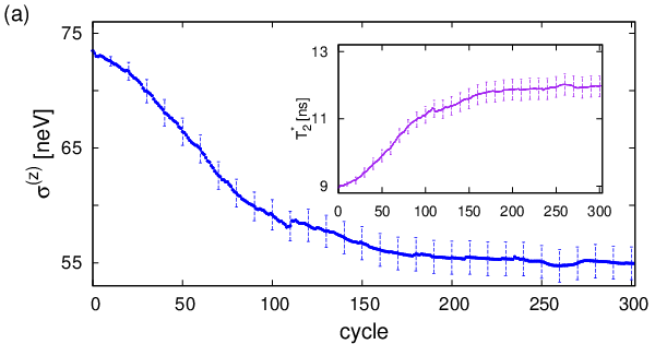
When the polarization reaches about $8\%$ (generally at $\approx 1/\sqrt{n/2}$) the nuclear spins approach a “dark state” preventing further polarization. We plot in Fig. 2(b) the average probability $P_{\mathrm{S}}$ of measuring a singlet as a function of the number of cycles. $P_{\mathrm{S}}$ can be measured in the $\mathrm{S}$ - $\mathrm{T}_{+}$, as it was done for $\mathrm{S}$ - $\mathrm{T}_{0}$ [8].

Conclusion— We have developed a model to explain the increase of $T^{*}_{2}$ in double QDs via the tuning of two electrons across an energy level anti-crossing between $\mathrm{S}(2,0)$ and $\mathrm{T}_{+}(1,1)$. Our model is based on the possibility of partially adiabatic transitions which are described by a generalized LZS theory. We have shown that the cycling combined with a spin-to-charge conversion to the $(1,1)$, respectively $(2,0)$, configuration induces a weak measurement on the nuclear state which strongly contributes in the suppression of the nuclear fluctuations. An experimental confirmation of the predicted weak measurement would be provided by measuring $P_{\mathrm{S}}\approx 1$ and at the same time an increase in $T_{2}^{*}$ as a function of the number of cycles.

Using a Monte-Carlo algorithm for $n=200$ nuclear spins per QD, we find an enhancement of the electron spin coherence time $T_{2}^{*}=\hbar/\sigma^{(z)}$ by a factor of $\sim 1.34$ after 300 cycles. While the initial $\sigma_{\mathrm{i}}^{(z)}\propto\sqrt{n}$, the final $\sigma_{\mathrm{f}}^{(z)}$ is mainly determined by the preparation mechanism and is approximatively independent of $n$. Therefore, we expect $T_{2,\mathrm{f}}^{*}/T_{2,\mathrm{i}}^{*}=\sigma_{\mathrm{i}}^{(z)}/\sigma_{\mathrm{f}}^{(z)}\propto\sqrt{n}$, and we estimate $T_{2,\mathrm{f}}^{*}/T_{2,\mathrm{i}}^{*}\approx 94$ for $n\approx 10^{6}$. This scaling stops when $T_{2}^{*}\approx T_{2}$ or before if dipolar interaction effects are taken into account. Future calculations for more spins will allow more direct comparison with experiments. Our results also apply for QDs with fewer nuclear spins e.g. in Si, ZnO, carbon nanotubes, or graphene.

Acknowledgments— We thank M. Braun and A. Romito for useful discussions. We acknowledge funding from the DFG within SPP 1285 “Spintronics” and FOR 912, and from the Swiss SNF via grant no. PP002-106310.

References

- [1] D. Loss, D. P. DiVincenzo, Phys. Rev. A 57, 120 (1998).
- [2] R. Hanson et al., Rev. Mod. Phys 79, 1217 (2007).
- [3] A. V. Khaetskii, D. Loss, L. Glazman, Phys. Rev. Lett. 88, 186802 (2002).
- [4] J. Levy, Phys. Rev. Lett. 89, 147902 (2002).
- [5] J. M. Taylor et al., Nature Physics 1, 177 (2005).
- [6] R. Hanson, G. Burkard, Phys. Rev. Lett. 98, 050502 (2007).
- [7] W. A. Coish, D. Loss, Phys. Rev. B 72, 125337 (2005).
- [8] J. R. Petta et al., Science 309, 2180 (2005).
- [9] D. Klauser, W. A. Coish, D. Loss, Phys. Rev. B 73, 205302 (2006).
- [10] D. Stepanenko, G. Burkard, G. Giedke, A. Imamoglu, Phys. Rev. Lett. 96 136401, (2006).
- [11] G. Burkard, D. Loss, D. P. DiVincenzo, Phys. Rev. B 59, 2070 (1999).
- [12] J. R. Petta et al., Phys. Rev. Lett. 100, 067601 (2008).
- [13] W. A. Coish, D. Loss, Phys. Rev. B 70, 195340 (2004).
- [14] D. J. Reilly et al., Science 321, 817 (2008).
- [15] G. Ramon, X. Hu, Phys. Rev. B 75, 161301 (2007).
- [16] Y. Aharonov, L. Vaidman, quant-ph/0105101v2 (2007).
- [17] L. D. Landau, Phys. Z. Sowjetunion 2, 46 (1932).
- [18] C. Zener, Proc. R. Soc. A 137, 696 (1932).
- [19] E. C. G. Stückelberg, Helv. Phys. Acta 5, 369 (1932).
- [20] G. S. Vasilev, S. S. Ivanov, N. V. Vitanov, Phys. Rev. A 75, 013417 (2007).
- [21] N. V. Vitanov, B. M. Garraway, Phys. Rev. A 53, 4288 (1996).
- [22] T. Hayashi et al., Phys. Rev. Lett. 91, 226804 (2003).
- [23] Writing , with and (), one finds that only the difference operators lead to the decoherence () of the qubit.
- [24] The choice of is made such that the most likely is the same for and .