Classical ${\cal{N}}=8$ supergravity (SG) has, in addition to 8 local supersymmetries, a local $SU(8)$ symmetry and a hidden global $E_{7(7)}$ symmetry [1],[2] on shell, when the exact non-linear equations of motion are satisfied. The $E_{7(7)}$ symmetry is realized linearly and independently from the local $SU(8)$ symmetry and it acts on 133 scalars present in the classical action before gauge-fixing, as well as on the vectors of the theory. The gauge-fixing can use the 63 local parameters of $SU(8)$ to remove 63 non-physical scalars so that only 70 physical scalars are left. This leads to a non-linear realization of the $E_{7(7)}$ on the remaining 70 massless scalar fields. The $E_{7(7)}$ transformation has to be performed simultaneously with the gauge preserving field dependent $SU(8)$ transformation which was specified in [3]. In the light-cone gauge the first terms in the coupling constant expansion of $E_{7(7)}$  symmetry were recently presented in [4].

The purpose of this note is to study consequences of the non-linearly realized $E_{7(7)}$ symmetry for the one-soft-scalar emission. In our study of the low-energy theorems [5, 6] in application to ${\cal{N}}=8$ SG we will use the approach developed in [7, 8] where the conserved current of the non-linearly realized ${G/H}$ symmetry plays the major role. The corresponding Noether current was presented in [3] following the procedure developed for the general case of duality symmetries in [9].

Recently Bianchi, Elvang and Freedman [10] were looking for the footprint of $E_{7(7)}$ in tree diagrams of ${\cal{N}}=8$ SG.¹¹ 1 The main results of the paper [10] is in a construction of the generating functions for the $\cal N$=8 SG amplitudes and their relation to $\cal N$=4 Yang Mills amplitudes. The expectation was to reveal the low energy theorems associated with the non-linear realization of symmetries like in pion physics [5, 6]. They have computed in [10] the one-soft-boson limit of tree diagrams using the Feynman rules and found that it always vanishes. Since there are cubic interactions in the theory, the vanishing soft-boson limit of all tree amplitudes was not an obvious feature of the theory but came out as the result of careful computations. A different setting for the study of the low-energy theorem was suggested in [11] by Arkani-Hamed, Cachazo and Kaplan. They used a specific supersymmetric deformation of the $\cal N$=8   SG to complex momenta which provides a set of recursion relations reducing all amplitudes to three point amplitudes. This takes place due to a remarkable behavior of $\cal N$=8   SG at large complex momenta. They studied the 3-point amplitudes which do not vanish on shell for the complex momenta. They established that in the one-soft boson limit these 3-point amplitudes vanish. This means, via the recursion relations, that the one-soft boson limit for all on shell tree amplitudes vanishes. They also studied a double soft limit of the amplitudes when two scalars are soft and found that it is related to an $SU(8)$ rotation of the amplitude without soft scalars.

In both of these references, [10] and [11], the soft limit of the amplitudes are directly computed and shown to vanish. Those amplitudes are related to the low-energy theorem for an $E_{7(7)}$  symmetry, but, by themselves, neither prove nor disprove the $E_{7(7)}$  symmetry.

In our approach here we will start with the $E_{7(7)}$  symmetry and consider the consequences of the Noether current conservation. The current $J_{\mu}$ consists of the linear part, proportional to the derivative of a scalar $J_{\mu}^{\rm lin}$, and a non-linear part $J_{\mu}^{\rm nonlin}$, which starts as a quadratic function of various fields. The total current conservation relates the linear part to the non-linear part

One can therefore derive the relation between the amplitudes

The left hand side of eq. (1.2) is related to the amplitude with the scalar emission ${\cal M}(\alpha\rightarrow\beta+\pi(k))$ since $\partial^{\mu}J_{\mu}^{\rm\,lin}\sim\Box_{x}\pi(x)$. When the scalar momentum $k$ is soft, the right hand side of the equation is proportional to amplitude without a scalar, where only the diagrams with singularities in the soft limit should be taken into account. The actual computation in general [7] is reduced to the computation of the divergence of the non-linear part of the Noether current between various one-particle states $\langle i|$ and $|j\rangle$ divided by such singular propagator:

This expression was introduced in [8] and we will refer to it as ‘axial’ charge, since it coincides with the usual axial charge $g_{A}\,(\sim 1.257)$ for the nucleon case in the pion physics. Clearly, there is one level of softness $k$ in the numerator due to the factor $\partial$, but there is a singularity from the propagator in the diagram, which may cancel this $k$, and the soft limit of the ${\cal M}(\alpha\rightarrow\beta+\pi(k))$ may be non-trivial. However, if $\langle i|\partial^{\mu}J_{\mu}^{\rm\,nonlin}|j\rangle$ is as soft as two powers in $k$, the amplitude ${\cal M}(\alpha\rightarrow\beta+\pi(k))$ will vanish in the soft limit.

The discussion above is general and not restricted to any particular level of perturbation theory. This is provided that the linear part $J_{\mu}^{\rm\,lin}$ is understood to be the part of the current operator which gives the linear term not in the scalar field but in the scalar asymptotic field, that is, the whole part yielding the single massless scalar pole terms (the category A diagram in Fig. 1 below). The full expression of the Noether current is known [3]. Its matrix element between the external one-particle states has to be computed in the soft-scalar limit to establish the low-energy theorem. In this paper, however, we will limit ourselves with the computation of the ‘axial’ charge only at the tree level.

First we will provide in Sec. 2 a calculational tool to derive the low-energy theorem for theories with non-linear realization of a symmetry with scalars in ${G}/{H}$ coset space. The low-energy theorem in eq. (2.16) relates an arbitrary amplitude with an extra soft scalar to the amplitude without such a scalar [7]. The relation between these amplitudes is defined by the ‘axial’ charge [8], which may or may not vanish, in general. In Sec. 3 we explain the subtleties with the Noether current in $\cal N$=8   SG, which are due to explicit appearance of the dual vector fields in the current. These dual fields are not present in the Lagrangian. This would prevent us from using the low-energy theorem in the form required for the analysis in Sec. 2 based on [7, 8]. We show that if we focus on a particular part of the $E_{7(7)}$ current, we may avoid this problem. In Sec. 4 we actually compute various components of the ‘axial’ charge and show that they all vanish. For this purpose we use only the quadratic in fields parts of the current. The proof is generalized to whole $E_{7(7)}$ currents assuming the $SU(8)$ symmetry of the S-matrix. In Sec. 5 we discuss the steps towards the investigations of the low-energy amplitudes in higher loop order.

Let us review the derivation of the low energy theorem for single pion emission processes, following Refs. [6, 7, 8]. We often call the Nambu-Goldstone (NG) bosons ‘pion’ for short. In our ${\cal N}=8$ SG context there are 70 scalar particles.

The general setting is that there is a symmetry group $G$ with a continuous parameters $\epsilon_{a}$ where $a=1,\,\cdots,\,{\rm dim}\,G$. In such a case there is a conserved Noether current

Suppose that $G$ is spontaneously broken down to the unbroken subgroup $H$. Then there are massless Nambu-Goldstone (NG) bosons $\phi^{a}$ in the coset space ${G}/{H}$ whose number is equal to the ${\rm dim}\,G-{\rm dim}\,H$, i.e., $a=1,\,\cdots,\,{\rm dim}\,G-{\rm dim}\,H$. The “broken” part of the conserved Noether current has a linear term as well as higher order terms nonlinear in fields

One can sandwich the current between the vacuum and the one NG boson state

where $f_{\pi}$ is the decay constant and is equal to $f^{0}_{\pi}$ in (2.5) at tree level. From the current conservation it follows that the NG boson is massless

For the single soft pion processes we proceed as follows. Consider the matrix element for emission of a single soft NG boson $\pi^{a}(k)$ in an arbitrary multiparticle reaction $\alpha\,\rightarrow\,\beta$

As shown in Fig. 1, the diagrams contributing to this matrix element can be divided into three categories according to the places where the current $J_{\mu}$ acts: The first one (category A) includes those in which the current act at the endpoint of the emitted pion line (which, therefore, come from the field-linear term in $J_{\mu}$ at tree level.) The second one (category B) includes those in which the current is attached to an external line of the initial and final particles (which come from the field-bilinear terms in $J_{\mu}$ at tree level.) Finally, the third (category C) stand for the rest which develop no one-particle pole singularity when $k^{\mu}\to 0$. Following [7] we represent these three contributions as follows

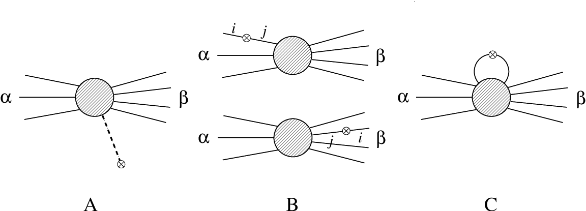
The first term has a pion pole term of the form

where $G_{\alpha\beta}^{\pi}(k)$ is the vertex function $\alpha\rightarrow\beta+\pi^{a}(k)$. For the on-shell pion at $k^{2}=0$, $G_{\alpha\beta}^{\pi}(k)$ reduces to the physical pion emission amplitude ${\cal M}(\alpha\rightarrow\beta+\pi^{a}(k))$ which we want to compute:

Therefore, if we use the current conservation law $k^{\mu}M_{\mu}^{a}(k)_{\alpha\beta}=0$, we can evaluate the pion emission amplitude indirectly from the other current matrix elements as

If we are interested in the soft limit $k\ \rightarrow\ 0$ of the amplitude, this implies that the only diagrams which have singularities at $k=0$ can contribute to such soft pion amplitudes.

Such singularities can generally appear if the current operator acts on the external one-particle lines as shown in the diagrams of category B in Fig. 1, whose amplitude is denoted by the second term ${\cal Q}_{\mu}^{a}(k)_{\alpha\beta}e^{-ikx}$. The rest diagrams in category C are regular at $k=0$ and cannot contribute. ${\cal Q}_{\mu}^{a}(k)_{\alpha\beta}e^{-ikx}$ has two contributions, one when the current is attached to the external line of the outgoing particle

and the other, when the current is attached to the external line of the initial particle

Here $\langle i|J_{\mu}^{a}(x)|j\rangle^{\rm ext}$ denotes the external line term ${\cal Q}_{\mu}^{a}(k)_{ij}e^{-ikx}$ for the single-particle case $\alpha=i$ and $\beta=j$, and $\alpha-i+j$ means that the particle $i$ in $\alpha$ is replaced by the particle $j$ with the same momentum $p_{i}=p_{j}$ on the mass-shell. It should be kept in mind that the ‘internal’ states $|j\rangle$ and $\langle j|$ here stand for slightly off-shell states before taking the soft limit $k\rightarrow 0$, and the expression

should be understood to be the propagator of the particle $j$ (so that the sum $\sum|j\rangle\langle j|$ over the polarization states gives the numerator of the propagator like, e.g., ${\vtop{\halign{#\cr\hfil/\hfil\crcr$p$\crcr}}}_{j}+m_{j}$ for the Dirac particle case.)

For the case where the particle $j$ is a massless gauge field, the numerator $\sum|j\rangle\langle j|$ contain not only the physical transverse states but also other unphysical polarization states. We will discuss this point more concretely in Sect.4.

These external line terms (2.13) and (2.14) contain propagators which have singularities $1/[(p_{i}\pm k)^{2}-m_{i}^{2}]=1/(\pm 2p_{i}\cdot k+k^{2})$ for on-shell momentum $p_{i}^{2}=m_{i}^{2}$.

Now we can apply the current conservation $k^{\mu}M_{\mu}^{a}(k)=0$ and take the limit $k\rightarrow 0$. From Eqs. (2.12) and (2.13), (2.14), we find

where $g_{A}^{a}(0)_{ij}$ is an ‘axial’ charge of the external line defined in [8]

This is the low-energy theorem for the single soft pion emission processes.

We emphasize here that we have only to evaluate the category B diagrams in which the current is attached to the external lines thanks to the current conservation. But we should note that this by no means implies that only the diagrams in which the pion couples to the external lines can contribute to the soft pion emission amplitude. Indeed there are generally diagrams in category A in which the pion (denoted by dotted line) is attached to the internal lines/vertices but which give non-vanishing amplitude in the soft limit.

The diagrams in category B possess the one-particle singularity so that the ‘charge’ $g_{A}^{a}(0)_{ij}$ is generically non-vanishing. However, in our ${\cal{N}}=8$ SG theory, no external lines can give non-vanishing $g_{A}^{a}(0)_{ij}$ charge so that all the single soft pion emission amplitudes vanish, as we will show below.

The classical non-gauge-fixed action of ${\cal{N}}=8$ SG has a gauge $SU(8)$ symmetry with antihermitian and traceless local parameters

and a global $E_{7(7)}$ symmetry with 133 parameters

In the $E_{7(7)}$ symmetry we have generators of the $SU(8)$ maximal subgroup of $E_{7(7)}$ with parameters $\Lambda_{I}{}^{J}$ and the orthogonal ones, in ${E_{7(7)}}/{SU(8)}$ with parameters $\Sigma^{MNPQ}$. There are 63 $\Lambda_{I}{}^{J}$ and they are antihermitian and traceless

They can be decomposed into 28 antisymmetric generators of the $SO(8)$ subgroup and 35 traceless symmetric generators orthogonal to $SO(8)$. If we write $\Lambda_{I}{}^{J}$ as the sum of the real and imaginary parts $\Lambda=\mbox{Re}\Lambda+i\,\mbox{Im}\Lambda$, then we have

where the real part is identified with the antisymmetric and the imaginary part with the symmetric part of $\Lambda$. The off-diagonal part has to satisfy the self-duality constraint with the phase $\eta=\pm 1$

We can also decompose $\Sigma$ into real and imaginary parts $\Sigma=\mbox{Re}\Sigma+i\,\mbox{Im}\Sigma$. However, in this case, both real and imaginary parts of $\Sigma$ have the same transposition properties

with $(\Sigma^{\mathsf{T}})_{IJKL}\equiv\Sigma_{KLIJ}$. Then the self-duality constraint implies that the real part is $\eta$-self-dual and imaginary part is $\eta$-anti-selfdual. The real and imaginary parts of $\Sigma$ each consists of 35 real parameters. Thus we present the 133 real parameters of $E_{7(7)}$ as $133=28+35+35+35$.

When the local $SU(8)$ symmetry is fixed in the unitary gauge as described in detail in [3], there are only 70 scalars (out of 133) left in ${G}/{H}={E_{7(7)}}/{SU(8)}$. The Noether current corresponding to $E_{7(7)}$ symmetry was presented in [3] based on the general Gaillard-Zumino procedure [9].

Here the 133 components of the current $J_{\mu}^{a}$ are contracted with the symmetry parameters $\epsilon_{a}$.

The $E_{7(7)}$-current is special since it corresponds to the symmetry of the equation of motion but not of the Lagrangian. This peculiarity appears in the point that the current $J^{\mu}$ can be given only if we use the dual vector field ${\cal B}_{\mu}$ which itself does not appear in the lagrangian and is a complicated non-local field if expressed in terms of the original fields, ${\cal A}_{\mu}$ and others.

That is, the current is given in the form as given by Gaillard and Zumino [9]:

where $\varphi_{i}$ stand for all the fields other than the vector field ${\cal A}_{\mu}$, and $\delta^{E}\!\varphi_{i}$ for the $E_{7(7)}$ transformation of $\varphi_{i}$. Here the $U(1)$ vector field strength $F$ and its dual $\tilde{F}$ are $F=d{\cal A}$ and $\tilde{F}_{\mu\nu}\equiv{1\over 2}\epsilon_{\mu\nu\rho\sigma}F^{\rho\sigma}$, and $\tilde{G}_{\mu\nu}$ is defined to be

and the parameter matrices $A,\,\cdots,\,D$ are given by

If the equation of motion $\partial_{\mu}\tilde{G}^{\mu\nu}=0$ is used, its dual $G_{\mu\nu}$ can be expressed as the field strength of the dual vector field $G=d{\cal B}$. Since $\tilde{G}^{\mu\nu}$ is defined by (3.26), $G=d{\cal B}$ is just an equation of motion.

We have suppressed here the internal indices on each vector field. In particular, in eq. (3.25) the first two indices of $\Sigma^{ijkl}$ are contracted with the left vector field strength ( $\tilde{G}$ or $\tilde{F}$ ) and the second two with the corresponding two indices of the vector field ( ${\cal A}$ or ${\cal B}$ ) on the right.

The 4-divergence of Eq. (3.25) gives

where we used $D^{\mathsf{T}}=-A$ in going to the last equality.

The problem here is the last term $\tilde{G}^{\mu\nu}BG_{\mu\nu}$, which cannot be written in a 4-divergence form unless we introduce the dual vector field ${\cal B}_{\mu}$, even if we use the equation of motion. Moreover, the Feynman rules in the presence of the dual vector field ${\cal B}_{\mu}$ are not available. This complicates the derivation of the low-energy theorem when this part of the current is used.

Therefore, from here on, we restrict to the current (and soft scalars) corresponding only to ${\rm Re}\Sigma$ of $E_{7(7)}/SU(8)$. We see from Eqs. (3.27) that only $A$ is non-vanishing and $B=C=0$ when $\Lambda={\rm Im}\Sigma=0$. Thus we have

The explicit form for the $E_{7(7)}$ current $j^{\mu}_{\varphi}$ was given in [3] and we will show the explicit forms for the quadratic in fields part below where we will need them.

We now examine the scattering amplitudes for the single pion emission processes (corresponding to ${\rm Re}\Sigma$).

Since the current $J^{\mu}$ is written solely in terms of the usual local fields for the ${\rm Re}\Sigma$ cases (no dual vectors), it is clear that only the singular diagrams for the current matrix element $\langle\alpha|J^{\mu}(x)|\beta\rangle$ could contribute to the soft-limit of the 4-divergence matrix element

Those are the category A and B diagrams. As explained in Sect.2, the pion emission amplitude given by the category A diagrams can be evaluated by the category B diagrams in which the current operator is inserted in the external lines.

We thus have only to evaluate the category B diagrams. For definiteness we consider the case where the soft pion is emitted with momentum $k$ from the external lines appearing in the final states, since the discussion for the initial state case is quite similar. Then we want to evaluate the external line part as shown in Fig. 2.

We call the external on-shell state field $\phi_{A}(p)$, and, looking back in time, it is converted by the current operator into a slightly off-shell particle $\phi_{B}(q)$ which propagates and connects to the source current $j_{B}$ in the main body of the diagram through the interaction Lagrangian $\phi_{B}j_{B}$. The external momentum $p$ and the pion momentum $k$ are put on the mass-shell $p^{2}=k^{2}=0$ and we work in the frame in which only $p^{+}$ and $k^{-}$ components are non-vanishing. Then the denominator of the slightly off-shell propagator becomes $q^{2}=(p+k)^{2}=2p\cdot k=2p^{+}k^{-}$.

Let us consider all case separately where those $\phi_{A}(p)$ and $\phi_{B}(q)$ stand for various possibilities of fields.

Before discussing the possibility of the higher-loop $E_{7(7)}(\mathbb{R})$ symmetry with 133 generators $X$ and $T$, let us remind that there are 70 generators of ${E_{7(7)}/SU(8)}$ symmetry, let us call them $X$, and there are 63 $T$-generators which form the maximal $SU(8)$ subalgebra. The total algebra consists of $[T,T]\sim T$ and $[X,T]\sim X$ and $[X,X]\sim T$. At the tree level for the amplitudes with any number of external states the following information has been obtained at present. On one hand, the studies in [10] and in [11] were performed directly on the amplitudes with an emission of a soft scalar and it has been established that all such tree amplitudes vanish in the soft limit. On the other hand, in this paper we have assumed that $E_{7(7)}(\mathbb{R})$ is preserved and studied the consequences of such assumption. One may argue that at the tree level the symmetry of the on-shell action cannot be anomalous and therefore it is not even an assumption that that $E_{7(7)}(\mathbb{R})$ is preserved in the form

for any matrix elements between physical states at the tree level. We have computed the amplitudes with an emission of a soft scalar associated with the term $(\partial^{\mu}J_{\mu}^{\rm lin})^{X}$ indirectly by computing the matrix elements of the second term $(\partial^{\mu}J_{\mu}^{\rm nonlin})^{X}$. This second term could have provided us with the relation between the soft amplitude with a scalar and the amplitudes without a scalar as shown in eq. (2.16): the relation between these two is given by the ‘axial’ charge [7, 8], which in our case is $g(0)_{ij}^{X}$. We have found that at the tree level in $\cal N$=8   SG all components of this charge are vanishing. Since at the tree level the conservation of the total Noether charge is taken for granted, $\partial^{\mu}J_{\mu}=0$, we have clearly an alternative derivation of the vanishing of soft amplitude with the emission of a boson. This follows from the $E_{7(7)}(\mathbb{R})$ symmetry. The subgroup $H=SU(8)$ of this symmetry just requires the current conservation and is not associated with any massless scalars

At higher loop level we have to assume that the total Noether charge is conserved, $\partial^{\mu}J_{\mu}$ both in the $SU(8)$ sector $T$ as well as in the coset part of it, $X$. From such an assumption in the $X$ part of the current we can only derive the low-energy theorem in the form of eq. (2.16). By itself it does not require that the soft limit of the amplitudes with a scalar should vanish: the symmetry only requires that the soft limit is defined via eq. (2.16) to be related to the amplitudes without a soft scalar times the ‘axial’ charge. One may entertain a scenario when at higher loops this charge is not vanishing, and the soft limit of the amplitudes with a scalar is also not vanishing. In such case the right hand side of equation (2.16) is equal to the left hand side, both non-vanishing, and we may still have an unbroken $E_{7(7)}(\mathbb{R})$ symmetry.

References

- [1] E. Cremmer and B. Julia, “The Supergravity Theory. 1. The Lagrangian,” Phys. Lett. B 80, 48 (1978); E. Cremmer, B. Julia and J. Scherk, “Supergravity theory in 11 dimensions,” Phys. Lett. B 76, 409 (1978); “The SO(8) Supergravity,” Nucl. Phys. B 159, 141 (1979).
- [2] B. de Wit and H. Nicolai, “ Supergravity,” Nucl. Phys. B 208, 323 (1982).
- [3] R. Kallosh and M. Soroush, “Explicit Action of on Supergravity Fields,” arXiv:0802.4106 [hep-th].
- [4] L. Brink, S. S. Kim and P. Ramond, “ on the Light Cone,” JHEP 0806, 034 (2008) [arXiv:0801.2993 [hep-th]].
- [5] S. L. Adler, “Consistency Conditions on the Strong Interactions implied by a Partially Conserved Axial-Vector Current. II,” Phys. Rev. 139, 1638 (1965); S. R. Coleman, “Secret Symmetry: An Introduction to Spontaneous Symmetry Breakdown and Gauge Fields,” in Aspects of Symmetry: Selected Erice Lectures by Sidney Coleman, CUP 1985.
- [6] S. Weinberg, “The Quantum Theory of Fields. Vol. 2: Modern Applications,” Cambridge, UK: Univ. Pr. (1996).
- [7] M. Bando, T. Kugo and K. Yamawaki, “Nonlinear Realization and Hidden Local Symmetries,” Phys. Rept. 164, 217 (1988).
- [8] T. Kugo and S. Uehara, “Massless Particle with Spin Implies the S-Matrix Symmetry” Prog. Theor. Phys. 66, 1044 (1981).
- [9] M. K. Gaillard and B. Zumino, “Duality Rotations for Interacting Fields,” Nucl. Phys. B 193, 221 (1981).
- [10] M. Bianchi, H. Elvang and D. Z. Freedman, “Generating Tree Amplitudes in SYM and SG,” arXiv:0805.0757 [hep-th].
- [11] N. Arkani-Hamed, F. Cachazo and J. Kaplan, “What is the Simplest Quantum Field Theory?,” arXiv:0808.1446 [hep-th].
- [12] A. K. Das and D. Z. Freedman, “Gauge Quantization for Spin 3/2 Fields,” Nucl. Phys. B 114, 271 (1976).
- [13] R. E. Kallosh, O. V. Tarasov and I. V. Tyutin, “One Loop Finiteness of Quantum Gravity off Mass Shell,” Nucl. Phys. B 137, 145 (1978).
- [14] C. M. Hull and P. K. Townsend, “Unity of Superstring Dualities,” Nucl. Phys. B 438, 109 (1995) [arXiv:hep-th/9410167].
- [15] E. Witten, “String Theory Dynamics in Various Dimensions,” Nucl. Phys. B 443, 85 (1995) [arXiv:hep-th/9503124].
- [16] M. B. Green, H. Ooguri and J. H. Schwarz, “Decoupling Supergravity from the Superstring,” Phys. Rev. Lett. 99, 041601 (2007) [arXiv:0704.0777 [hep-th]].
- [17] Z. Bern, J. J. Carrasco, L. J. Dixon, H. Johansson, D. A. Kosower and R. Roiban, “Three-Loop Superfiniteness of Supergravity,” Phys. Rev. Lett. 98, 161303 (2007) [arXiv:hep-th/0702112]; Z. Bern, J. J. M. Carrasco, L. J. Dixon, H. Johansson and R. Roiban, “Manifest Ultraviolet Behavior for the Three-Loop Four-Point Amplitude of Supergravity,” arXiv:0808.4112 [hep-th].
- [18] Z. Bern, L. J. Dixon and R. Roiban, “Is Supergravity Ultraviolet Finite?,” Phys. Lett. B 644, 265 (2007) [arXiv:hep-th/0611086]; M. B. Green, J. G. Russo and P. Vanhove, “Ultraviolet Properties of Maximal Supergravity,” Phys. Rev. Lett. 98, 131602 (2007) [arXiv:hep-th/0611273].
- [19] N. Marcus, “Composite Anomalies in Supergravity,” Phys. Lett. B 157, 383 (1985); P. di Vecchia, S. Ferrara and L. Girardello, “Anomalies Of Hidden Local Chiral Symmetries in Sigma Models and Extended Supergravities,” Phys. Lett. B 151, 199 (1985).