Cascades and Collapses, Great Walls and Forbidden Cities:
Infinite Towers of Metastable Vacua in Supersymmetric Field Theories

We shall begin the analysis of our models by focusing on a simple example: the $N=3$ special case, which consists of three $U(1)$ gauge groups and four chiral superfields. The scalar potential in this case is given by $V=V_{D}+V_{F}$, where

and

In these expressions, of course, $\phi_{i}$ denotes the (complex) scalar component of the chiral supermultiplet $\Phi_{i}$.

Given the scalar potential, it is then a straightforward matter to calculate the vacuum structure of this potential. Our results are as follows. Defining

we find that there are two (meta)stable vacua in this model for all $\lambda>\lambda_{3}^{\ast}$. The first vacuum state (which we shall call the $n=1$ vacuum) has energy $V_{1}=1/2$ and corresponds to the solution with

By contrast, the second vacuum state (which we shall call the $n=2$ vacuum) has vacuum energy $V_{2}={\textstyle{1\over 4}}(1-\chi)^{-1}$ and corresponds to the solution with

We thus see that the $n=1$ vacuum is of ${\bf\{{12}\}}$-type, while the $n=2$ vacuum is of ${\bf\{{13}\}}$-type. As emphasized above, both of these solutions are stable (without any flat or tachyonic directions) for all $\lambda>\lambda_{3}^{\ast}$; however, since $V_{1}>V_{2}$ for all $\chi<1/2$, we see that the $n=2$ vacuum is the true ground state in this theory, while the $n=1$ vacuum is only metastable. This vacuum configuration is sketched in Fig. 3.

Note that for $\lambda>\lambda_{3}^{\ast}$, the $n=1$ and $n=2$ vacua are separated by a potential barrier whose lowest point is a ${\bf\{{123}\}}$ saddle-point extremum of the scalar potential. Unlike the field-space solutions for the $n=1$ and $n=2$ vacua, which are $\lambda$-independent, the field-space solution for this saddle point depends quite strongly on $\lambda$. This is shown in Fig. 4, where the explicit solutions for $\{v_{1}^{2},v_{2}^{2},v_{3}^{2}\}$ are plotted for $\lambda>\lambda_{3}^{\ast}$.

It will be useful to understand how this vacuum structure deforms as a function of $\lambda$. Naïvely, one might suspect that taking $\lambda\to\infty$ would cause the height of this saddle-point barrier to diverge. However, we see from Fig. 4 that this is not the case: the scalar potential $V$ and all of the field VEV’s $v_{i}^{2}$ quickly reach finite asymptotes. Indeed, in the formal $\lambda\to\infty$ limit, we see that $v_{2}^{2},v_{3}^{2}\to 0$, whereupon our ${\bf\{{123}\}}$ saddle-point solution reduces to the ${\bf\{{1}\}}$ solution given by

with $V_{12}={\textstyle{1\over 2}}(1-\chi^{2})^{-1}$.

The above results are valid for all $\lambda>\lambda_{3}^{\ast}$. However, it will also be important for us to understand what happens as we reduce the value of $\lambda$ below $\lambda_{3}^{\ast}$. Since $\lambda$ sets the scale for the barrier height between the two vacua in Fig. 3, reducing $\lambda$ has the effect of reducing the barrier height between the two vacua. This in turn will destabilize our metastable vacuum. Specifically, we see from Fig. 4 that $\lambda_{3}^{\ast}\equiv 1/\sqrt{\chi(1+\chi)}$ is nothing but the critical value of $\lambda$ at which the barrier height becomes equal to $V_{1}$. At this critical value, the ${\bf\{{123}\}}$ saddle-point solution shown in Fig. 4 actually merges with the metastable $n=1$ vacuum solution (which is of ${\bf\{{12}\}}$-type) and thereby destabilizes it. Thus, as we take $\lambda$ below $\lambda_{3}^{\ast}$, we lose the $n=1$ vacuum. In order to emphasize that this is the critical $\lambda$-value at which the $n=1$ vacuum is destabilized, we shall also refer to $\lambda_{3}^{\ast}$ as $\lambda_{3,1}^{\ast}$.

Taking $\lambda$ still lower, we ultimately reach a second critical value $\lambda_{3,2}^{\ast}\equiv\sqrt{2/(2-\chi)}$ at which even the $n=2$ vacuum becomes destabilized. In this case, a new ${\bf\{{123}\}}$ solution becomes stable and serves as the ground state of the theory for all $\lambda<\lambda_{3,2}^{\ast}$.

These two critical values of $\lambda$ for the $N=3$ case are plotted in Fig. 5 as a function of the kinetic-mixing parameter $\chi$. Note, in particular, that $\lambda_{3,1}^{\ast}$ diverges as $\chi\to 0$. This shows that the stability of the $n=1$ metastable vacuum solution relies not only on having a sufficiently large value of $\lambda$, but also on the existence of non-zero kinetic mixing. Note also that

This indicates that as reduce $\lambda$ below $\lambda_{3}^{\ast}=\lambda_{3,1}^{\ast}$, our $N=3$ metastable “tower” destabilizes from the top down, with the $n=1$ metastable vacuum destabilizing before the $n=2$ vacuum. It is for this reason that we can associate $\lambda_{3}^{\ast}$ (the critical $\lambda$-value for stability for the entire tower) with $\lambda_{3,1}^{\ast}$ (the critical $\lambda$-value for stability of the highest vacuum).

We see, then, that our $N=3$ model gives rise to two vacuum solutions (one stable ground state and one metastable state above it) for all $\lambda>\lambda_{3}^{\ast}=\lambda_{3,1}^{\ast}$. The solutions for these vacua are $\lambda$-independent, and depend only on $\chi$. However, the barrier height between these two vacua (and hence the stability of the metastable vacuum) depends intimately on both $\chi$ and $\lambda$, and formally reaches an asymptote as $\lambda\to\infty$.

Having discussed the vacuum structure of the $N=3$ model, we now turn to the $N=4$ model. In this case, there are four $U(1)$ gauge groups and five chiral superfields. Defining

we find that the vacuum structure now consists of three vacuum solutions, each without tachyonic or flat directions, for all $\lambda>\lambda_{4}^{\ast}$. The $n=1$ vacuum has energy $V_{1}=1/2$, just as in the $N=3$ case, and corresponds to the solution with

while the $n=2$ vacuum has energy $V={\textstyle{1\over 4}}(1-\chi)^{-1}$, again just as in the $N=3$ case, and now corresponds to the solution with

The solutions in Eqs. (20) and (21) are clearly the $N=4$ generalizations of the corresponding $N=3$ solutions in Eqs. (15) and (16) respectively. However, the crucial new feature for the $N=4$ case is the appearance of an additional vacuum state of even lower energy. This vacuum state, which we shall refer to as the $n=3$ vacuum, has energy $V_{3}={\textstyle{1\over 2}}(3-4\chi)^{-1}$ and corresponds to the solution with

This vacuum structure is sketched in Fig. 6. Note that just as in the $N=3$ case, these vacuum solutions are all $\lambda$-independent.

For $\lambda>\lambda_{4}^{\ast}$, the $n=1$, $n=2$, and $n=3$ vacua are separated by potential barriers whose lowest points are all ${\bf\{{1234}\}}$ saddle-point extrema of the scalar potential. Unlike the field-space solutions for the (meta)stable vacua, the field-space solutions for these saddle points depend quite strongly on $\lambda$. However, in the formal $\lambda\to\infty$ limit, these solutions all quickly reach finite asymptotes. For example, the asymptotic saddle-point solution between the $n=1$ and $n=2$ vacua is of ${\bf\{{12}\}}$-type and is given by

with energy $V_{12}={\textstyle{1\over 2}}(1-\chi^{2})^{-1}$. This is the $N=4$ analogue of the $N=3$ asymptotic saddle-point solution in Eq. (17), and continues to have the same energy $V_{12}$. However, in the $N=4$ case there are also additional saddle-point solutions which involve the new $n=3$ vacuum. Specifically, the asymptotic saddle-point solution which lies directly between the $n=1$ and $n=3$ vacua is of ${\bf\{{13}\}}$-type and is given by

with energy $V_{13}=(1-\chi)/(2-2\chi-\chi^{2})$, while the asymptotic saddle-point solution between the $n=2$ and $n=3$ vacua is of ${\bf\{{14}\}}$-type and is given by

with energy $V_{23}={\textstyle{1\over 2}}(2-2\chi-\chi^{2})^{-1}$.

This vacuum structure emerges for all $\lambda>\lambda_{4}^{\ast}$. However, just as in the $N=3$ case, we find that reducing $\lambda$ below $\lambda_{4}^{\ast}$ tends to destabilize our vacuum tower. Specifically, one finds that there are now three critical $\lambda$-values, denoted $\lambda_{4,1}^{\ast}$, $\lambda_{4,2}^{\ast}$, and $\lambda_{4,3}^{\ast}$, at which the $n=1$, $n=2$, and $n=3$ vacua are respectively destabilized. These three critical values are given by

and all three are plotted in Fig. 7 as functions of $\chi$. We see from this figure that

for all $0<\chi<1/2$. This implies that just as in the $N=3$ case, our vacuum tower destabilizes from the top down as we reduce $\lambda$ below $\lambda_{4,1}^{\ast}$. As a result of Eq. (27), we see that $\lambda_{4}^{\ast}$ (i.e., the critical $\lambda$-value for stabilizing the entire $N=4$ vacuum tower) is nothing but $\lambda_{4,1}^{\ast}$ (the maximum of the individual values $\lambda_{4,n}^{\ast}$ for stabilizing any of the individual vacua in the tower). It is this observation which underlies the identification given in Eq. (19). We also observe from Fig. 7 that non-zero kinetic mixing is also required in order for the stability of our metastable vacua.

It is clear that the $N=4$ case is a direct generalization of the $N=3$ case. Once again, the vacuum solutions are $\lambda$-independent, while the barrier heights (and hence the stability of these vacuum solutions) are $\lambda$-dependent. Moreover, the energies associated with the $n=1$ and $n=2$ vacua, as well as the barrier between them, are unchanged in passing from the $N=3$ case to the $N=4$ case. Indeed, the primary new feature in passing from the $N=3$ case to the $N=4$ case is the emergence of a new vacuum solution, our so-called $n=3$ vacuum, which “slides in” below the previous bottom of the tower and becomes the new ground state of the theory for all $\lambda>\lambda_{4,3}^{\ast}$. As a result, our previous $n=2$ ground state in the $N=3$ theory now becomes the first-excited metastable state in the $N=4$ theory, and our tower of metastable vacua has grown by one additional metastable vacuum. We stress again that all of these vacua are either strictly stable or strictly metastable. In particular, they contain neither tachyonic masses nor flat directions.

We now turn to the case with general $N$. As might be expected, the pattern we have seen in passing from the $N=3$ case to the $N=4$ case continues without major alteration. For general $N$ and for $\lambda$ exceeding a critical value $\lambda_{N}^{\ast}$, we find that our model has a vacuum structure consisting of a tower of $N-1$ stable vacua: a single stable ground state, and $N-2$ metastable vacua above it. As in the $N=3$ and $N=4$ cases discussed above, we shall number these vacua from the top down with an index $n$, so that the $n=1$ vacuum sits at the top of the tower and the $n=N-1$ vacuum (the true ground state of the theory) sits at the bottom.

We then find that the $n$-vacuum has energy

where

and corresponds to the solution with

As evident from these VEV’s, this is clearly a solution of ${\bf\{{1,...,N-n,N-n+2,...,N}\}}$-type. It is easy to verify that these results reduce to those already quoted for the $N=3$ and $N=4$ special cases. Note that the vacuum energies $V_{n}$ along the tower are independent of $N$, as expected; indeed, all that depends on $N$ are the number of such vacua and their precise field VEV’s. Also note that $V_{N-1}\to 0$ as $N\to\infty$.

As in the previous special cases with $N=3$ and $N=4$, any two vacua $n$ and $n^{\prime}$ are separated by a saddle-point solution. In the formal $\lambda\to\infty$ limit, we find that this barrier height asymptotes to the value

where $R_{n}$ is defined in Eq. (29) and where we have taken $n^{\prime}>n$. Note that $V_{nn^{\prime}}$ is also independent of $N$. The corresponding asymptotic saddle-point solutions are given by

These results are plotted in Fig. 8 for the $N=20$ model. Clearly, the vacuum structure of this model consists of a ground-state vacuum along with a tower of 18 metastable vacua above it. In Fig. 8, we have shown the vacuum energies of these vacua, along with the asymptotic energies of the saddle-point barriers which connect “nearest-neighbor” vacua, as functions of a cumulative distance in field space along a path that winds through each vacuum configuration and over each saddle point as it comes down the tower, vacuum by vacuum. In essence, then, this figure forms a linear “picture” of the tower.

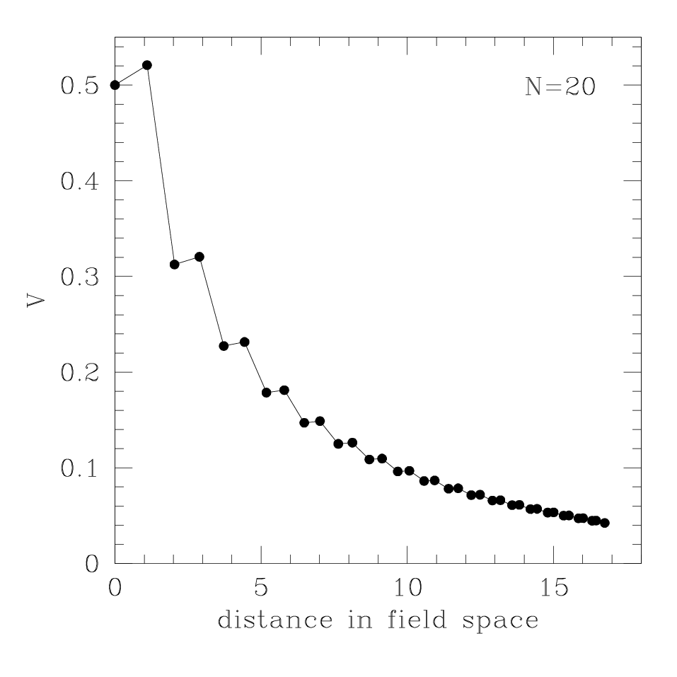
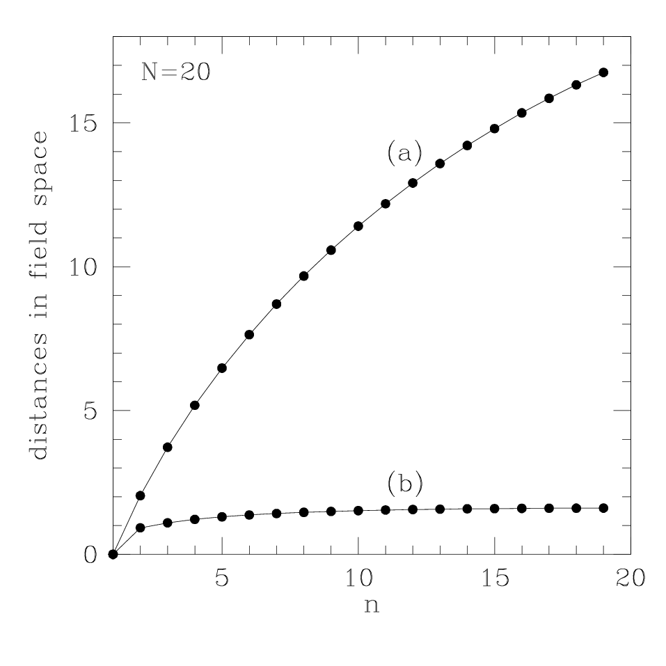
Despite the relative simplicity of Fig. 8, it is worth emphasizing that the geometry of the metastable vacuum tower in the full $(N+1)$-dimensional field space is rather non-trivial. For example, although the vacuum and saddle-point energies are plotted in Fig. 8 versus a cumulative, integrated distance as we wind our way down the vacuum tower, we could have just as easily defined the field-space distance associated with any vacuum or saddle point in terms of its straight-line distance directly back to a reference vacuum (such as the $n=1$ vacuum at the top of the tower). The difference between these two different notions of distance is shown in Fig. 9 for the $N=20$ case. Indeed, as evident from the actual solutions given Eq. (30), the vacua in our vacuum tower actually lie along a “spiral” or “helix” in the $N$-dimensional $v_{N+1}=0$ subspace of our full $(N+1)$-dimensional field space.

It is also important to emphasize that Fig. 8 shows only those saddle-point barriers which exist between nearest-neighbor vacua along the vacuum tower. In actuality, however, there are saddle-point barriers which exist directly between any two vacua $(n,n^{\prime})$. As a result, it is possible to imagine descending through the vacuum tower taking “hops” with different values of $\Delta n$ at each step. Fig. 10 provides an illustration of the effects of different possiblities.

Finally, we turn to the one remaining issue: the critical value $\lambda_{N,n}^{\ast}$ at which the $n^{\rm th}$ vacuum in the tower is destabilized. In general, for any $N\geq 2$ and $1\leq n\leq N-1$, it turns out that $\lambda_{N,n}^{\ast}$ is given by

where $y\equiv\chi/(1-2\chi)=n/(R_{n}-2)$ and where $\Gamma(z)$ is the Euler $\Gamma$-function [for which $\Gamma(z)=(z-1)!$ when $z\in\mathchoice{\hbox{\cmss Z\kern-3.99994ptZ}}{\hbox{\cmss Z\kern-3.99994ptZ}}{\lower 0.9pt\hbox{\cmsss Z\kern-2.79996ptZ}}{\lower 1.2pt\hbox{\cmsss Z\kern-2.79996ptZ}}^{+}$]. It is straightforward to verify that these expressions reduce to the corresponding expressions for the $N=3$ and $N=4$ cases plotted in Figs. 5 and 7 respectively. For example, using the result in Eq. (33), we find that

In Fig. 12, we plot the values of $\lambda_{N,n}^{\ast}$ as functions of $\chi$ for $N=20$ and $1\leq n\leq 19$. Unlike the simpler $N=3$ and $N=4$ cases, however, we see that it is no longer true that $\lambda_{N,n}^{\ast}>\lambda_{N,n^{\prime}}^{\ast}$ for any $n<n^{\prime}$. Instead, as $N$ increases, we see that a complicated “crossing” pattern develops as a function of $\chi$. As a result of this crossing pattern, the value of $n$ which results in the maximum value of $\lambda_{N,n}^{\ast}$ itself varies with $\chi$, as shown in Fig. 12. Nevertheless, for any value of $\chi$, we see that our entire vacuum tower will be stable if $\lambda>\lambda_{N}^{\ast}$, where

Thus, $\lambda_{N}^{\ast}$ corresponds to the upper “envelope” of the curves shown in Fig. 12.

The crossing pattern shown in Fig. 12 implies that our tower of metastable vacua will experience a non-trivial destabilization pattern as $\lambda$ is reduced from infinity. For any value of $\chi$ in the range $0<\chi<1/2$, the first vacuum to be destabilized is indicated in Fig. 12. This serves as the initial destabilization point on the tower. Reducing $\lambda$ still further then induces a destabilization of the vacua immediately above and below this point, and further reductions in $\lambda$ result in a destabilization “wave” which simultaneously runs both up and down the vacuum tower from this initial point until ultimately all vacua are destabilized.

Finally, the dependence of $\lambda_{N}^{\ast}$ on $N$ is shown in Fig. 13. We see that $\lambda_{N}^{\ast}$ generally grows rather quickly with $N$. Moreover, as already anticipated from the $N=3$ and $N=4$ special cases, $\lambda_{N}^{\ast}$ always diverges as $\chi\to 0$ and asymptotes to $\lambda_{N}^{\ast}\to\sqrt{2^{N-1}/3}$ as $\chi\to 1/2$. The fact that $\lambda_{N}^{\ast}$ diverges as $\chi\to 0$ for every $N$ indicates that kinetic mixing plays a critical role in keeping our metastable vacuum tower stable.

We also stress that the $\lambda$-values plotted in Fig. 13 are the rescaled, dimensionless versions of our original Wilson-line coefficients. Indeed, they are only rescaled variables, not to be confused with our primordial Lagrangian couplings; indeed, as discussed earlier, this rescaling absorbs powers of the underlying gauge coupling $g$ and the Fayet-Iliopoulos coefficient $\xi$. This rescaling is thus partly responsible for the rise in $\lambda_{N}^{\ast}$ as a function of $N$. However, having such large values of $\lambda$ naturally begs the question as to whether the stability of our vacuum towers is in conflict with the assumed perturbativity of our model. However, as we shall see below, there is no conflict between the two, and indeed such large values of the rescaled $\lambda$ do not in and of themselves undermine the validity of our tree-level calculations.

The results obtained thus far have rested on the assumption that the physics of our model is perturbative at all relevant scales and is therefore accurately approximated by tree-level calculations. However, the true vacua of our theory are those field configurations which minimize the full effective potential $V_{\mathrm{eff}}(\phi_{i})$, and this includes radiative corrections. Thus, the tower of metastable vacua which we have presented above is guaranteed to be an accurate description of the actual vacuum structure of our model if and only if such corrections are small and $V_{\mathrm{eff}}(\phi_{i})\approx V_{\mathrm{tree}}$, with $V_{\mathrm{tree}}$ given in Eq. (8). Indeed, this must hold within the vicinity of the solution to the classical potential for each applicable vacuum index $n$.

We will now demonstrate that there is no problem satisfying all applicable perturbativity constraints, provided the gauge coupling $g$ is taken to be sufficiently small. Moreover, since small $g$ is also beneficial for stabilizing the vacua in the tower, we shall find that there is no conflict between the constraints stemming from perturbativity and those stemming from vacuum stability — even as $N\to\infty$.

Note that in this subsection only, we shall revert back to our original unrescaled dimensionful parameters in order to expose the explicit dependence of our physical quantities on the gauge coupling $g$. This will restore factors of $g$ and $\xi$ in many of our previous expressions. For example, in terms of the original unrescaled dimensionful quantities $\lambda$ and $\xi$, our expression for $\lambda_{N,n}^{\ast}$ in Eq. (33) takes the form

Similar modifications to other expressions occur as well.

It turns out that a great deal of information about the effective potential can be gleaned from non-renormalization theorems [15]. For example, in supersymmetric field theories, the superpotential is not renormalized by perturbative effects, except via wavefunction renormalization. Moreover, this holds true even when the superpotential includes non-renormalizable operators [16]. As a result of such theorems, we expect corrections to $V_{F}$ to arise only at scales near or below the supersymmetry-breaking scale $g\sqrt{\xi}$. However, these are typically the energy scales in which we are interested. Moreover, corrections to the Kähler potential do not, in general, vanish in supersymmetric theories. Thus, it will be necessary to discuss both sorts of corrections.

We begin by addressing radiative corrections to the Kähler potential. These arise due to diagrams which contribute to wavefunction renormalization of the various fields in the theory, and depend on $g$. For our purposes, it will be sufficient to focus on one-loop radiative corrections to the $\phi_{i}$ propagator; the contributing diagrams are then shown in Fig. 14. Let us begin by considering the contribution from diagrams with scalars running in the loop. There are $N+1$ such diagrams, and they result in a net contribution

where $m_{j}$ is the mass of $\phi_{j}$, where $\mu$ is an arbitrary renormalization scale, and where

If $T_{ij}$ were an arbitrary matrix, the expression in Eq. (37) would scale roughly as $N+1$ for large $N$, and the theory would rapidly become non-perturbative.

This is not the case, however, due to certain properties of $T_{ij}$ which are essentially consequences of the moose structure of the model. In particular, all entries along the diagonal of this matrix are positive and $\mathcal{O}(1)$. Likewise, all elements with $i\neq j$ satisfy $-1<T_{ij}<0$, and the sum of elements in any row or column of $T$ vanishes. Together, these properties imply that the contribution to the renormalization of the Kähler potential from scalar loops is essentially independent of $N$. Moreover, each of the additional diagrams in Fig. 14 yields a contribution to the two-point function for $\phi_{i}$ which is roughly of the order of $T_{ii}$ (no sum on $i$). This is also essentially independent of $N$. Consequently, the renormalization of the Kähler potential is under control, and radiative corrections of this sort can be safely neglected as long as $g\ll 4\pi$ — even for very large $N$.

The second class of diagrams we must consider are corrections to the $2N$-field couplings in $V_{F}$ which come from the terms in $V_{D}$. In other words, these are corrections to the superpotential coupling $\lambda$ which arise from non-zero $g$. The leading such contribution arises at one-loop order from diagrams of the sort depicted in Fig. 15, along with additional diagrams in which gauge bosons and gauginos run in the loop. Note that similar diagrams were examined in Ref. [17]. In the limit of unbroken supersymmetry, of course, these contributions would sum to zero.

Each of the contributing diagrams of the sort pictured in Fig. 15 contains $N$ vertices, and each of these vertices contributes a factor of $g^{2}T_{ij}$ as well as $N$ scalar propagators. In any $n$-vacuum, the scalar masses are expected to be $\sim\mathcal{O}(g^{2}\xi R_{n}^{-1})$, so each diagram is proportional to $g^{2}$. There are $N!\sim N^{N}$ such diagrams, but each is proportional to $\mathrm{Tr}[T_{i_{1}i_{2}}T_{i_{2}i_{3}}\ldots T_{i_{N-1}T_{N}}]$ and hence suppressed by a factor of $T_{ij}^{N}\sim(1/N)^{N}$, where $i\neq j$. Thus, as was the case with the wavefunction-renormalization calculation above, the $N$-dependence essentially cancels. Thus, as long as $g\ll 4\pi$, this contribution too can be neglected — regardless of the value of $N$. By the same token, contributions to other effective operators which involve couplings of various numbers of scalar fields can also be safely neglected.

The final category of radiative corrections we must consider are corrections to the effective $2N$-scalar couplings, each of which has the tree-level coefficient $\lambda^{2}$. Thus, these are essentially corrections to the superpotential coefficient $\lambda$ which themselves depend on $\lambda$. The leading contribution arises at one-loop order from diagrams of the form shown in Fig. 17, in which $2N-4$ fields are replaced by their VEV’s, chosen appropriately for a given vacuum. However, along with these contributions we must also include the contributions from diagrams of the form shown in Fig. 17, also with VEV’s assigned to an appropriate number of external fields. Again, these contributions cancel in the limit of unbroken supersymmetry, but their contributions can be expected to survive below the supersymmetry-breaking scale.

In the $n$-vacuum, the one-loop contribution to the $(\prod_{i=1}^{N+1}|\phi|^{2})/|\phi_{\ell}|^{2}$ vertex from a given diagram of the sort shown in Fig. 17 is roughly

References

- [1] J. R. Ellis, C. H. Llewellyn Smith and G. G. Ross, Phys. Lett. B 114, 227 (1982); M. Dine and A. E. Nelson, Phys. Rev. D 48, 1277 (1993) [arXiv:hep-ph/9303230]; M. Dine, A. E. Nelson, Y. Nir and Y. Shirman, Phys. Rev. D 53, 2658 (1996) [arXiv:hep-ph/9507378]; S. Dimopoulos, G. R. Dvali, R. Rattazzi and G. F. Giudice, Nucl. Phys. B 510, 12 (1998) [arXiv:hep-ph/9705307]; M. A. Luty, Phys. Lett. B 414, 71 (1997) [arXiv:hep-ph/9706554]; M. A. Luty and J. Terning, Phys. Rev. D 62, 075006 (2000) [arXiv:hep-ph/9812290].
- [2] K. Intriligator, N. Seiberg and D. Shih, JHEP 0604, 021 (2006) [arXiv:hep-th/0602239]; JHEP 0707, 017 (2007) [arXiv:hep-th/0703281].
- [3] R. Bousso and J. Polchinski, JHEP 0006, 006 (2000) [arXiv:hep-th/0004134]; J. L. Feng, J. March-Russell, S. Sethi and F. Wilczek, Nucl. Phys. B 602, 307 (2001) [arXiv:hep-th/0005276].
- [4] T. Banks, M. Dine and L. Motl, JHEP 0101, 031 (2001) [arXiv:hep-th/0007206].
- [5] G. L. Kane, M. J. Perry and A. N. Zytkow, arXiv:hep-th/0311152.
- [6] See, e.g., S. H. H. Tye, arXiv:hep-th/0611148; arXiv:0708.4374 [hep-th]; S. Sarangi, G. Shiu and B. Shlaer, arXiv:0708.4375 [hep-th].
- [7] S. S. Haque, G. Shiu, B. Underwood and T. Van Riet, arXiv:0810.5328 [hep-th].
- [8] K. R. Dienes and B. Thomas, to appear.
- [9] M. B. Green and J. H. Schwarz, Phys. Lett. B 149, 117 (1984).
- [10] E. Dudas, A. Falkowski and S. Pokorski, Phys. Lett. B 568, 281 (2003) [arXiv:hep-th/0303155].
- [11] B. Holdom, Phys. Lett. B 166, 196 (1986).
- [12] K. R. Dienes, C. F. Kolda and J. March-Russell, Nucl. Phys. B 492, 104 (1997) [arXiv:hep-ph/9610479].
- [13] K. R. Dienes, E. Dudas and T. Gherghetta, Phys. Rev. D 72, 026005 (2005) [arXiv:hep-th/0412185].
- [14] K. R. Dienes and B. Thomas, Phys. Rev. D 78, 106011 (2008) [arXiv:0806.3364 [hep-th]].
- [15] M. T. Grisaru, W. Siegel and M. Rocek, Nucl. Phys. B 159, 429 (1979).
- [16] S. Weinberg, Phys. Rev. Lett. 80, 3702 (1998) [arXiv:hep-th/9803099].
- [17] A. Falkowski, C. Grojean and S. Pokorski, Phys. Lett. B 581, 236 (2004) [arXiv:hep-ph/0310201].
- [18] U. van Kolck, Nucl. Phys. A 645, 273 (1999) [arXiv:nucl-th/9808007]; P. F. Bedaque and U. van Kolck, Ann. Rev. Nucl. Part. Sci. 52, 339 (2002) [arXiv:nucl-th/0203055].
- [19] S. R. Coleman, Phys. Rev. D 15, 2929 (1977) [Erratum-ibid. D 16, 1248 (1977)]; C. G. . Callan and S. R. Coleman, Phys. Rev. D 16, 1762 (1977).
- [20] M. J. Duncan and L. G. Jensen, Phys. Lett. B 291, 109 (1992).
- [21] S. A. Abel, C. S. Chu, J. Jaeckel and V. V. Khoze, JHEP 0701, 089 (2007) [arXiv:hep-th/0610334]; N. J. Craig, P. J. Fox and J. G. Wacker, Phys. Rev. D 75, 085006 (2007) [arXiv:hep-th/0611006]; W. Fischler, V. Kaplunovsky, C. Krishnan, L. Mannelli and M. A. C. Torres, JHEP 0703, 107 (2007) [arXiv:hep-th/0611018].
- [22] N. Arkani-Hamed, A. G. Cohen and H. Georgi, Phys. Rev. Lett. 86, 4757 (2001) [arXiv:hep-th/0104005]; C. T. Hill, S. Pokorski and J. Wang, Phys. Rev. D 64, 105005 (2001) [arXiv:hep-th/0104035].
- [23] K. Sfetsos, Nucl. Phys. B 612, 191 (2001) [arXiv:hep-th/0106126]; H. Abe, T. Kobayashi, N. Maru and K. Yoshioka, Phys. Rev. D 67, 045019 (2003) [arXiv:hep-ph/0205344]; L. Randall, Y. Shadmi and N. Weiner, JHEP 0301, 055 (2003) [arXiv:hep-th/0208120].
- [24] Z. Lalak and O. J. Eyton-Williams, arXiv:0807.4120.
- [25] J. D. Brown and C. Teitelboim, Phys. Lett. B 195, 177 (1987).
- [26] M. R. Douglas, JHEP 0305, 046 (2003) [arXiv:hep-th/0303194].
- [27] L. Susskind, arXiv:hep-th/0302219.
- [28] H. B. Nielsen and P. Olesen, Nucl. Phys. B 61 (1973) 45; T. W. B. Kibble, J. Phys. A 9, 1387 (1976).
- [29] http://en.wikipedia.org/wiki/The_Red_Wheelbarrow