Exciton-exciton interaction and biexciton formation in bilayer systems
Abstract
We report quantum Monte Carlo calculations of biexciton binding energies in ideal two-dimensional bilayer systems with isotropic electron and hole masses. We have also calculated exciton-exciton interaction potentials, and pair distribution functions for electrons and holes in bound biexcitons. Comparing our data with results obtained in a recent study using a model exciton-exciton potential [C. Schindler and R. Zimmermann, Phys. Rev. B 78, 045313 (2008)], we find a somewhat larger range of layer separations at which biexcitons are stable. We find that individual excitons retain their identity in bound biexcitons for large layer separations.
pacs
71.35.Cc, 78.67.De, 02.70.SsI Introduction
Electrons and holes in semiconductors can combine to form hydrogen-like bound states called excitons. The creation and recombination of excitons is one of the principal mechanisms by which light interacts with semiconductors. Furthermore, excitonic systems possess a number of unusual properties, such as the ability to transport energy without transporting charge, suggesting a range of applications in novel electronic devices. Excitonic systems have therefore been the subject of numerous experimental[1, 2, 3, 4, 5] and theoretical[6, 7, 8] studies in recent years.
In the low-density limit, excitons may be regarded as weakly-interacting neutral bosons.[3] Bose-Einstein condensation of excitons is therefore possible. However, it has proved to be difficult to obtain exciton lifetimes that are sufficiently long for thermalization to take place, and the current experimental evidence for Bose-Einstein condensation is inconclusive.[9, 10] One promising approach for overcoming the problem of short lifetimes is the development of coupled-quantum-well (bilayer) systems, in which thin layers of semiconductor and an applied electric field in the growth direction are used to confine the electrons and holes to spatially separated, parallel, quasi-two-dimensional wells, hindering recombination and extending exciton lifetimes.[2, 1, 5]
At present our understanding of the exciton-exciton interaction in bilayer systems is limited. On the one hand there is a repulsive electrostatic interaction between excitons. For example, if the layer separation is nonzero then the excitons have parallel dipole moments, giving an asymptotically dominant repulsive interaction. Furthermore, the static charge distribution of each exciton has a permanent quadrupole moment in general (even at zero layer separation, provided the electron and hole masses differ), giving another repulsive interaction term.[8] On the other hand, fluctuating dipole (van der Waals) forces result in an attraction between excitons at short range. Because of the existence of the van der Waals forces, it is sometimes possible for biexcitons (bound states of pairs of excitons) to form. A better understanding of the interaction between excitons in coupled quantum wells will facilitate the interpretation of experimental data, in particular enabling the determination of the exciton densities achieved in experiments.
The dependence of exciton and biexciton binding energies on the layer separation has been investigated by Tan et al., who found that, while the exciton binding energy decays slowly as the inverse of the layer separation, the biexciton binding energy decays extremely rapidly.[7] Recent studies of the exciton-exciton interaction using a heavy-hole approximation have found there to be a critical layer separation for each electron/hole mass ratio, beyond which biexcitons become unstable with respect to dissociation into two separate excitons.[11, 8] In this article we report quantum Monte Carlo (QMC) calculations of the binding energies of biexcitons in bilayer systems and exciton-exciton interaction potentials.
The rest of this article is arranged as follows. In Sec. II we describe our calculations of the binding energies of biexcitons and investigate the range of layer separations and mass ratios for which biexcitons are stable. In Sec. III we present our data for the exciton-exciton interaction potential. In Sec. IV we report pair-distribution functions (PDF’s) for biexcitons. Finally, we draw our conclusions in Sec. V. We use Hartree atomic units () throughout this article, although we report final energies in exciton Rydbergs (, where is the reduced mass of an exciton and and are the electron and hole masses) and lengths in terms of exciton Bohr radii [].
II Biexciton binding energies
We have modeled the coupled-quantum-well system by an idealized two-dimensional (2D) bilayer, in which the electrons and holes are confined to two parallel planes, and the effective mass tensors of the electrons and holes are isotropic. In reality, electrons and holes are free to move within quantum wells that are of finite width (e.g., one experimental setup[3] has well widths of 8 nm and a well separation of 4 nm), although the Coulomb attraction between electrons and holes should keep the particles confined to the inner edges of their respective wells. We have also restricted our attention to biexciton systems in which the two electrons have opposite spins, as do the two holes, because this is the ground-state spin configuration.
We have studied biexcitons and exciton-exciton interactions using the variational and diffusion quantum Monte Carlo (VMC and DMC) methods. In the VMC method the expectation value of the Hamiltonian with respect to a trial wave function is calculated using a stochastic integration technique.[12] Trial wave functions usually contain a number of free parameters, to be optimized by minimizing either the energy expectation value or the variance of the energy. DMC is a stochastic projector technique for solving the many-body Schrödinger equation.[13, 12] DMC is in principle exact for systems with nodeless ground-state wave functions, such as the biexciton systems studied in this work.
Our trial wave function was similar to that of Tan et al.,[7] with additional flexibility provided by multiplication by a two-body Jastrow factor.[14] This wave function satisfies the Kato cusp conditions when particles coincide,[15] and reduces to the form appropriate for two isolated excitons when the excitons are far apart. We also carried out some calculations using a three-body Jastrow factor.[16] For a typical case where , the reduction in the VMC energy from the inclusion of a three-body term was . Obtaining the best possible trial wave function was especially important for the PDF calculations described in Sec. IV.
We optimized the free parameters in our wave function by unreweighted variance minimization[17, 18, 19] and linear-least-squares energy minimization.[20] The trial wave function can describe the dissociated system more accurately than it can describe the bound system; hence energy minimization is the more sensible choice for investigating binding, although this depends upon initial parameters and configurations. Although the DMC energy is independent of the trial wave function, the statistical efficiency of the method is increased when the wave function is improved. By using a more flexible wave function, we have been able to achieve considerably smaller error bars than Tan et al.[7] All the QMC calculations reported in this article were performed using the casino program.[16]
For each layer separation and electron/hole mass ratio , the biexciton binding energy was calculated as , where is the energy of a single exciton and is the energy of the four-body biexciton system. The exciton energy was obtained using a numerically exact Runge-Kutta integration technique as described in Ref. 7, while DMC was used to calculate the biexciton energy . The DMC energies were converged with respect to time step and population size; any remaining bias is much smaller than the statistical error bars.
Biexciton binding energies for , , and are shown in Figs. 1, 2, and 3, respectively. It can be seen that our results are close to those of Tan et al.;[7] the difference arises from our use of exact single-exciton energies. Tan et al. used Eq. (3) of Ref. 7 to generate values, introducing a small, systematic error. Removing this error reveals that our DMC data are in statistical agreement with those of Tan et al. The random errors in our data are much smaller, so we can locate the layer separation at which the biexciton ceases to be bound. Tan et al. fitted an exponential form to their binding energy data, which resulted in the erroneous conclusion that biexciton binding persists to infinite layer separation.
Our DMC results show some deviation from the binding energies obtained by Schindler and Zimmermann,[8] especially when , when , and when the mass ratio is close to 1, because we have performed a full simulation of all four particles in the biexciton, whereas they simulated a pair of excitons interacting via a model potential. The deviation of our binding energies from those of Schindler and Zimmermann is approximately where . At smaller the agreement is much better, but below we find larger differences, reaching a maximum of almost at , as shown in Figs. 1 and 2.
As can be seen in Fig. 4, which shows the range of and over which the biexciton is stable, we find a somewhat larger region of stability for the biexciton than Schindler and Zimmermann. Let be the critical layer separation, beyond which the biexciton is unbound. As , the heavy-hole approximation made by Schindler and Zimmermann becomes increasingly accurate, and our results for agree with theirs. On the other hand, for their interaction potential is less accurate and our value of is therefore significantly higher than theirs.
Our data are mostly in excellent agreement with those of Meyertholen and Fogler, although at small we find a slightly larger region of biexciton stability. This is not an artifact of the extrapolation, which followed the scheme set out in Ref. 21, for we were able to find points with nonzero binding energies outside the region of stability defined by Meyertholen and Fogler. This is consistent with the variational principle that applies to their results.
One may parameterize the boundary of the region of biexciton stability in Fig. 4. Expressing in terms of ensures that the correct behavior is observed upon exchanging the electron and hole masses [i.e., ]. A suitable fitting function is
| (1) |
where the parameter values and give a error of per data point. The functional form of Eq. (1) satisfies most of the conditions derived in Ref. 21: is infinite, and for .


III Exciton-exciton interaction
The exciton-exciton interaction potential at separation is defined to be the energy of a biexciton system in which the centers of mass of the two excitons are constrained to be a distance apart, minus the energies of two isolated excitons. The Hamiltonian for the constrained biexciton system may be written as
where and are the electron-hole separations within the two excitons. The first two potential terms represent the intra-exciton electron-hole potentials, followed by the hole-hole, electron-electron, and finally the two inter-exciton electron-hole terms. DMC calculations can then be performed for an effective two-particle system, with coordinates and . The kinetic-energy operator only includes derivatives with respect to in-plane coordinates. The form of trial wave function was the same as that used in Sec. II, but with the electron and hole coordinates being re-expressed in terms of , , and the fixed vector .
The center-of-mass constraint may not be used to calculate the interaction potential at zero exciton-exciton separation, because in that limit the repulsion becomes strong enough to dissociate the two individual excitons. The ground state of Eq. () at very small is thus not the physical quantity we require. We have calculated the exciton-exciton potential only at separations for which the excitons remain bound. Figure 5 demonstrates this effect, exhibiting a potential which decreases at small to physically unreasonable values.
Our DMC calculations yield a smooth exciton-exciton potential. The interaction energies shown in Fig. 5 do not deviate from simple dipole-dipole repulsion of the form
| (3) |
by more than above an exciton-exciton separation of . The fits to the interaction potential data are shown in Sec. A. The repulsive tails of the interaction () calculated for pairs of excitons with all collapse onto a single curve for each value of when scaled into excitonic units, showing a maximum deviation from each other and Eq. (3) of .

For an electron/hole mass ratio of , our results should reduce to the exciton-exciton interaction under the heavy-hole approximation.[8] Figure 6 demonstrates the agreement with the interaction potentials calculated by Schindler and Zimmermann. Our points are slightly below the curves of Ref. 8 at the potential minimum, although the agreement is in general very good, and well within statistical error at large . Equation (7) (in Sec. A) shows a functional form suitable for fitting to our data.

For large layer separations the interaction is purely repulsive, whereas for smaller the interaction is attractive at short range. The critical point in the binding occurs near the layer separation for which the minimum in the exciton-exciton interaction potential disappears. Schindler and Zimmermann’s approach uses a model exciton-exciton interaction potential which depends on the layer separation but not the mass ratio .[8] Constraining the center of mass rather than the hole positions allows us to observe the interaction potential for different mass ratios and layer separations, so that we do not need to apply the interaction potential obtained in one system to another with different parameters. The dependence of the interaction potential upon is clear from Fig. 7, and is consistent with the results shown in Fig. 4, in which biexcitons are stable at for but not .
For the strictly two-dimensional case (), we can compare our values of the Haynes factor, , with those of previous work. Usukura et al. performed numerically exact variational calculations, finding for and for .[22] These data agree well with our values of and 0.19287(2) for and 1, respectively.

IV PDF’s in biexcitons
The PDF’s of electrons and holes in biexcitons reveal important information about the physics of biexciton binding. The electron-electron PDF is defined as
| (4) |
where and are the positions of the up- and down-spin electrons and the angled brackets denote the average over sets of electron and hole coordinates distributed as the square of the ground-state wave function. The hole-hole PDF is defined in a similar fashion. The electron-hole PDF is defined to be
| (5) |
where is the in-plane separation of an electron and a hole. The PDF’s may be accumulated within QMC by binning interparticle distances. The errors in the VMC and DMC estimates of the PDF [ and ] are linear in the error in the trial wave function; however, the error in the extrapolated estimate is second order in the error in the wave function.[12] Our VMC and DMC PDF’s are very close to one another, so the errors in our extrapolated estimates are small. The PDF’s presented here have been normalized such that
| (6) |


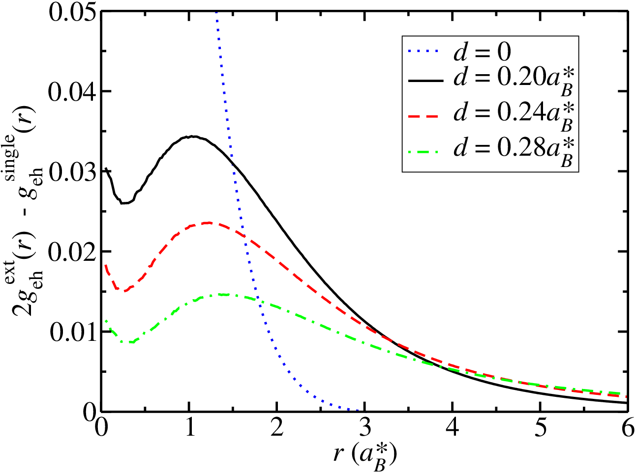
Figure 8 shows the electron-hole PDF for a single exciton, , obtained from the exact numerical solution to Eq. (2) in Ref. 7. Figures 9 and 10 show electron-electron and electron-hole PDF’s, respectively, for the biexciton system with . At smaller layer separations the electron-hole PDF exhibits a larger peak at zero interparticle separation, and decays more rapidly with interparticle distance.
The size of the biexciton is most easily judged by examining the electron-electron PDF (which is identical to the hole-hole PDF for ). The size of the biexciton diverges as the critical layer separation ( for ) is approached. At zero layer separation, the electron-electron PDF is negligible for interparticle distances larger than and has a maximum at .
Although a second peak cannot be discerned in Fig. 10, the quantity plotted in Fig. 11 allows one to see the inter-exciton electron-hole PDF superimposed on the change in the intra-exciton PDF due to the presence of the other exciton. The peaks in Fig. 11 occur at the same separation as those in Fig. 9, confirming that excitons retain their identity in bound biexcitons for large layer separations, even when electrons and holes have equal masses. For zero layer separation there is no discernable peak, however, and the function rises sharply to a maximum at zero interparticle separation. This may be due to the large change in the single-exciton PDF due to the presence of the other exciton swamping the inter-exciton electron-hole PDF. We are thus unable to conclude with certainty that excitons retain their identities in bound biexcitons throughout the region of biexciton stability.
V Conclusions
We have carried out a QMC study of the interaction between pairs of excitons in bilayer systems. We have calculated the exciton-exciton interaction potential by constraining the center-of-mass separation, which we believe gives a more accurate pair potential at short range than the potential calculated by assuming the holes to be infinitely heavy.[8] We find that for large layer separations, excitons retain their identity when they bind to form a biexciton, suggesting that treating excitons as individual particles is a reasonable approximation. However, by solving the Schrödinger equation for all four particles in a biexciton, we find that the range of layer separations and mass ratios over which biexcitons are stable is somewhat larger than the region of stability predicted using exciton-exciton pair potentials.
VI Acknowledgments
Financial support has been provided by the UK Engineering and Physical Sciences Research Council and Jesus College, Cambridge. Computing resources have been provided by the Cambridge High Performance Computing Service. We would like to thank C. Schindler for providing the data shown in Figs. 1, 2, 3, and 4. We thank P. López Ríos for assistance with the calculations.
Appendix A Fit to the exciton-exciton potential
| Parameter | |||
|---|---|---|---|
The exciton-exciton potential curves with in Fig. 6 may be fitted to a function of the form,
| (7) | |||||
where is the layer separation and are the fitting parameters. The function has the correct long-range behavior, for . The fitting parameter values are shown in Table 1.
The interaction potentials in Fig. 5 with may be fitted to a function similar to Eq. (7). This time the form is
| (8) |
| Parameter | |||
|---|---|---|---|
where the long range behavior is once again reproduced correctly and each of the terms in the first bracket has a physical interpretation. The term may be associated with quadrupole-quadrupole repulsion and the term with van der Waals attraction. The signs of the fitting parameters are consistent with this interpretation for and . The parameter values are shown in Table 2.
References
- [1] D. W. Snoke, Science 298, 1368 (2002).
- [2] L. V. Butov, A. C. Gossard, and D. S. Chemla, Nature 418, 751 (2002).
- [3] L. V. Butov, J. Phys.: Condens. Matter 16, R1577 (2004).
- [4] R. Rapaport, G. Chen, D. Snoke, S. H. Simon, L. Pfeiffer, K. West, Y. Liu, and S. Denev, Phys. Rev. Lett. 92, 117405 (2004).
- [5] A. T. Hammack, M. Griswold, L. V. Butov, L. E. Smallwood, A. L. Ivanov, and A. C. Gossard, Phys. Rev. Lett. 96, 227402 (2006).
- [6] M. H. Szymanska and P. B. Littlewood, Phys. Rev. B 67, 193305 (2003).
- [7] M. Y. J. Tan, N. D. Drummond, and R. J. Needs, Phys. Rev. B 71, 033303 (2005).
- [8] C. Schindler and R. Zimmermann, Phys. Rev. B 78, 045313 (2008).
- [9] L. V. Butov, Solid State Commun. 127, 89 (2003).
- [10] D. W. Snoke, Phys. Stat. Sol. (b) 238, 389 (2003).
- [11] R. Zimmermann and C. Schindler, Solid State Commun. 144, 395 (2007).
- [12] W. M. C. Foulkes, L. Mitas, R. J. Needs, and G. Rajagopal, Rev. Mod. Phys. 73, 33 (2001).
- [13] D. M. Ceperley and B. J. Alder, Phys. Rev. Lett. 45, 566 (1980).
- [14] N. D. Drummond, M. D. Towler, and R. J. Needs, Phys. Rev. B 70, 235119 (2004).
- [15] T. Kato, Commun. Pure Appl. Math. 10, 151 (1957); R. T. Pack and W. B. Brown, J. Chem. Phys. 45, 556 (1966).
- [16] R. J. Needs, M. D. Towler, N. D. Drummond, and P. López Ríos, CASINO version 2.2 User Manual, University of Cambridge, Cambridge (2008).
- [17] C. J. Umrigar, K. G. Wilson, and J. W. Wilkins, Phys. Rev. Lett. 60, 1719 (1988).
- [18] P. R. C. Kent, R. J. Needs, and G. Rajagopal, Phys. Rev. B 59, 12344 (1999).
- [19] N. D. Drummond and R. J. Needs, Phys. Rev. B 72, 085124 (2005).
- [20] C. J. Umrigar, J. Toulouse, C. Filippi, S. Sorella, and R. G. Hennig, Phys. Rev. Lett. 98, 110201 (2007).
- [21] A. D. Meyertholen and M. M. Fogler, arXiv:0808.2067v1 [cond-mat.mes-hall]
- [22] J. Usukura, Y. Suzuki, and K. Varga, Phys. Rev. B 59, 5652 (1999).