,
Can a matter-dominated model with constant bulk viscosity drive the accelerated expansion of the universe?
Abstract
We test a cosmological model which the only component is a pressureless fluid with a constant bulk viscosity as an explanation for the present accelerated expansion of the universe. We classify all the possible scenarios for the universe predicted by the model according to their past, present and future evolution and we test its viability performing a Bayesian statistical analysis using the SCP “Union” data set (307 SNe Ia), imposing the second law of thermodynamics on the dimensionless constant bulk viscous coefficient and comparing the predicted age of the universe by the model with the constraints coming from the oldest globular clusters.
The best estimated values found for and the Hubble constant are: and with a (). The age of the universe is found to be Gyr. We see that the estimated value of as well as of are very similar to those obtained from CDM model using the same SNe Ia data set. The estimated age of the universe is in agreement with the constraints coming from the oldest globular clusters. Moreover, the estimated value of is positive in agreement with the second law of thermodynamics (SLT).
On the other hand, we perform different forms of marginalization over the parameter in order to study the sensibility of the results to the way how is marginalized. We found that it is almost negligible the dependence between the best estimated values of the free parameters of this model and the way how is marginalized in the present work.
Therefore, this simple model might be a viable candidate to explain the present acceleration in the expansion of the universe.
pacs
95.36.+x, 98.80.-k, 98.80.Es1 Introduction.
In the last ten years the observations of type Ia supernovae (SNe Ia) have suggested a possible late time accelerated expansion of the universe (see for instance [1]-[7] and references therein). This discovery has additional support from the cosmic microwave background [8] and the large scale structure [9] observations.
Several models have been proposed to explain this recent acceleration, one of them is the assumption of the existence of the so-called dark energy as responsible of such acceleration, i.e., a new unknown component that must be of the total content of matter and energy in the universe [1]-[7]. The leading dark energy candidates are a cosmological constant and a slowly varying rolling scalar field (quintessence models) [10]-[14]. However, a cosmological constant model faces several strong problems, one of them is the huge discrepancy between its predicted and observed value (of about 120 orders of magnitude) [15]-[18], another one is the so-called the “cosmic coincidence problem”, i.e., why are we living in a moment where the matter density in the universe is of the same order than the dark energy density? [19]-[21].
On the other hand, it has been known since several years ago before of the discovery of the present acceleration in the expansion of the universe that a bulk viscous fluid can produce an accelerating cosmology (although it was originally proposed in the context of an inflationary period in the early universe) without the need of any cosmological constant or dark energy component [22]-[35] although some authors do not agree with this conclusion [36].
So, it is natural to think of the bulk viscous pressure as one of the possible mechanism that can accelerate the universe today (see for instance [37]-[46], where in some of these works the bulk viscous coefficient is assumed a priori without being derived from known physics or known particle properties). However, this idea faces the problem of that it is necessary to propose a viable mechanism for the origin of the bulk viscosity and in this sense some proposals have been already suggested [47]-[50].
Nowadays, with the observational data sets of SNe Ia [1]-[7] and some other cosmological observations like the shift parameter of the cosmic microwave background radiation (CMB) given by the Wilkinson Microwave Anisotropy Probe (WMAP) observations [51], and the baryon acoustic oscillation (BAO) measurement from the Sloan Digital Sky Survey (SDSS) [52] it is possible to test cosmological models. So, in the present work we study and test bulk viscous matter-dominated cosmologies, i.e., scenarios which the only component of the universe is a pressureless fluid with bulk viscosity. The pressureless fluid characterizes to both baryon and dark matter components. The idea of this model is to explain the present acceleration of the universe using the bulk viscous pressure of the fluid without the need of any dark energy.
As it was mentioned above, the explicit form of the bulk viscosity has to be assumed a priori or obtained from a known physical mechanism. In the present work we choose the first possibility. So, we assume a constant bulk viscous coefficient that it is the simplest parametrization for the bulk viscosity and we estimate its value using SNe Ia observations. The theoretical solution of this model has been also analyzed in [22], [53]-[56] and other parametrizations for the bulk viscous coefficient have been also proposed and studied in [37]-[45] and [57]-[60]. There is also other general approach to the bulk viscous cosmologies called “fluids with inhomogeneous equation of state” (see [61, 65]).
In section 2 we present the generalities of bulk viscous fluids in General Relativity (GR), in section 3 we apply this formalism to a bulk viscous matter-dominated universe model where we find the explicit expression for the Hubble parameter in function of the redshift. In section 4 we analyze the behavior of the scale factor for the possible scenarios that the model predicts for the universe according to the value of the bulk viscous coefficient. In section 5 we study the behavior of the deceleration parameter , the curvature scalar , the total matter density and the age of the universe and in section 6 we briefly review the second law of thermodynamics (SLT). Section 7 presents the SNe Ia test to constrain the model and compute the best estimated values for the bulk viscous coefficient and the Hubble constant. After that, section 8 presents the best estimated values and the probability distribution functions for the bulk viscous coefficient by marginalizing over the Hubble constant assuming three different priors and finally in section 9 we present our conclusions. The appendices A, B and C detail the marginalization methods used in the present work.
2 Theory of relativistic bulk viscous fluids.
The origin of the bulk viscosity in a physical system is due to its deviations from the local thermodynamic equilibrium (for a review in the theory of relativistic dissipative fluids see [66]). In a cosmological fluid, the bulk viscosity arises when the fluid expands (or contracts) too fast so that the system does not have enough time to restore the local thermodynamic equilibrium and then it appears an effective pressure restoring the system to its local thermodynamic equilibrium. The bulk viscosity can be seen as a measurement of this effective pressure. When the fluid reaches again the thermal equilibrium then the bulk viscosity pressure ceases [49], [67]–[69].
In an accelerated expanding universe it is very possible that the expansion process is actually a collection of states out of thermal equilibrium in a small fraction of time. So, it is natural to assume the existence of a bulk viscous coefficient in a more realistic description of the accelerated universe today.
We use the Weinberg formalism [70]–[72] for the imperfect fluids. So, in the present work we consider a bulk viscous fluid as source of matter in the Einstein fields equations , where is the Newton gravitational constant.
On the other hand, the energy-momentum tensor of an imperfect fluid with a first-order deviation from the thermodynamic equilibrium has the form [49, 70, 71]:
| (1) |
where
| (2) |
In the equations (1) and (2) the four-velocity vector is of an observer who measures the effective pressure , and are the pressure and density of the fluid respectively. The term is the bulk viscous coefficient that arises in the fluid which is out of the local thermodynamic equilibrium.
It can be seen that the energy-momentum tensor (1) is similar to that of a perfect fluid but with an effective pressure composed by the usual pressure of the fluid plus the pressure due to its bulk viscosity . This viscous pressure, , can be seen as a “measurement” of the pressure to restore the local thermodynamic equilibrium [49], [67]–[69]. The conservation equation for the viscous fluid is
| (3) |
The effective pressure (2) was originally proposed by Eckart [74] in 1940 for a relativistic dissipative process in the context of thermodynamics systems out of local equilibrium, and subsequently Landau & Lifshitz presented an equivalent formulation [75].
However, the Eckart theory has problems in several aspects. One of them is that all the equilibrium states in this theory are unstable [76]. Another one is that signals can propagate through the fluids with superluminal velocities [77, 78].
In 1979, Israel-Stewart [79, 80] developed a more consistent and general theory that avoids these problems, and from which the Eckart theory is the first-order limit of the Israel-Stewart theory when the relaxation time goes to zero. Nevertheless, the Eckart theory is simpler to deal with than the Israel-Stewart theory.
Despite of the inherent problems of the Eckart theory, and due to that it is simpler than the Israel-Stewart theory, it has been widely used recently by several authors to model bulk viscous dark fluids as responsible of the recent observed acceleration of the universe assuming that the approximation is valid for this purpose (see, for instance [37]-[41], [44, 45, 49, 56, 60]), i.e., in these papers assume a vanishing relaxation time, so that, in this limit the Eckart theory is a good approximation to the Israel-Stewart theory. In this context, it is convenient to mention that Hiscock et al[36] showed that flat Friedmann-Robertson-Walker cosmological models containing a bulk viscous Boltzmann gas expand more rapidly using the Eckart theory than the Israel-Stewart one, and suggesting that inflationary acceleration driven by bulk viscosity could be an effect of applying a pathological theory such as the Eckart theory. These results suggest that in this context the use of the Israel-Stewart causal theory would not produce a recent accelerating epoch as the Eckart theory would. However, posterior studies have suggested that this conclusion could not be true because consistent inflationary solutions have been found using the Israel-Stewart theory [34, 35].
It is important to point out that there exists other more general formulation for irreversible processes than the Israel-Stewart theory developed by D. Pavón et al. where the temperature is not necessary that of the thermodynamic equilibrium, see [81] for details. In the present work we assume the Eckart theory and we constrain the model described above using SNe Ia observations.
3 Cosmological model of bulk viscous matter-dominated universes.
We study a cosmological model in a flat universe where the only component is a pressureless fluid with constant bulk viscosity as an explanation for the present accelerated expansion of the universe. The pressureless fluid characterizes both the baryon and dark matter components.
Note that this model does not have the Cosmic Coincidence problem and that this fluid represents an unified description of the dark sector plus the baryon component in a similar way than the Chaplygin gas model (see for instance [44, 82] and references therein). In this approach the present acceleration of the universe is driven by the bulk viscous pressure of the fluid instead of a dark energy component. The present work differs from the approach of Colistete et al[44] in that they propose two fluids, one of them is a bulk viscous fluid representing in an unified way the dark sector with a bulk viscous coefficient proportional to a power of the energy density (i.e., , with constants), and the other one is a pressureless fluid representing the baryon component. Nevertheless, most of their analysis and test using cosmological observations is done using the ansatz .
Since we work with a pressureless fluid () then , where is the bulk viscous coefficient of the matter fluid.
We consider a spatially flat geometry for the Friedmann-Robertson-Walker (FRW) cosmology as favored by WMAP [83]
| (4) |
where the function is the scale factor. On the other hand, we spread the conservation equation (3) in all its components
| (5) |
where is the Hubble parameter, is the total matter density, the dot means time derivative and .
The conservation equation (5) can be written in terms of the scale factor as
| (6) |
This equation is valid for any parametrization of , in particular we assume the ansatz constant that it is perhaps the simplest parametrization for the bulk viscous coefficient that can be proposed. Its value is going to be estimated from the SNe Ia observations.
On the other hand, the first Friedmann equation for a flat universe is
| (7) |
So, substituting (7) into (6) we obtain
| (8) |
Changing of variable from the scale factor to the redshift using the relationship11 1 We assume that the value of the scale factor evaluated today is equal to one. , we obtain the ordinary differential equation (ODE):
| (9) |
The exact solution of this ODE is:
| (10) |
where is the matter density evaluated today. Substituting this solution into (7) we obtain
| (11) |
where is the Hubble constant and where we have defined the dimensionless bulk viscous coefficient , the matter density parameter and the critical density today as:
| (12) |
4 Classification and evolution of bulk viscous matter-dominated models.
In this section we classify all the possibilities for the universe predicted by this bulk viscous matter-dominated model using different values of the constant bulk viscous coefficient. Note that we have one different model for each value of , so actually we have a collection of models depending of the value of .
We analyze the theoretical behavior of the scale factor in terms of the cosmic time. We begin expressing (13) in terms of the scale factor
| (14) |
Integrating (14) yields
| (15) |
where labels the cosmic time and the cosmic time today.
4.1 Case .
When we recover the usual matter-dominated universe (with null bulk viscosity) with a scale factor coming from the integration of (15) like:
| (16) |
The first and second derivatives of the scale factor with respect to are
| (17) |
and
| (18) |
This case predicts an eternal decelerated expanding universe (see figures 1–7). In this case the curvature scalar and the matter density are and respectively, that both diverge when the scale factor goes to zero (see sections 5.2 and 5.3 for details). When we have these two conditions ( and ) in the past of the universe we say that there was a Big-Bang. The elapsed time between the Big-Bang time till today is
| (19) |
where the subscript ‘B’ stands for “Big-Bang”. On the other hand, when then and decrease to zero.
4.2 Case .
For we do the change of variable in expression (15) yielding:
| (20) |
This last expression can be rewritten as
| (21) |
When we can remove the absolute value bar of the right hand side term and then we obtain
| (22) |
The first and second derivative of the scale factor with respect to are
The case does not correspond to a physical case of our interest because this case predicts an eternal contraction of the universe ( for any value of the cosmic time ) that is in contradiction with the observations (see the expression (14) to note that implies ).
In order to study carefully the expression (22) for different values of we take four cases:
- •
- •
- •
- •
4.2.1 Case .
From the expression (22) we can see that when then the scale factor tends to have the form like that of the de Sitter universe, i.e.,
| (25) |
On the other hand, for any value of in this interval all the models predict an universe having a Big-Bang in the past in the cosmic time:
| (26) |
So, the universe begins with a Big-Bang followed by an eternal expansion (there is not any recollapse epoch, see figures 1 and 2) and this expansion begins with a decelerated epoch followed by an eternal accelerated one (see figures 2 and 3).
The transition between the decelerated–accelerated expansion epochs depends on the value of . We compute the value of the scale factor where the transition happens. For that, we derive to with respect to using the expression (14):
| (27) |
Then, we make equal to zero to expression (27) in order to obtain the value of the scale factor “” where the transition happens, obtaining
| (28) |
where the subscript “t” stands for “transition”. Writing the expression (28) in terms of the redshift yields
| (29) |
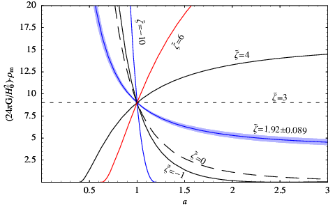
From the expression (28) we can see that for values of in the interval the transition between the decelerated epoch to the accelerated one takes place in the future (). When , the value of tends to infinity in the future. When then the transition takes place today (), when the transition takes place in the past of the universe () and when the value of is closer to 3, the transition is closer to the Big-Bang time (see figures 2–4 and 7).


The curvature scalar is always positive and it has a very large value when the scale factor is very small (at the Big-Bang time) and it decreases forever tending to its minimum value when (see section 5.2 and figure 8) what is the de Sitter universe (consistent with the expression (25)). In the same way, the matter density is also very large when the scale factor is very small (at the Big-Bang time) and it decreases forever tending to its minimum value when (see section 5.3).
The possible value for at least at the 99.9% confidence level estimated from the SCP “Union” SNe Ia data set is in the interval . So, assuming the best estimated value (see table 1), the value of the scale factor at the transition time between deceleration–acceleration epochs is (see expression (28)): (. Note that the transition comes directly from the model, it is not necessary to assume any particular ansatz to estimate or induce it.
4.2.2 Case .
In the expression (22) we put to obtain
| (30) |
This case corresponds to the de Sitter universe. Figures 1–5 show the behavior of expression (30) (the short-dashed lines). The scale factor becomes zero just when and when the scale factor increases to infinity.
In this case the model predicts an universe in an eternal accelerated expansion. The curvature scalar and the matter density are constants with values and respectively. See sections 5.2 and 5.3 for details.
Note that this model does not have a Big-Bang because the curvature scalar and the matter density are regular for any value of the cosmic time.
4.2.3 Case .
This case predicts an universe expanding forever, and this expansion is always accelerated (there is not any decelerating epoch or acceleration-deceleration transition).
In this case when then the scale factor tends to the form of the de Sitter universe in the future (see expression (25)) and when then the universe tends to an Einstein static universe (defined by ) where the value of the scale factor is not zero but tends to its minimum value:
| (31) |
and during the evolution of the universe the scale factor is an increasing monotonic function with respect to the cosmic time. Thus, for this case there was not a Big-Bang and the age of the universe is not defined. Figure 5 shows some plots of the expression (22) for different values of .

4.2.4 Case .
This case predicts an eternal decelerated expanding universe. The universe begins with a Big-Bang and expands forever until to reach its maximum value when , becoming an Einstein static universe in the future. The Big-Bang took place in the cosmic time defined by expression (26). Figures 2–4 and 6 show the behavior of the scale factor for this case.
In this case the curvature scalar has a transition from positive to negative values at . When then (the Big-Bang) and when the curvature scalar is zero. The minimum value of the curvature scalar is negative and it is reached at the value of the scale factor . See section 5.2 and figure 8 for details.

5 Cosmological parameters.
5.1 Deceleration parameter .
We study the behavior of the deceleration parameter function that is defined as
| (32) |
The term can be calculated from the second Friedmann equation, that for a matter-dominated universe with bulk viscosity reads:
| (33) |
From the definition of (see expression in (12)) we have that
| (34) |
On the other hand, from the first Friedmann equation (7) we have
| (35) |
So, substituting the expressions (34) and (35) in (33) we obtain:
| (36) |
Thus, substituting (36) in (32) yields
Using equation (14) for we arrive to
| (37) |
Figure 7 shows the behavior of expression (37). Note that this expression does not depend on . We summarize the behavior of the deceleration parameter according to different values of as follows:
- •
When we have that corresponds to a matter-dominated universe with null bulk viscosity.
- •
When we have that corresponds to de Sitter universe.
- •
Case : It is always a decreasing function from to with a transition from positive to negative values in the value of the scale factor (see expression (28)).
- •
Case : When then where is the minimum value of the scale factor (see expression (31)) and when then . It is a negative and increasing function but it never becomes positive, its maximum value is -1.
- •
Case : When then and when then where is the maximum value of the scale factor. It is a positive and increasing monotonic function where its minimum value is .
From the expression (37) we obtain the deceleration parameter evaluated today as
| (38) |
Note that when the transition from the decelerated to accelerated epochs of the universe takes place today. For we have a decelerated universe in the present and for we have an accelerated one today.
Assuming the best estimated values for from table 1, the deceleration parameter today is (see expression (38)): .

5.2 The curvature scalar .
We calculate the curvature scalar in order to study the singularities of the model. For a flat universe it is defined as
| (39) |
| (41) |
- •
When then that corresponds to a matter-dominated universe with null bulk viscosity.
- •
When then that corresponds to de Sitter universe.
- •
Case : When then (the Big-Bang singularity). It is always a positive and decreasing function until to reach its minimum value when .
- •
Case : It is always a positive and increasing function from zero at (where is the minimum value of the scale factor) until to reach its maximum value when .
- •
Case : When then (the Big-Bang singularity). The curvature scalar is zero at the values of the scale factor and , where
(42) and is the maximum value for the scale factor defined in expression (31). At there is a transition from positive to negative values of . When the curvature scalar is a positive and decreasing function. For the value of is negative. The minimum value of the curvature scalar is at the value of the scale factor
(43)

5.3 The matter density .
We calculate the matter density predicted for this model. We substitute the Hubble parameter (expression (14)) into the expression (35) for the matter density, yielding
- •
When then that corresponds to a matter-dominated universe with null bulk viscosity.
- •
When then that corresponds to de Sitter universe.
- •
Case : When then (the Big-Bang singularity). It is a decreasing function until to reach its minimum value when .
- •
- •
Case : When then (the Big-Bang singularity). It is a decreasing function until to reach its minimum value in .
5.4 The age of the universe.
We define the age of the universe as the elapsed time between the Big-Bang time until today . So, from the expression (19) for the case we have
| (45) |
And from the expression (26) for the case
| (46) |
Note that for the case the age of the universe is not defined. On the other hand, evaluating the expression (46) in the best estimated values of and from the SCP “Union” SNe Ia data set (see table 1) yields an age of Gyr. The errors are at 68.3% confidence level. We found that this age is in perfect agreement with the constraints on the age of the universe coming from the oldest globular clusters [85]. Figure 10 shows the age of the universe for different values of and the best estimate, the vertical lines correspond to 22 2 Hereinafter the units of are expressed in , it is the permitted region according to values of consistent with the distance moduli used to derive ages for Galactic globular clusters from the Hipparcos parallaxes. As a reference, the predicted age of the universe for CDM (Lambda Cold Dark Matter) cosmological model with a flat universe and using the best estimated values of and shown in table 1 is Gyr.

6 Thermodynamics and the local entropy.
The law of generation of the local entropy in the FRW space–time is found to be [70, 71, 72]
| (47) |
where is the temperature and is the rate at which entropy is being generated in an unit volume. Then, the second law of the thermodynamics can be written as
| (48) |
which, from the expression (47), it implies that .
Since the Hubble parameter is positive in an expanding universe then has to be positive in order to preserve the validity of the second law of the thermodynamics. Thus, equation (48) can be written for this model as
| (49) |
7 Type Ia Supernovae test.
We analyze and constrain the viability of the model using the type Ia supernovae (SNe Ia) observations and the entropy tests (see expression (49) and section 6). For that, we calculate the best estimated values for the parameters and and the goodness-of-fit of the model to the data by -minimization and then compute the confidence intervals for and the probability density functions for (marginalizing over ) to constrain their possible values.
We perform the statistical analysis using the “Union” SNe Ia data set of “The Supernova Cosmology Project” (SCP) [73] composed by 307 type Ia supernovae brought together from 13 independent data sets.
where is the Hubble parameter (expression (13)) and ‘’ is the speed of light. The theoretical distance moduli for the -th supernova with redshift is defined as
| (51) |
where and are the apparent and absolute magnitudes of the SNe Ia respectively and the superscript ‘t’ stands for theoretical. We construct the statistical function as
| (52) |
where is the observational distance moduli for the -th supernova, is the variance of the measurement and is the amount of supernovae in the data set.
Once constructed the function (52), we numerically minimize it to compute the “best estimates” for the free parameters of the model (i.e., ). The function measures the goodness-of-fit of the model to data. The probability density function (pdf) is defined as
| (53) |
where ‘cte’ is a normalization constant.
So, we minimize the function to obtain the results shown in table 1. The confidence intervals for and are shown in figure 11. Note that at least at the 99.73% confidence level the possible values for are inside of the interval . The models in this interval indicate the existence of a Big-Bang in the past of the universe, they have an accelerated expansion today and predict an age of the universe Gyr at the 99.73 % confidence level (see figure 11 and subsections 4.2.1, 5.4).
In order to compare the results shown in table 1 (in particular the measurement of the goodness-of-fit to data and the best estimated value for ) with other models we compute also the best estimated values for the CDM model using the same SNe Ia data set. For the CDM model, we assume a flat cosmology with and as free parameters (implying that the cosmological constant density parameter is ). The results are shown in Table 1.
We find that the best estimated values for and the goodness-of-fit to data from CDM model are very similar to those obtained from the bulk viscous model using the same SCP “Union” SNe Ia data set and in agreement with that reported by 5 year WMAP ( (km/s)Mp, see [83]).

| Viscous model constant | |||||
|---|---|---|---|---|---|
| Model | |||||
| Constant bulk viscosity | 1 | 314.57 | 1.031 | ||
| CDM | — | 311.84 | 1.022 | ||
8 Marginalization over
Now, we construct a pdf for the bulk viscous coefficient marginalizing over the Hubble constant in order to have to as the only free parameter of the model. We use three different priors to marginalize :
| Viscous model constant | |||
|---|---|---|---|
| Best estimates for | |||
| Marg. | |||
| (i) | 331.30 | 1.08 | |
| (ii) | 315.26 | 1.03 | |
| (iii) | 314.91 | 1.02 | |
| (iv) | 316.75 | 1.03 | |
| (v) | 330.41 | 1.07 | |
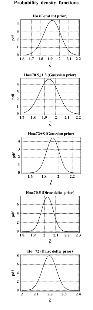
8.1 Marginalization assuming a constant prior over .
8.2 Marginalization assuming a Gaussian prior over .
We marginalize over by assuming a Gaussian prior as described in B. We use two different central values for the Gaussian prior for , they are and as suggested by 5 year WMAP data [83] and HST Cepheid variable star observations [89] respectively. See section B for details. The results are shown in table 2 and figure 12.
8.3 Marginalization assuming a Dirac delta prior over .
Finally, we marginalize over by assuming a Dirac delta prior as described in C. In practice, it means to assume a specific value for . In the same way as above we use two different values for , they are and . The results are shown in table 2 and figure 12.
9 Conclusions.
We performed a detailed study of a bulk viscous matter-dominated universe model with constant bulk viscous coefficient . The only component of this model is a pressureless fluid with an assumed constant bulk viscosity driving the present accelerated expansion of the universe. We analyzed the different possible scenarios for the behavior and evolution of the universe predicted by the model according to the value of the dimensionless bulk viscous coefficient . In general, the model predicts an expanding universe for any value of and we find that for values of in the range the model predicts an universe with a Big-Bang in the past and then starting with a decelerated expansion epoch followed by a transition to an accelerated epoch in late times.
The case corresponds to the de Sitter universe. When the universe is always in an accelerated expansion and the value of the scale factor tends to infinity in the future (in a similar way than the de Sitter universe) and where the curvature scalar goes to a positive constant value. In this case there is not a Big-Bang nor a defined age nor origin of the universe because the scale factor has a minimum value greater than zero in the past of the universe (when ), where also, the curvature scalar and the matter density are zero, i.e., we have the Einstein static universe in the past.
When the universe is always in a decelerated expansion and the scale factor tends to a finite value in the future (it tends to the Einstein static universe in the future) where also, the curvature scalar and the matter density go to zero. For in this range there is always a Big-Bang in the past.
For any value of there does not exist any recollapse epoch or transition between expansion to contraction epochs. When the transition between a decelerated to accelerated epoch takes place today (i.e., for ). For the transition between the deceleration–acceleration epoch takes place in the future and for the transition took place in the past.
On the other hand, we estimate the values of and using the SCP Union SNe Ia data set where it is found that the estimated values of are positives, in agreement with the second law of thermodynamics. We note that the best estimated value for is in agreement with that reported by 5 year WMAP and estimated from CDM model (using the same SNe Ia data set) and the minimum value of the function () obtained is of the same order than that obtained for CDM model indicating that this is a competitive model to fit the supernova observations.
We estimate and compare the age of the universe predicted by this model with the constraints on the age coming from the oldest globular cluster observations. We find that the best estimated values for the age of the universe is Gyr that is in agreement with the constraint in the age coming from the oldest globular clusters.
The present model has been constrained using SNe Ia data. It means that we have constrained the model using information (observations) of the past of the universe until a redshift . So, SNe Ia observations are not enough to trace the whole evolution of the universe from the Big-Bang until the present time. Therefore, it would be important to constrain the model using also cosmological observations that can provide information of the early universe like the observations of the CMB anisotropies from the WMAP experiment and the large scale structure (LSS) from SDSS experiment. A preliminary work in that sense has been already done in [56] showing (but not in a conclusive way) that when the model is constrained using the shift parameter of CMB and the parameter measuring the BAO peak from SDSS, in addition to the Gold 2006 SNe Ia data set, the estimated value of is negative at 99.7% confidence level, violating the second law of thermodynamics and the estimated value of is lower () than that reported by 5 year WMAP and HST Cepheid variable star observations and giving a bad goodness-of-fit to data. Considering these facts we may conjecture that this model does not work well for early times of the universe and that in order to be a viable model the bulk viscosity should be triggered just until late times.
Another problem of the model is to explain the origin of the bulk viscosity from known or new physics. Some proposals in that sense have been explored, for instance in [49] and [50], where it is proposed a mechanism to generate the bulk viscosity by the decay of dark matter particles into relativistic products.
Finally, we explore also the sensitivity of the results to different ways of marginalization over when we estimate just the coefficient . We find that it is almost negligible the difference in the estimations of when is marginalized assuming constant and Gaussian priors centered in the values reported by 5 year WMAP and HST Cepheid variable star observations. However, when is marginalized by assuming a specific value (a Dirac delta prior located at the values reported as mentioned above) the estimated values of have a small increase and the values of increase as well (i.e., we have a worse fit to data).
10 Acknowledgements.
We thank Jose Antonio González for his comments on the constraints for the age of the universe, Francisco S. Guzmán and Olivier Sarbach for useful discussions during the preparation of this work. We also thank John Barrow for his useful comments on previous works done on this topic. We acknowledge to the Instituto Avanzado de Cosmología (IAC) for its partial support and useful seminars. This work was in part supported by grants SNI-20733, CIC-UMSNH No. 4.8, UMSNH-CA-22 and COECyT–FIFOECYT 2008.
Appendix A Marginalization assuming a constant prior over .
To construct a pdf that depends only on the parameter we use the process of marginalization over in order to eliminate the dependence of the pdf with respect to the parameter .
The following procedure can be applied for any other model. It is, in a model with several parameters where it is necessary to reduce the number of free parameters or, for some reason, to eliminate the dependance of the model from some particular free parameters (for instance: ) in order to compute the best estimated values of the other free parameters that we keep (in our case: ) the solution is to marginalize over the parameters that we want to eliminate.
In the present work we assume three different prior distribution functions for : constant, Gaussian and Dirac delta. In this appendix we describe the marginalization using a constant prior for .
We start by multiplying and dividing by the equation (50)
| (54) |
Next, we define a new dimensionless luminosity distance as . Then
| (55) |
where does not depend on anymore and .
The theoretical distance moduli (51) becomes
| (56) |
where we have defined a dimensionless “Hubble parameter” . It is useful to define a new theoretical distance moduli that does not depend on anymore as
| (57) |
Then, the expression (56) for the distance moduli becomes
| (58) |
Now we construct the function (52) with these new definitions as
| (59) |
where is the observed distance moduli and its variance.
We rewrite the expression (59) as
| (60) | |||||
If we define 33 3 Note that these expressions do not depend on anymore.
| (61) |
then we can express (60) as
| (62) |
where
| (63) |
Note that all the dependence of the function with respect to is now in the variable. Remind that the pdf is defined as
| (64) |
where “cte” is a normalization constant. So, we marginalize the pdf (64) over computing the following integration
| (65) |
where is the prior probability density function for . In general, the integration (65) has to be done over the range of all the possible values of the parameter to be marginalized. In this case the range of possible values for , or equivalently , is .
If we take the case where the prior for is a constant then:
| (66) |
A constant prior means that we do not prefer any particular value for , i.e., any value for has the same probability of being. To solve the integral (66) we do a change of variable from to (see expression (63)). At the same time, we substitute the expression (62) into (64) and then (64) into (66), yielding
| (67) |
where .
We can see that the integral (67) has the form of a Gaussian distribution with value:
| (68) |
where is the mean and is the variance of the distribution.
Therefore the expression (67) becomes
| (69) |
so that the does not depend on anymore. Note that it was not necessary any numerical integration of the expression (66). We can express this in terms of a new function like
| (70) |
where and
| (71) |
This new function does not depend on anymore. The label “cp” stands for constant prior for .
Appendix B Marginalization assuming a Gaussian prior over .
We perform the marginalization assuming a Gaussian probability distribution function for centered at and with standard deviation . So, the pdf () prior with the form of a Gaussian distribution for is
| (72) |
With this, the expression (65) becomes
| (73) |
where the function is given by (62) and “cte” is a normalization constant.
In the present work we use two different central values for the Gaussian prior coming from two different observations. One of them, is that coming from the 5 year WMAP observations where with an standard deviation of . The other central value is with an standard deviation of as reported by the HST Cepheid variable star observations.
In practice we perform the numerical integration of the expression (73) in the interval considering that this is a suitable and representative interval that include almost the 100% of the probability density for .
Appendix C Marginalization assuming a Dirac delta prior over .
It means to assume a specific value of . It is like to think that the value of the Hubble constant is that has been measured with an infinite accuracy (with standard deviation equal to zero), so that its pdf() has the form of a Dirac delta function.
Clearly, this assumption is just an idealization to simplify the work and it does not correspond to the reality. However, for some cases it is a good approximation. This prior has the advantage of that once assumed it is very simple to perform the integration of the expression (65) using the Dirac delta properties. Thus, the prior with the form of a Dirac delta for is
| (74) |
With this, the expression (65) becomes
| (75) |
where “cte” is a normalization constant.
References.
References
- [1] Riess A G et al, 1998 Astron. J. 116 1009–1038
- [2] Perlmutter S et al, 1999 Astrophys. J. 517 565
- [3] Riess A G et al, 2004 Astrophy. J. 607, 665–687
- [4] Astier P et al, 2006 Astronomy and Astrophysics 447 31–48
- [5] Riess A G et al, 2007 Astrophy. J. 659 98–121
- [6] Davis et al. 2007 Astrophys. J. 666 716–725.
- [7] Wood-Vasey et al, 2007 Astrophys. J. 666 694–715
- [8] Bennett C L et al, 2003 Astrophys. J. 148 1
- [9] Tegmark M et al, 2004 Phys. Rev. D. 69 103501
- [10] Caldwell R R, Dave R and Steinhardt P J 1998 Appl. Space Sci. 261 303
- [11] Zlatev I, Wang L and Steinhardt P J 1999 Phys. Rev. Lett. 82 896
- [12] Wang L, Caldwell R R, Ostriker J P and Steinhardt P J 2000 Astrophys. J. 530 17
- [13] Steinhardt P J 2003 Phil. Trans. R. Soc. A 361 2497
- [14] Peebles P J E 2003 Rev. Mod. Phys. 75 559–606
- [15] Weinberg S 1989 Rev. Mod. Phys. 61 1
- [16] Carroll S M, Press W H and Turner E L 1992 Annu. Rev. Astron. Astrophys. 30 499–542
- [17] Carroll S M 2001 Living Reviews in Relativity 4 1
- [18] Padmanabhan T 2003 Physics Reports 380, issues 5–6, 235–320
- [19] Steinhardt P J 1997 Critical Problems in Physics, edited by Fitch V L and Marlow D R (Princeton University Press, Princeton, NJ)
- [20] Zlatev I, Wang L and Steinhardt P J 1999 Phys. Rev. Lett. 82 896
- [21] Steinhardt P J, Wang L and Zlatev I 1999 Phys. Rev. D 59 123504
- [22] Heller M, Klimek Z and Suszycki L 1973 Astrophy. and Space Science 20 205–212
- [23] Heller M and Klimek Z 1975 Astrophys. and Space Science 33 L37-L39
- [24] Diosi L, Keszthelyi B, Lukács and Paál G 1984 Acta Phys. Pol. B 15 909; 1985 Phys. Lett. B 157 23
- [25] Morikawa M and Sasaki M 1985 Phys. Lett. B 165 59
- [26] Waga I, Falcao R C and Chanda R 1986 Phys. Rev. D 33 1839
- [27] Barrow J 1986 Phys. Lett. B 180 335
- [28] Padmanabhan T and Chitre S M 1987 Phys. Lett. A 120 443
- [29] Gron O 1990 Astrophys. and Space Science 173 191G
- [30] Beesham A 1993 Physical Rev. D 48 3539
- [31] Diego Pavon and Winfried Zimdahl 1993 Phys. Lett. A 179 261–265
- [32] Maartens R 1995 Class. Quantum Grav. 12 1455–1465
- [33] Coley A A, van den Hoogen R J and Maartens R 1996 Phys. Rev. D 54 1393–1397
- [34] Zimdahl W 1996 Physical Rev. D 53 5483
- [35] Maartens R and Méndez V 1997 Physical Rev. D 55 1937
- [36] Hiscock W A and Salmonson J 1991 Physical Rev. D 43 3249
- [37] Kremer G M and Devecchi F P 2003 Physical Rev. D 67 047301
- [38] Fabris J C Goncalves S V B and de Sá Ribeiro R 2006 Gen. Relativ. Gravit. 38(3), 495–506
- [39] Ming-Guang Hu and Xin-He Meng 2006 Phys. Letters B 635 186–194
- [40] Jie Ren and Xin-He Meng 2006 Phys. Lett. B 633 1–8
- [41] Jie Ren and Xin-He Meng 2006 Phys. Lett. B 636 5–12
- [42] Marek Szydlowski and Orest Hrycyna 2007 Annals Phys 322 2745–2775
- [43] Debnath P S, Paul B C and Beesham A 2007 Phys. Rev. D 76 123505
- [44] Colistete R Jr, Fabris J C, Tossa J and Zimdahl W 2007 Phys. Rev. D 76, 103516, 1–13
- [45] Singh C P, Kumar S and Pradhan A 2007 Class. Quantum Grav. 24 455–474
- [46] Meng X M and Dou X 2008 [arXiv:0812.4904]
- [47] Zimdahl W 2000 Phys. Rev. D 61 083511
- [48] Zimdahl W, Schwarz D, Balakin A B and Pavón D 2001 Phys. Rev. D 64 063501
- [49] Wilson J R, Mathews G J and Fuller G M 2007 Physical Rev. D. 75 043521
- [50] Mathews G J, Lan N Q and Kolda C 2008 Phys. Rew. D 78, 043525
- [51] Wang Y and Mukherjee P 2006 Astrophy. J. 650 1
- [52] Eisenstein D J et al, 2005 (SDSS Collaboration) Astrophy. J. 633, 560–574
- [53] Klimek Z 1974 Acta Cosmologica 2 49
- [54] Heller M and Suszycki L 1974 Acta Phys. Pol B5 345
- [55] Klimek Z 1975 Acta Cosmologica 3 49
- [56] Avelino A, Nucamendi U and Guzmán F S 2008 AIP Conf. Proc. 1026, 300–302. Proc. of the XI Mexican Workshop on Particles and Fields, Tuxtla Gutiérrez, México, nov 7-12, 2007. [arXiv:0801.1686]
- [57] John D Barrow 1987 Phys. Lett. B 180 335–339
- [58] John D Barrow 1988 Nucl. Phys. B 310 743–763
- [59] John D Barrow 1990 String-driven Inflation. In The formation and evolution of cosmic strings eds. G Gibbons & T Vasasparti 449–464 CUP Cambridge.
- [60] Avelino A, Nucamendi 2008 AIP Conf. Proc. 1083, 1–4. Proc. of the III International Meeting on Gravitation and Cosmology, Morelia, México, May 26-30, 2008. [arXiv:0810.0303]
- [61] Nojiri S and Odintsov S D 2005 Phys. Rev. D 72:023003
- [62] Capozziello S et al, 2006 Phys. Rev. D 73:043512
- [63] Mubasher Jamil and Muneer Ahmad Rashid 2008 Eur. Phys. J. C 56 429–434
- [64] Hrvoje Stefancic 2008 [arXiv:0811.4548]
- [65] Hrvoje Stefancic 2008 [arXiv:0812.3796]
- [66] Maartens R 1996 in Proceedings of Hanno Rund Workshop on Relativity and Thermodynamics, South Africa, June 1996 (unpublished) [arXiv:9609119]
- [67] Okumura H and Yonezawa F 2003 Physica A 321 207
- [68] Ilg P and Ottinger H C 1999 Phys. Rev. D 61 023510
- [69] Xinzhong C and Spiegel E A 2001 Mon. Not. R, Astron. Soc. 323 865
- [70] Weinberg S 1972 Gravitation and Cosmology: Principles and Applications of the General Theory of Relativity (John Wiley & Sons, Inc., New York); 1971 Astrophys. J. 168, 175.
- [71] Misner C W, Thorne K S and Wheeler J A 1973 Gravitation (W. H. Freeman and Company) p 567
- [72] Hofmann S, Schwarz D J and Stoecker H 2001 Phys. Rev. D 64 083507
- [73] Kowalski M et al (The Supernova Cosmology Project) 2008 Astrophys. J. 686 749–778
- [74] Eckart C 1940 Physical Rev. 58 919–924
- [75] Landau L D and Lifshift E M 1958 Fluid Mechanics Reading, MA: Addison-Wesley
- [76] Hiscock W A and Lindblom L 1985 Phys. Rev. D 31 725; 1987 Phys. Rev. D 35 3723
- [77] Muller I 1967 Z. Physik 198 329
- [78] Israel W 1976 Ann. Phys., NY 100 310
- [79] Israel W and Stewart J M 1979 Ann. Phys (N.Y.) 118 341
- [80] Israel W and Stewart J M 1979 Proc. R. Soc. A 365 43
- [81] Pavon D, Jou D and Casas-Vázquez J 1982 Ann. Inst. Henri Poincaré Vol. XXXVI 1 79–88
- [82] Mubasher Jamil and Muneer Ahmad Rashid 2008 Eur. Phys. J. C 58 111–114
- [83] Collaboration 5 year WMAP observations 2008 [arXiv:0803.0732]
- [84] Hoyle E 1958. In L’estructure et l’évolution de l’univers Bruxelles, p. 53
- [85] Carreta et al, 2000 Astroph. J. 533 215-235
- [86] Turner M & Riess A G 2002 Astrophy. J. 569, 18
- [87] Sahni V and Starobinsky A A 2000 Int. J. Mod. Phys. D 9, 373; Sahni V 2004 Lect. Notes Phys. 653, 141; Carroll S M 2001 Living Rev. Relativity 4, 1; Padmanabhan T 2003 Phys. Rep. 380, 235; Peebles P J E & Ratra B 2003 Rev. Mod. Phys. 75, 559.
- [88] Copeland E J, Sami M and Tsujikawa S 2006 Int. J. Mod. Phys. D 15, 1753
- [89] Freedman W L et al, 2001 Astrophys. J. 553, 47