Baryon polarization in low-energy unpolarized meson-baryon scattering
Abstract
We compute the polarization of the final-state baryon, in its rest frame, in low-energy meson–baryon scattering with unpolarized initial state, in Unitarized BChPT. Free parameters are determined by fitting total and differential cross-section data (and spin-asymmetry or polarization data if available) for , and scattering. We also compare our results with those of leading-order BChPT.
1 Introduction
The study of spin phenomena in meson–baryon low-energy scattering provides stringent tests of QCD and its associated effective theory, Baryon Chiral Perturbation Theory (BChPT) [1, 2]. Because mesons are spinless, and at low energies can be considered nearly structureless, their scattering off baryons is the simplest process from the point of view of baryon spin dynamics. As such, it is of great interest as a probe of, and may lead to important insights into, the structure and dynamics of baryons.
The applicability of BChPT is limited to the near-threshold energies at which meson momenta are much smaller than the chiral symmetry breaking scale. At moderately higher energies, resonances and coupled-channels effects enter the dynamics that must be either incorporated into the theory or dynamically generated by it. In the three-flavor case those phenomena may be convolved with a strong-coupling regime originating in the large masses of strange hadrons. A well-known example is scattering, in which several strongly-coupled channels are open at threshold, leading to a subthreshold resonance, , and rendering BChPT inapplicable to those processes. Many models and techniques have been developed to overcome those difficulties over a period of several decades, that we cannot review here. In the specific context of BChPT, unitary coupled-channels techniques based on Lippmann–Schwinger or Bethe–Salpeter equations have been succesfully applied to the study of and other meson–baryon processes, even at relatively high energies [3, 4, 5, 6, 7, 8]. A unitarization method dealing directly with the chiral effective theory -matrix has been introduced in [9] in the meson sector, and extended to the baryon sector in [10, 11, 12]. This Unitarized Baryon Chiral Perturbation Theory (UBChPT) has been shown to give accurate descriptions of unpolarized cross-section data in processes [11, 12, 13, 14], and in scattering beyond the resonance peak [10].
In this paper we consider a particular aspect of hadron spin dynamics, the production of polarized baryons in unpolarized meson–baryon scattering. Specifically, we compute the polarization of the final-state baryon in its rest frame in low-energy two-body meson–baryon scattering with unpolarized initial state, in UBChPT. By low energy we mean incident-meson momentum MeV. We use tree-level BChPT partial waves unitarized with the method of [10, 11, 12], and determine their free parameters by fitting total and differential cross-section data (and spin-asymmetry or polarization data if available) for , and scattering. We also compare our results with those of a previous leading-order BChPT calculation [15], with the aim of further probing its domain of applicability.
There is some unavoidable overlap with previous works (e.g., [7, 11, 12]) since we can only fit our calculations to the same available data as used in the previous literature. We remark, however, that although the unitarization method we use is the same as in [11, 12, 16], our approximation scheme is different because we have to include the full - and -channel contributions to scattering and partial waves, as well as baryon decuplet contributions, which are quantitatively important for polarization observables in the energy range considered here. By contrast, in order to obtain a good description of unpolarized cross sections (for, e.g., scattering), it is enough to use less detailed approximations. Good fits to total cross sections can be obtained by considering only -wave scattering, as done at in [11] and at in [14]. 11 1 denotes a generic quantity of chiral order , with a nominally small quantity such as a meson momentum or mass. In [12, 16] unpolarized differential cross sections are described in terms of and partial waves in a non-relativistic approximation in which some of the contributions mentioned above are of subleading order, therefore neglected. This is to be expected, since polarized observables are more sensitive to smaller partial waves than unpolarized ones, the latter being usually dominated by large, resonant waves.
In the following section we present our notation and conventions, give the explicit form of the tree-level partial waves used throughout the paper, and very briefly discuss the unitarization method applied to those partial waves. In sections 3—5 we describe our results for , , and scattering, resp. Detailed fits to scattering data are reported, and the resulting parameters applied to the computation of final-state polarization. In section 6 we give some final remarks.
2 Partial waves and unitarization
The ground-state meson and baryon octets are described by standard [17] traceless complex matrix fields and , resp., with hermitian. We use the physical flavor basis
| (1) |
where are SU(3) Gell-Mann matrices. The real matrices are not hermitian. Their hermitian conjugates form a basis that differs from only in its ordering. To distinguish field components with respect to each of those bases we use lower flavor indices for . Thus, meson and baryon fields are decomposed as22 2 We do not use summation convention for flavor indices. and , with , , and similarly and . Baryon and meson states are denoted and , resp., with the spin along a fixed spatial direction in the fermion rest frame, and , four-momenta. We always use hadron kets with an upper index, and bras with a lower one, with masses and for baryons and mesons resp. Free fields couple to one-particle states as and .
Indices can be raised or lowered by means of the symmetric matrices and . In this basis the structure constants and the anticommutator constants in the fundamental representation are
| (2) | ||||||
Similar definitions hold for , , etc. The constants and (as well as and ) are totally antisymmetric and symmetric, resp. Their numerical values are different from their Gell-Mann–basis analogs.
The Lagrangian of fully relativistic Baryon Chiral Perturbation Theory (BChPT) is written as a sum of a purely mesonic Lagrangian and a meson–baryon one . The mesonic Lagrangian to was first obtained in [18, 19]. The meson–baryon Lagrangian has been given to in the three-flavor case in [20, 21, 22], and in [23] for two flavors. The tree-level amplitudes from for meson-baryon scattering have been given in [11] (see also [12, 15]). We discuss here the associated partial waves, as used below to fit data. Some, but not all, of the and partial waves have been given explicitly before [12].
Defining the -matrix as , the scattering amplitudes are given by -matrix elements as functions of the Mandelstam invariants , and the spin variables. The center-of-mass (CM) frame partial waves corresponding to are defined as,
| (3) |
with , and the Legendre polynomial of order and its derivative, and , 2-component spinors for the initial and final baryon, resp. With this definition the partial waves for the contact interaction amplitude are, explicitly writing flavor coefficients,
| (4) |
with , and the common pseudoscalar octet decay constant. For the -channel amplitude we have,
| (5) |
where is the bare mass of the exchanged baryon of flavor , and , are the leading-order baryon–meson coupling constants in SU(3) BChPT [20, 21, 22]. and vanish for all other values of , . For the -channel partial waves we need to introduce some notations besides the corresponding flavor factor,
| (6) |
where the kinematic limits for , , are given as functions of in appendix A. The wave is then writtens as,
| (7) |
In this equation, and in what follows, denotes the Legendre function of the second kind [24], analytic on the plane cut along for a nonnegative integer. In this respect, we notice that always, since octet baryons are stable under strong interactions. For the -waves we have,
| (8) | ||||
Finally, for the higher -channel partial waves, , we have,
| (9) | ||||
We turn next to decuplet baryon interactions. Those have been the subject of an enormous literature that we cannot review here. Our starting point is the relativistic Lagrangian for -- interaction from [25] (see also, e.g., [26, 27, 28]). At leading chiral order the transition from two to three flavors amounts to inserting in the amplitudes the flavor factors for the coupling of two octets and a decuplet. The tree-level scattering amplitudes so obtained differ from those for scattering [10] only in their flavor coefficients. The CM frame partial waves for tree-level -channel decuplet exchange are,
| (18) | ||||
All other partial waves with vanish. In (18) capital Roman letters are used for flavor decuplet indices. denotes the bare mass of the decuplet state. The flavor coefficients for the initial and final vertices in -channel diagrams are,
| (27) |
with repeated indices , , …, summed from 1 to 3, and the matrices from (1). in (27) are a standard basis for the decuplet representation space (as given, e.g., in eq. (9) of [29]). A coupling constant has been introduced in the partial waves (18), allowing for departures from the SU(6) symmetric case .
The partial waves in (18) were obtained by expanding the -channel amplitude, aside from spinor factors, in powers of and and then projecting them onto the appropriate Legendre polynomials. The same procedure has been applied to -channel amplitudes, related to -channel ones by crossing, yielding partial waves expressed in terms of Legendre functions . The resulting expressions, however, are considerably lengthier than their octet baryon analogs (7)–(9), so we shall omit them for brevity.
Tree-level BChPT is not sufficient by itself to describe three-flavor meson-baryon dynamics, in which the large masses of strange hadrons induce large meson-baryon couplings. This problem is especially severe in the sector, in which strong coupling effects such as subthreshold resonances render BChPT inapplicable even at threshold. We unitarize the tree-level amplitudes with the method first introduced in [9] in the meson sector and extended to meson–baryon interactions in [10, 11, 12]. A technically detailed explanation of the method can be found in those references. We shall limit ourselves here to stating the result of the unitarization of tree-level amplitudes.
Given a set of coupled reaction channels , we denote the corresponding tree-level partial wave matrix. A solution to the unitarity equation for , resumming the right-hand cut in the -plane, is given by the partial waves related to by the matrix equation,
| (28) |
where is an identity matrix, and is the diagonal matrix (no summation over , ). The “unitarity bubbles” are given by,
| (29) |
with defined in appendix A. The loop function was computed in (29) in dimensional regularization. The subtraction constants , depending on the renormalization scale , are taken as free parameters in each isospin channel. Variations in can be offset by a redefinition of [10].
3 Results for scattering
In this section we discuss our results for the reactions . Among the ten possible final states , , , , , , , , , , only the first six are open for initial meson momentum MeV. Following [11] (see also [16, 12, 6]), we unitarize the tree-level partial waves with the method of [10, 11, 12] taking into account all ten intermediate meson-baryon states. This is justified by the fact that in lowest-order BChPT those states are degenerate. Notice, however, that physical masses must be used in the unitarity relations, which are exact.
In the computation of observables such as cross sections and polarizations we include the , and partial waves arising from the contact meson-baryon interaction and - and -channel octet baryon exchange, as well as -channel decuplet baryon exchange, in fully relativistic BChPT as discussed above. At the low energies considered here the contribution of and higher partial waves is negligible. We do not expect -channel decuplet baryon exchange to be significant either, as we have checked to be the case for several processes in this sector.
In the isospin limit the unitarity bubble contains six subtraction constants (with , , , , , ), that must be fitted to data. Also extracted from data are the values of the common pseudoscalar octet decay constant and the bare masses and entering the -channel contribution to the wave, and entering the -channel contribution to the wave. The inclusion of baryon-decuplet interactions introduces two additional free parameters, the off-shell parameter (or equivalently, ) and the coupling . Whereas the latter may be made flavor-dependent, we prefer not to do so to avoid an excessive proliferation of parameters, and also because numerical checks suggest that no significant improvement of our fits is obtained by doing so. Physical masses are used in all numerical computations.
In all cases we fit data up to incident momenta 300—320 MeV, above which -wave effects start being important. Since fit parameters are highly correlated, we cannot vary them arbitrarily. Instead, in order to check the stability of, and to estimate the uncertainty in, our results we fitted the experimental data in several different ways, as described below.
The data included in our fits consists of the threshold branching fractions , and [33, 34], customarily included in coupled channel analyses [3, 7, 11, 6, 12], total cross sections for the six open reactions channels, differential cross sections for , and the first two Legendre moments of the CM frame differential cross sections and spin asymmetries for . We do not include in our fits data on kaonic hydrogen energy levels and their widths [35, 36]. The most recent of those experiments [36] has obtained precise energy and width measurements whose phenomenological consequences are discussed in [37, 38, 39, 40, 41, 42, 14].
We present results from four different fits to data. First, we consider a non-relativistic HBChPT approximation in which only the contact interaction contributes to the wave, only contact interactions and -channel octet baryon exchange contribute to the wave, and only the pole term of -channel decuplet baryon exchange is included in the wave. There is no dependence on in this approximation, is set to 1 and the values of the other parameters are taken from [12]. We denote this approximation as “NR” below. In all other fits we consider the partial waves in the fully relativistic theory as described above.
Second, we consider a fit to the fractions , and , total cross-section data for the six channels open at MeV, and differential cross-section data for . We obtain the parameters,
| (30) |
with bare masses , , MeV, and decuplet parameters and . We refer to this fit as “III” below.
Third, adding to the data in fit III the Legendre moments data we obtain the parameter set
| (31) |
with bare masses , , MeV, and decuplet parameters and . We refer to this fit as “II” below.
Lastly, we repeated the series of fits leading to II with a modified function. In order to prevent from being dominated by the more numerous total cross section data we weighted each data set by the inverse number of points. With this, we obtained the slightly modified parameter set,
| (32) |
with bare masses , , MeV, and decuplet parameters and . We refer to this fit as “I” below.
Some remarks are in order regarding these parameter sets. First of all, we stress here that we are fitting data from many different experiments, which are not necessarily fully compatible among them. The values of in all fits are intermediate between and , as expected [12]. The constant measures the coupling of (1385), the only decuplet state exchanged in the channel. In all cases we get , by up to 25%; these results should be taken with caution since, as per the caveat about data above, our fits are not meant as a determination of decuplet couplings. The range of values spanned by the subtraction constants in fit III can be narrowed if higher values are accepted, but we prefer to reproduce the data as accurately as possible. Inclusion of Legendre-moment data in fits I and II leads to a noticeable dispersion in the values of . We have found that attempting to narrow their range unacceptably worsens the resulting fits.
Very tight fits to branching fractions and total cross sections are obtained if only those data are considered, but the resulting fits lead to a poor description of differential cross section data, especially Legendre moments for . Inclusion of all differential cross section data, as in I, II, leads to slightly looser but still acceptable fits to total cross sections. For fit I we get the branching fractions = 2.221 (2.36 0.04), = 0.650 (0.6640.011), = 0.208 (0.189 0.015), in good agreement with the experimental values [33, 34] quoted in parentheses. Fits II, III lead to very similar values, while NR yields a somewhat better agreement with data [12]. Also, as a verification we computed the mass distribution from the squared isoscalar amplitude for . We obtain a stable result for the resonance , independently of the fit we use the resonance peak appears at 1419 MeV with a width of MeV, consistent with the results for this channel from the very detailed study [13].
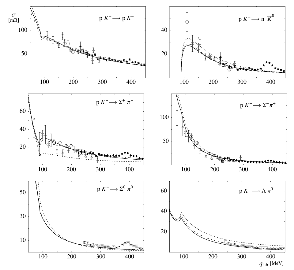
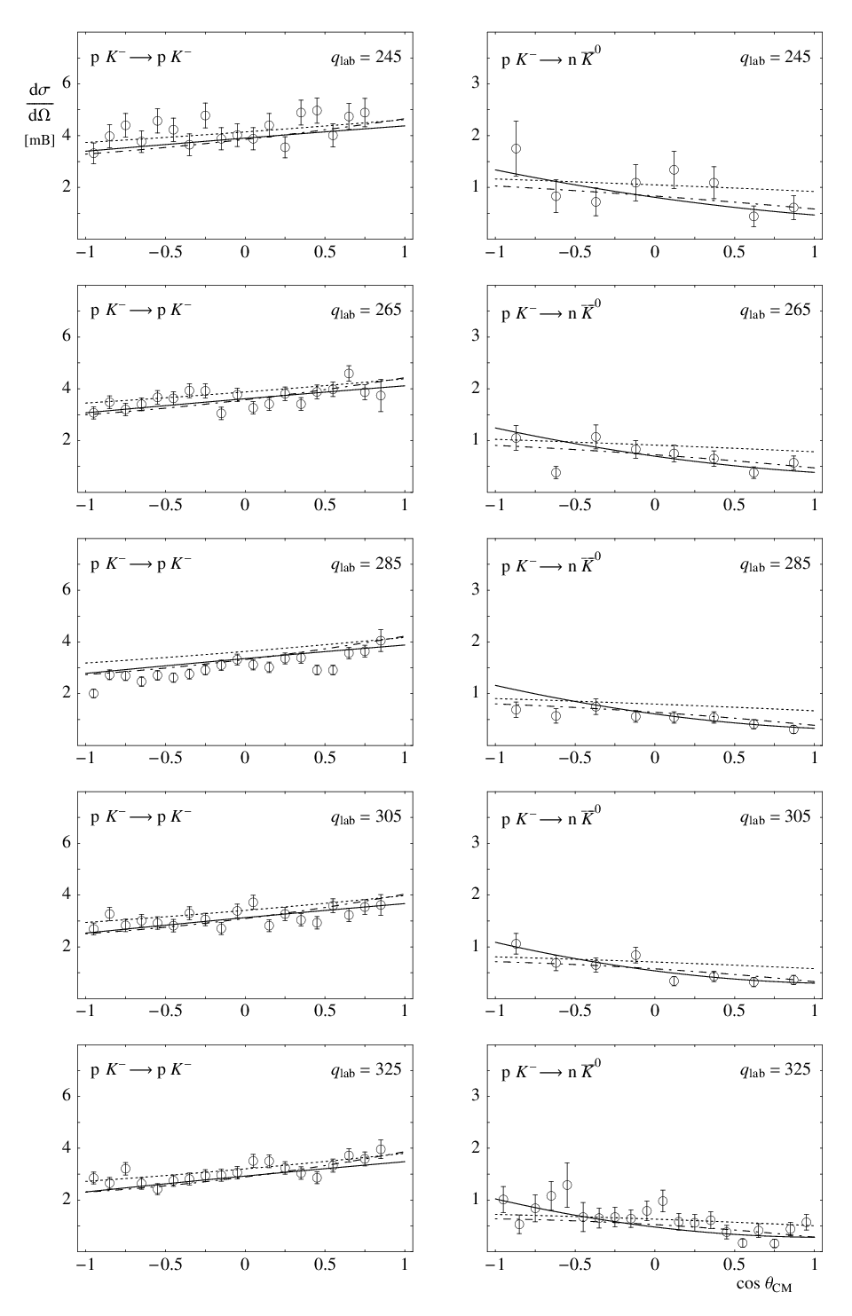
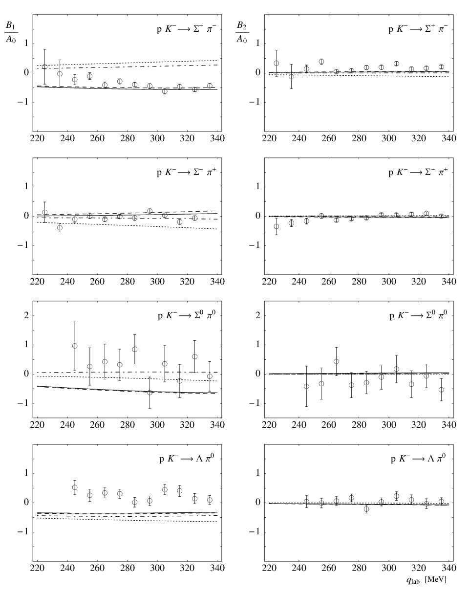
Our results for total cross sections are shown in fig. 1. As expected, fit III gives slightly better results than I. The contributions to the wave from - and -channel baryon octet exchange in those fits lead to a significan improvement over the results from NR. Fig. 2 shows our results for differential cross sections for . Although the difference between III and I is more marked in this case, with the latter giving a better description of data, all three curves shown in the figure provide a good description of data within experimental errors. The results for differential cross-section Legendre moments are significantly different for the three fits shown in fig. 3. As expected, parameter set I yields substantially more accurate results than III, NR, which were not fitted to this data. Results from fit II were omitted from these figures for clarity, since they are virtually identical to those from I.
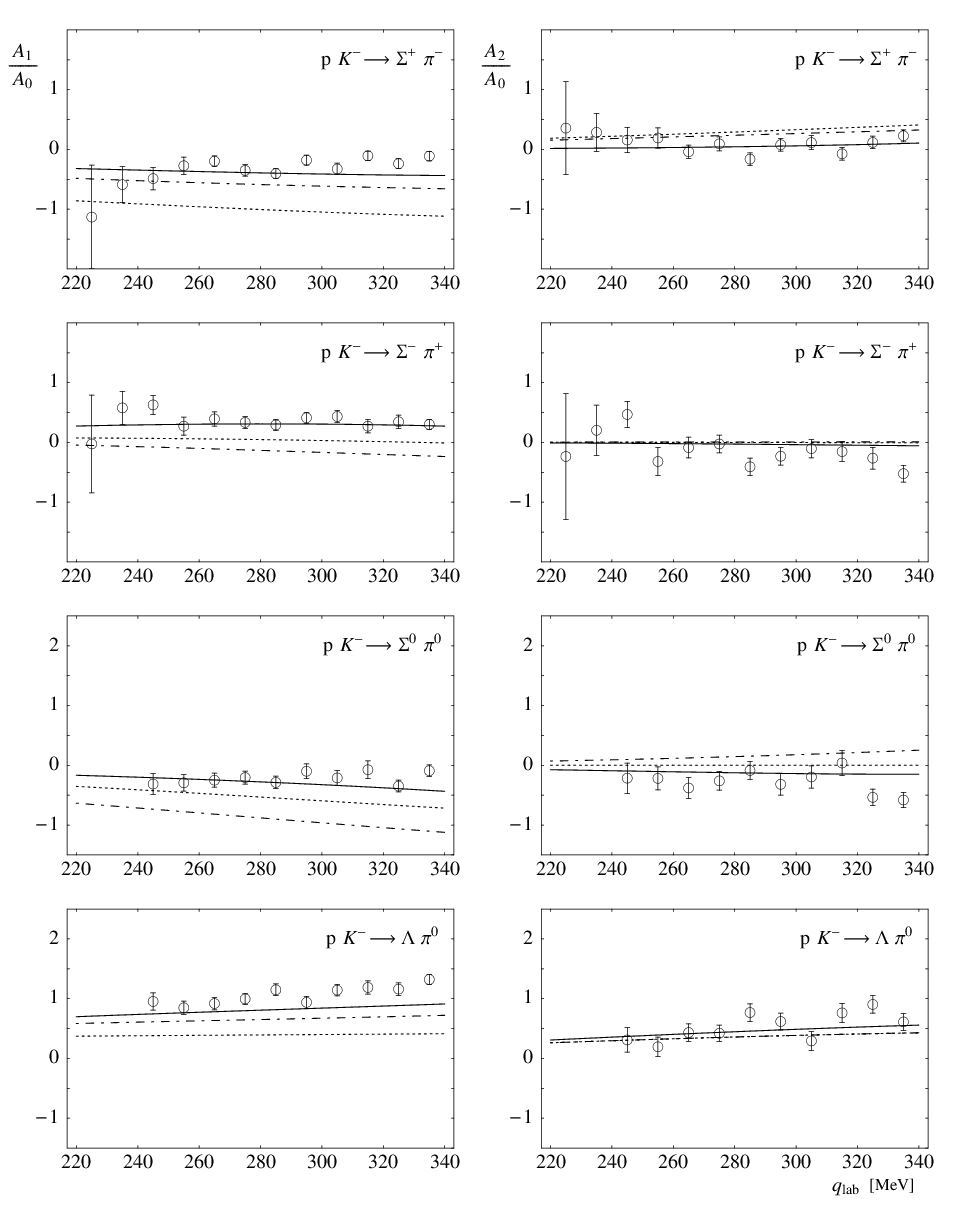
Fig. 4 shows our results for the Legendre moments of the CM-frame spin asymmetry. Fits I and II give a much better description of data than III and NR, as expected since the latter two do not include these data. The agreement of the former two with data is excellent for the charged modes . For the moment in all data points have a positive central value, whereas all four fits yield slightly negative values. This phenomenon is seen also in fig. 8 of [7], where results very similar to our fit I are obtained with the same experimental data. Clearly, new data would help resolve this issue. 33 3 Also, in [7] the data for for appear reflected through the horizontal axis. Such reflection would bring our fits I and II to a much better agreement with data. Still, given the large errors in these data, they have a small influence on fits.
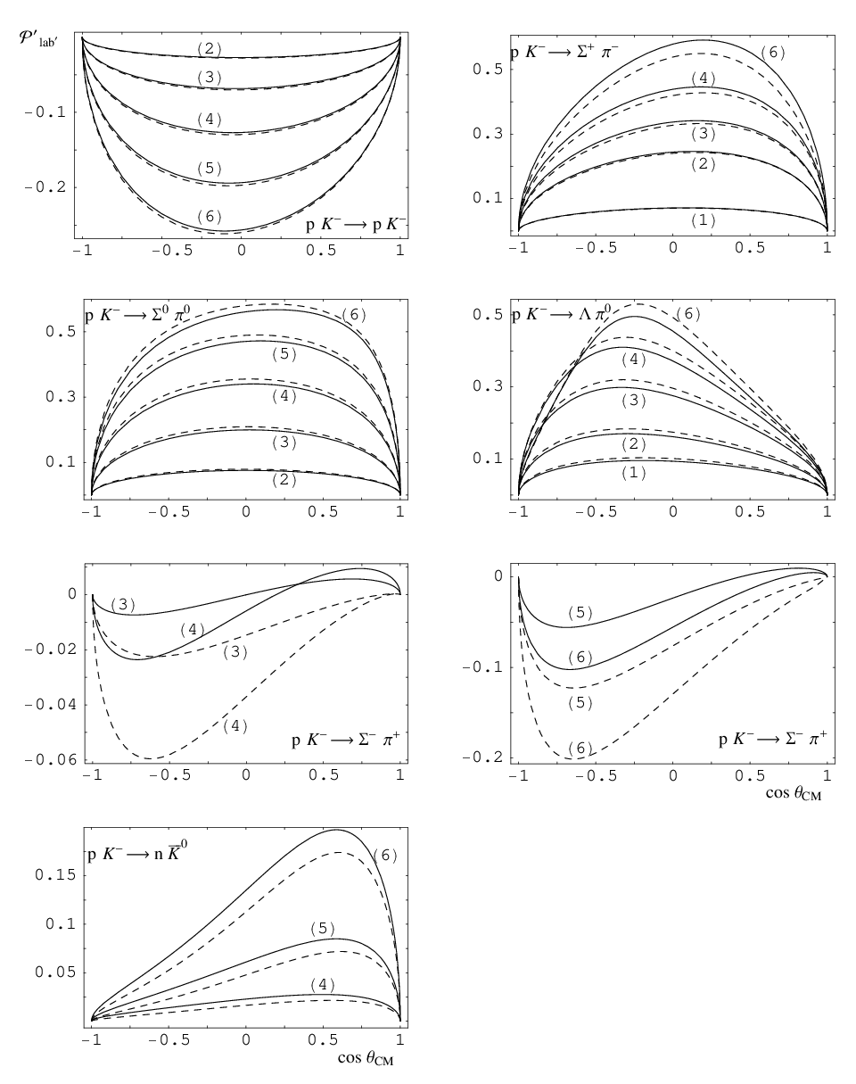
We show our results for final baryon polarization in fig. 5. Only results for fits I and II are shown, since only those give a good description of the spin-asymmetry data in fig. 4. As seen in the figure, there are small quantitative differences in the results for from I and II for , , and slightly larger ones in , . We take those differences as a rough estimate of the uncertainty in our results.
In the process there is a global sign change in : at low values of takes small but negative values over the entire range of , which change to positive values around MeV. We do not plot polarization values below 1%, so that sign change is not visible in the figure. As shown there, the difference between curves I and II is larger in this case than in the processes mentioned above.
A more marked sign change of is seen in the plots for , with small positive polarizations at small turning negative at 150–200 MeV. As is clear from the figure, this type of rapid evolution of with energy is sensitive to the parameters and not predicted reliably within the present approximation. Taking into account both higher order corrections in the perturbative amplitudes and higher partial waves in the unitarized ones would allow us to take into account higher energy data (up to 500 MeV if waves are included [7]). This would result in tighter constraints on the energy dependence of amplitudes and, presumably, reduce the uncertainties in the extrapolation to lower energies.
4 Results for scattering
No -channel interactions or resonance formation are present in scattering. Associated production of occurs about MeV above threshold in the CM frame, with the rest mass of at the peak at MeV, so it can be safely neglected in the range MeV considered here. We do take into account -channel exchange, though its contributions can be expected to be small. We use the , and partial waves from contact and -channel meson–baryon interactions, and from -channel decuplet baryon exchange, at tree level as input for one-channel unitarization.
The unitarized partial waves have four free parameters, the common pseudoscalar meson decay constant , the subtraction constant , and the couplings and from decuplet baryon interactions, which are obtained from fits to differential and total cross section data [43] for MeV. Our best fit to these data is obtained for MeV, , , and . This value of is slightly larger than that obtained in the previous section. Almost equally good fits are obtained for values of about 10 MeV higher or lower, with corresponding changes in the other parameters.
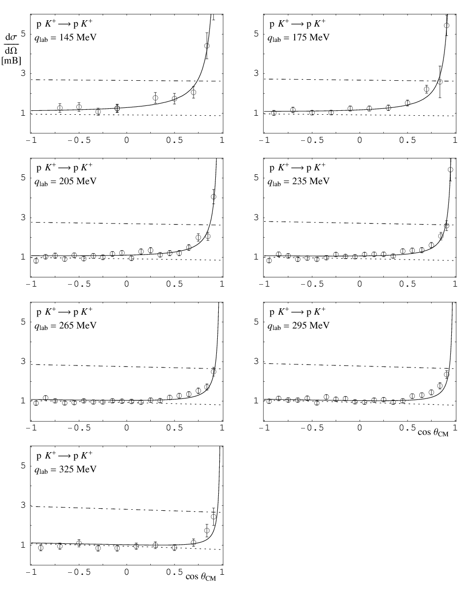
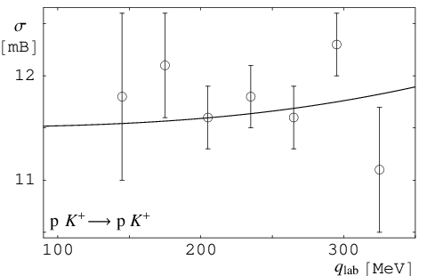
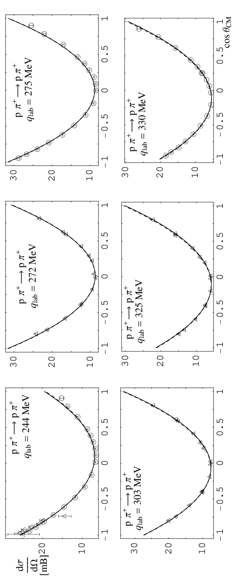
Results for differential cross sections for 145 325 MeV are shown in fig. 6. We corrected our UBChPT partial waves for final-state Coulomb interaction with the Coulomb amplitudes of [44] (see also [7]). The agreement with data is excellent. Also shown in the figure is the differential cross section from Coulomb-uncorrected UBChPT amplitudes, and from tree-level level amplitudes including neither decuplet baryon nor Coulomb interactions. As expected, the contribution from -channel baryon decuplet interactions is very small at these energies: setting =0 leads to barely visible changes in the figure. Total cross-section data is shown in fig. 7.
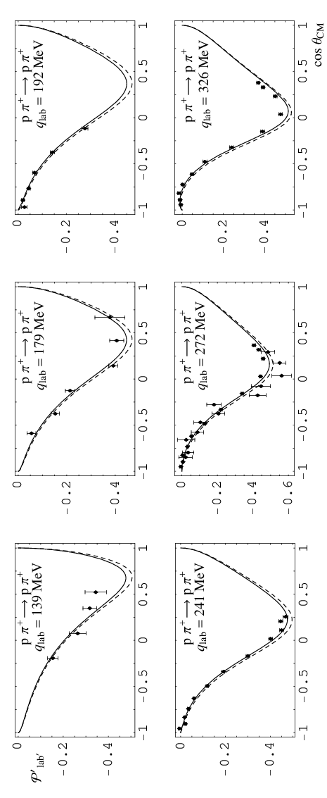
Results for polarization are shown in fig. 8. As expected, the effect of the Coulomb interaction is to erase polarization, and it is stronger at lower and in the forward direction. Also shown in the figure are the UBChPT results without baryon-decuplet contributions, and the result from leading-order BChPT (without both decuplet baryon and Coulomb interactions) for [15]. As seen in the figure the contribution to from exchange is small, about % of the polarization value at the higher end of the energy range in the figure and smaller at lower energies. The agreement between Coulomb-uncorrected UBChPT without decuplet baryons and leading-order BChPT results is remarkably good up to MeV, where higher-order correction effects become apparent. The fact that the UBChPT polarization is well approximated by the leading-order one at low energies shows that the former scales with approximately as , as the latter does exactly.
5 Results for scattering
scattering at low energies, 100 MeV, is well described by one-loop HBChPT [45]. Inclusion of degrees of freedom extends the applicability of HBChPT up to 300 MeV, as shown in [46]. Unitarization, and inclusion of the and meson, allows further extension to 400 MeV [10]. In the context of fully relativistic BChPT the interaction has been studied at one-loop level in [47]. No detailed phenomenological analyses of processes such as [45, 46] have been given in one-loop BChPT yet. In this section we apply the unitarized tree-level BChPT partial waves given above to scattering. At near-threshold energies, tree-level UBChPT is necessarily less precise than a full one-loop treatment. As discussed below, however, it yields a very good description of data up to 350 MeV, with many fewer free parameters.
For simplicity we restrict ourselves here to scattering. Besides the elastic process, also should in principle be considered. Unitarity corrections arising from the couplings of those channels, separated by more than MeV in the CM frame, are expected to be negligible at the energies considered here. Indeed, if that were not so the applicability of BChPT to scattering would be called into question. We therefore apply a one-channel unitarization procedure to the elastic amplitude, analogous to the treatment of scattering above.
We unitarize the tree-level partial waves , , computed from contact, - and -channel meson-baryon diagrams, and - and -channel exchange. The free parameters are determined from a fit to differential cross-section and analyzing power data in the region 150 330 MeV, around and below the resonance. A series of fits was performed in order to check the stability of our results, with only small differences found among them. The parameter , in particular, was found to be around 0.4 in all cases, with small fluctuations [10]. Using only differential cross section data, the best fit is found for
| (33) |
with a bare mass 1285 MeV. We refer to this fit as “I” below. For elastic processes lab-frame analyzing power is equal to lab′-frame polarization, as can be easily checked (see, however, [48] for an exhaustive discussion of polarization observables). Including analyzing power data in our fits we find,
| (34) |
with a bare mass 1299.5 MeV. We refer to this fit as “II”. The values for obtained in these fits is lower than the one from fits to data above, which may be explained by the fact that only interactions are present in this case. With respect to the value of the same caveats as in sect. 3 apply here. The resonance peak in the wave is located at 1226 MeV, with a Breit-Wigner width of 110 MeV, in both cases I and II.
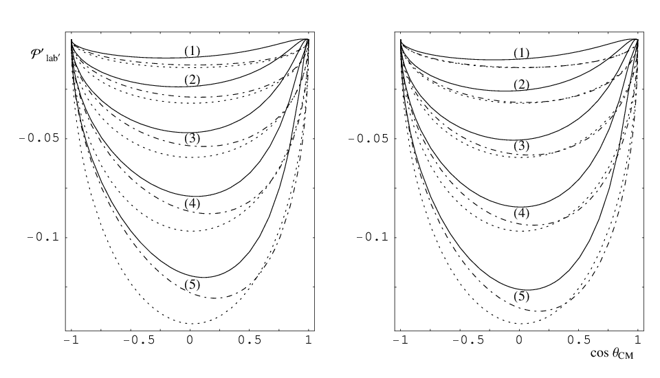
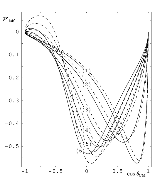
The resulting differential cross sections are plotted in fig. 9 for 350 MeV. Only a representative sample of data is shown in the figure, including only the energies with the largest number of data points, since the entire set comprises twenty different values of . The agreement with data is excellent, given the small experimental errors especially in the most recent experiments [49]. For these data the difference between I and II is barely visible in the figure. Polarization results are shown in fig. 10 to be in very good agreement with data.44 4 Notice that we define polarization in lab frame with respect to [15], so a sign-flip has been applied to the experimental data in fig. 10. The difference between the two fits is noticeable here at peak polarizations. Aside from that small difference, the result I is remarkable since polarization data were not included in that fit.
If we neglect decuplet baryons, the results from UBChPT agree quite precisely with those of leading order BChPT [15] up to MeV, similarly to the case of scattering discussed above. Inclusion of degrees of freedom leads to large effects. A comparison of results with and without was given in [15], where only the pole term in the wave was taken into account. The polarizations shown in fig. 11 are substantially larger than those in [15]. The latter are reproduced in the present approach if, firstly, we increase the value of (here extracted from data) to the larger nominal value used in [15]. And, second, if we restrict the -exchange contribution to -channel wave as done in that ref. The contribution of -channel exchange to the partial wave, in particular, is responsible for the enhancement of polarization with respect to [15] not accounted for by the change in . As shown in fig. 11, the contribution of -channel exchange to is comparatively small, except near the backward direction at the highest energies plotted there. Together with the results of [15], those presented in this figure give a complete picture of -resonance contributions to nucleon polarization at low energies.
6 Final remarks
In this paper we computed the polarization of the final-state baryon in its rest frame in low-energy meson–baryon scattering with unpolarized initial state, in the unitarization framework of [10, 11, 12] applied to fully relativistic leading-order BChPT.
For scattering very good agreement is found between UBChPT and unpolarized cross section data, confirming (and to some extent, improving) several previous analyses [11, 12, 16]. The agreement with CM-frame spin-asymmetry data is also good, though somewhat less certain, as seen in fig. 4. We attribute this to the scarcity of such data and the rather large errors in some of the existing measurements. On the other hand, it is precisely spin observables that put the tightest constraints on fit parameters, since the clearest discrimination among our different fits is provided by fig. 4.
The results in fig. 5 show large values of polarization for , even at relatively low energies ( MeV). It is interesting also that sizable polarizations are obtained for the elastic and quasielastic processes , at the upper end of the energy range considered in fig. 5. The stability of the results, as indicated by the two curves in fig. 5, varies widely for the different processes. Whereas the results for , , , final states seem reliable, those for are less stable, and for largely inconclusive. New, more precise data on unpolarized differential cross sections at low energies would certainly be most helpful to reduce uncertainties. Alternatively, as mentioned in sect. 3, extending the theoretical computation to fit the more abundant higher-energy data (along the lines of [7]) could lead to a more tightly constrained extrapolation to lower energies.
For scattering excellent agreement between our UBChPT results and differential cross-section data is shown in fig. 6. Significant ( 10%) values of polarization are found at the upper end of the energy range of fig. 8, even after correcting for Coulomb interaction. The agreement of the UBChPT result for polarization with that of leading-order BChPT [15] in fig. 8 is quite remarkable for MeV. Since those calculations were carried out by very different methods, their agreement provides a cross-check for both. Experimental data at these energies would obviously be most desirable.
In the case of scattering also excellent agreement is found with differential cross-section data in the peak region, as (partially) shown in fig. 9. Such agreement is remarkable given the high precision of some of the data sets used, and the fact that our results are based on unitarized tree-level amplitudes. More importantly, our results for polarization are in very good agreement with experimental data, as seen in fig. 11, which provides a non-trivial validation to our calculations.
Interestingly, a comparison of fig. 11 with the results of [15] shows that the non-resonant -wave contribution from -channel exchange has a strong influence on polarization, suggesting that precise polarization data could discriminate among different -- interaction models. As also shown in the figure, the contribution to polarization from -channel exchange, though significant, is relatively small.
We hope that the results presented here may motivate new measurements at low energies, or re-analyses of existing data, leading to new and more precise experimental information on polarization observables especially in the strange sector.
Acknowledgement
I thank the first referee for providing helpful information on analyzing powers and polarization.
References
- [1] V. Bernard, Chiral Perturbation Theory and Baryon Properties, arXiv:0706.0312.
- [2] S. Scherer, M. R. Schindler, A Chiral Perturbation Theory Primer, lectures given at the European Centre for Theoretical Studies in Nuclear Physics and Related Areas, Trento, Italy, 2005; arxiv:hep-ph/0505265.
- [3] P. Siegel, W. Weise, Phys. Rev. C 38 (1988) 2221.
- [4] N. Kaiser, P. B. Siegel, W. Weise, Nucl. Phys. A 594 (1995) 325.
- [5] N. Kaiser, T. Waas, W. Weise, Nucl. Phys. A 612 (1997) 297.
- [6] E. Oset, A. Ramos, Nucl. Phys. A 635 (1998) 99.
- [7] M. Lutz, E. Kolomeitsev, Nucl. Phys. A 700 (2002) 193.
- [8] B. Borasoy, E. Marco, S. Wetzel, Phys. Rev. C 66 (2002) 055208.
- [9] J. A. Oller, E. Oset, Phys. Rev. D 60 (1999) 074023; J. A. Oller, E. Oset, J. R. Peláez, Phys. Rev. D 59 (1999) 074001.
- [10] U. G. Meissner, J. A. Oller, Nucl. Phys. A 673 (2000) 311.
- [11] J. A. Oller, U. G. Meissner, Phys. Lett. B 500 (2001) 263.
- [12] D. Jido, E. Oset, A. Ramos, Phys. Rev. C 66 (2002) 055203.
- [13] D. Jido, J. A. Oller, E. Oset, A. Ramos, U.-G. Meissner, Nucl. Phys. A 725 (2003) 181.
- [14] J. A. Oller, Eur. Phys. J. A 28 (2006) 63.
- [15] A. Bouzas, Int. J. Mod. Phys. E, to appear.
- [16] E. Oset, A. Ramos, C. Bennhold, Phys. Lett. B 527 (2002) 99, Erratum: Phys. Lett. B 530 (2002) 260.
- [17] J. F. Donoghue, E. Golowich, B. R. Holstein, Dynamics of the Standard Model, Cambridge Univ. Press, New York, 1994.
- [18] J. Gasser, H. Leutwyler, Ann. Phys. (N.Y.) 158 (1984) 142.
- [19] J. Gasser, H. Leutwyler, Nucl. Phys. B 250 (1985) 465.
- [20] A. Krause, Helv. Phys. Acta 63 (1990) 3.
- [21] M. Frink, U. G. Meissner, J. High Energy Phys. 0407 (2004) 028.
- [22]
J. A. Oller, J. Prades, M. Verbeni, J. High Energy
Phys. 0609 (2006) 079,
Erratum: arxiv:hep-ph/0701096. - [23] J. Gasser, M. E. Sainio, A. Svarc, Nucl. Phys. B 307 (1988) 779.
- [24] M. Abramowitz, I. Stegun, “Handbook of Mathematical Functions,” Dover Pub., New York, 1972.
- [25] V. Bernard, N. Kaiser, U.-G. Meissner, Int. J. Mod. Phys. E 4 (1995) 193.
- [26] M. Benmerrouche, R. M. Davidson, N. C. Mukhopadhyay, Phys. Rev. C 39 (1989) 2339.
- [27] M. G. Olsson, E. T. Osypowski, E. H. Monsay, Phys. Rev. D 17 (1978) 2938.
- [28] V. Pascalutsa, M. Vanderhaeghen, S. N. Yang, Phys. Rept. 437 (2007) 125.
- [29] R. F. Lebed, Nucl. Phys. B 430 1994 295.
- [30] F. E. Close, R. G. Roberts, Phys. Lett. B 316 (1993) 165.
- [31] B. Borasoy, Phys. Rev. D 59 (1999) 054021.
- [32] P. G. Ratcliffe, Phys. Rev. D 59 (1999) 014038.
- [33] D. Tovee et al., Nucl. Phys. B 33 (1971) 493.
- [34] R. Novak et al., Nucl. Phys. B 139 (1978) 61.
- [35] M. Iwasaki et al., Phys. Rev. Lett. 78 (1997) 3067; T. M. Ito et al., Phys. Rev. C 58 (1998) 2366.
- [36] G. Beer et al., Phys. Rev. Lett. 94 (2005) 212302.
- [37] U.-G. Meissner, U. Raha, A. Rusetsky, Eur. Phys. J. C 35 (2004) 349.
- [38] B. Borasoy, R. Nissler, W. Weise, Phys. Rev. Lett. 94 (2005) 213401.
- [39] J. A. Oller, J. Prades, M. Verbeni, Phys. Rev. Lett. 95 (2005) 172502.
- [40] B. Borasoy, R. Nissler, W. Weise, Phys. Rev. Lett. 96 (2006) 199201.
- [41] J. A. Oller, J. Prades, M. Verbeni, Phys. Rev. Lett. 96 (2006) 199202.
- [42] B. Borasoy, R. Nissler, W. Weise, Eur. Phys. J. A25 (2005) 79.
- [43] W. Cameron et al., Nucl. Phys. B 78 (1974) 93.
- [44] G. Giacomelli et al., Nucl. Phys. B 71 (1974) 138.
- [45] N. Fettes, U.-G. Meissner, Nucl. Phys. A 693 (2001) 693.
- [46] N. Fettes, U.-G. Meissner, Nucl. Phys. A 679 (2001) 629.
- [47] C. Hacker, N. Wies, J. Gegelia, S. Scherer, Phys. Rev. C 72 (2005) 055203.
- [48] G. G. Ohlsen, Rep. Prog. Phys. 35 (1972) 717.
- [49] M. M. Pavan et al., Phys. Rev. C 64 (2001) 064611.
- [50] T. S. Mast et al., Phys. Rev. D 11 (1975) 3078.
- [51] M. Sakitt et al., Phys. Rev. 139 (1965) B719.
- [52] D. Evans et al., J. Phys. G 9 (1983) 885.
- [53] J. Ciborowski et al., J. Phys. G 8 (1982) 13.
- [54] T. S. Mast et al., Phys. Rev. D 14 (1976) 13.
- [55] R. O. Bangerter et al., Phys. Rev. D 23 (1981) 1484.
- [56] A. Stanovnik et al., Phys. Lett. B 94 (1980) 323.
- [57] P. J. Bussey et al., Nucl. Phys. B 58 (1973) 363.
- [58] B. G. Ritchie et al., Phys. Lett. B 125 (1983) 128.
- [59] M. E. Sevior et al., Phys. Rev. C 40 (1989) 2780.
- [60] C. Amsler et al., Lett. Nuov. Cim. 15 (1976) 209.
- [61] R. Meier et al., Phys. Lett. B 588 (2004) 155.
Appendix A Kinematics
In this appendix we gather some kinematical definitions used throughout the paper. We introduce the notation
| (35) |
The function appears frequently in relativistic kinematics (e.g., in the center of mass frame ). The Mandelstam invariants for the process are
| (36) |
with . The physical region for the process is defined by the inequalities
| (37) |
where,
| (38) | ||||