SLAC-PUB-13426
SU-ITP-08/32
Constructing the Tree-Level Yang-Mills S-matrix Using Complex Factorization
Philip C. Schuster1, Natalia Toro2
1 Theory Group, SLAC National Accelerator Laboratory,
Menlo Park, CA 94025, USA
2 Stanford Institute for Theoretical Physics, Stanford University,
Stanford, CA 94305, USA
A remarkable connection between BCFW recursion relations and constraints on the S-matrix was made by Benincasa and Cachazo in 0705.4305, who noted that mutual consistency of different BCFW constructions of four-particle amplitudes generates non-trivial (but familiar) constraints on three-particle coupling constants — these include gauge invariance, the equivalence principle, and the lack of non-trivial couplings for spins . These constraints can also be derived with weaker assumptions, by demanding the existence of four-point amplitudes that factorize properly in all unitarity limits with complex momenta. From this starting point, we show that the BCFW prescription can be interpreted as an algorithm for fully constructing a tree-level S-matrix, and that complex factorization of general BCFW amplitudes follows from the factorization of four-particle amplitudes. The allowed set of BCFW deformations is identified, formulated entirely as a statement on the three-particle sector, and using only complex factorization as a guide. Consequently, our analysis based on the physical consistency of the S-matrix is entirely independent of field theory. We analyze the case of pure Yang-Mills, and outline a proof for gravity. For Yang-Mills, we also show that the well-known scaling behavior of BCFW-deformed amplitudes at large z is a simple consequence of factorization. For gravity, factorization in certain channels requires asymptotic behavior .
1 Introduction
Gauge theories represent a highly constrained framework for describing interacting spin-1 particles. Weinberg’s seminal papers of 1964-65 [1, 2, 3] demonstrated that many of these constraints can be seen as inevitable consequences of requiring scattering amplitudes to be both unitary and Lorentz-invariant. In particular, both charge conservation and Maxwell’s equations follow from S-matrix arguments alone. Likewise, consistency of the spin-2 S-matrix requires the equivalence principle and Einstein’s equations at tree-level.
A concrete and beautiful confirmation that much of the structure of gauge and gravity theories is contained in their S-matrix is the existence of purely on-shell recursion relations for gauge theory [4, 5] and gravity [6, 7, 8, 9], which allow the calculation of on-shell scattering amplitudes entirely in terms of lower-point on-shell amplitudes. However, these relations have always been derived from the underlying local field theories; their relation to S-matrix consistency arguments such as [1, 2, 3] were unclear.
A striking connection between BCFW recursion and consistency of the spin-1 and spin-2 S-matrix was uncovered by Benincasa and Cachazo [10]. These authors introduced a “four-particle test”— the requirement that two BCFW shifts generate the same answer for any four-point amplitude. This requirement could only be met when the “coupling constants” (coefficients of three-point amplitudes) satisfied non-trivial relations. For instance, it was shown in [10] that the four-particle test generates the Jacobi identity for spin-1 particles. However, the four-particle test only makes sense when each of the BCFW constructions involved is valid (i.e. field theory amplitudes vanish in the limit of large shifts). The constraints obtained are reminiscent of those identified by Weinberg as consequences of Lorentz invariance and unitarity. The physical origin of the constraints obtained in [10] is somewhat unclear, however, as the argument assumes the validity of BCFW constructions. An open question in [10] was whether new constraints would be found by applying the same criterion to higher-point amplitudes. This question is also considered in [11].
After a brief review of the spinor-helicity formalism and BCFW recursion in Section 2, we show in Section 3 that the conditions from the four-particle test can be understood as the result of demanding Lorentz invariance and an analytic continuation of unitarity to complex momenta, “complex factorization”. The latter is simply the requirement that amplitudes factorize into sub-amplitudes when an intermediate complex momentum can go on-shell. A byproduct of this treatment is a simple criterion for BCFW shifts — shifts of the type (the only invalid shift in gauge theories) cannot possibly satisfy complex factorization in all limits.
BCFW recursion relations provide a formula for generating a set of arbitrary high-point amplitudes for spin-1 massless interacting particles. In Section 4 we show that amplitudes generated by BCFW recursion are guaranteed to satisfy complex factorization, provided the four-particle consistency requirements on couplings and shifts are satisfied. We also provide an S-matrix derivation of the large- scaling of BCFW amplitudes (as for deformations and for all others), which is used in our factorization argument. Thus, we have taken the programs described above fully on-shell: conditions on the structure of spin-1 amplitudes, and a construction of higher-point amplitudes from lower-point ones are justified with no reference to a local gauge theory.
We also outline the analogous result for gravity, and highlight the differences. One piece of the proof is missing: the argument relies on the scaling behavior of -point spin-2 amplitudes at large BCF shift parameters (i.e. growing as for shifts, and falling as for all others); an on-shell proof of this scaling result would complete the proof of factorization for BCFW gravity amplitudes.
2 Review of Formalism and Notation
In this section, we review two essential elements of the constructions in the remainder of this paper: the spinor-helicity formalism [12, 13, 14, 15] and BCFW recursion relations [5, 4, 16, 17]. The spinor-helicity formalism will be useful as a means of writing down manifestly Lorentz-invariant amplitudes for higher-spin massless particles, involving only the physical interacting degrees of freedom. BCFW recursion will be used as a means of generating amplitudes that satisfy unitarity in a subset of poles; however, the amplitudes thus constructed are not manifestly unitary in all limits — demanding unitarity in all remaining channels will give constraints on the fundamental three-particle couplings and on the set of allowed BCFW shifts, as discussed in Section 3.
2.1 Spinor-Helicity Formalism and Three-Point Amplitudes
Any four-vector can be related to a bispinor by ; when , has rank one, and we can write . The spinors and are uniquely determined by , up to a complex rescaling , and they transform in the and representations of the Lorentz group; they also transform simply under helicity rotations, . In this notation, two-particle momentum invariants can be written as
| (1) |
momentum conservation is the bi-spinor condition
| (2) |
and the Schouten identity
| (3) |
follows from the antisymmetry of spinor products and the fact that spinors live in a two-dimensional vector space.
The transformation properties of , under both Lorentz transformations and little group helicity rotations make them very useful for formulating an on-shell theory of spin-s particles — all of the Lorentz transformation properties of states are neatly encoded in the spinors. The helicity rotation operator associated with any external momentum is
| (4) |
Lorentz-invariant of an -point amplitude in which the ’th particle has helicity is guaranteed if
| (5) |
for all legs, and has no free spinor indices. Amplitudes are then naturally expressed in terms of Lorentz invariant “holomorphic” spinor products and “anti-holomorphic” products .
In fact, demanding the helicity transformation properties above fixes three-particle amplitudes completely up to coupling coefficients [10]. Note that the on-shell condition for three particles can be satisfied in two ways, either or ; though all real momentum invariants vanish in this limit, the spinor products can be non-zero in the first case, as can in the latter case. For example, a theory of several interacting massless spin-s particles has three-particle amplitudes (fixed by Lorentz invariance),
| (6) |
where refers to helicity, indexes label species of particles, and label four-momentum spinors. Demanding the amplitudes have crossing symmetry and are invariant under exchange of states requires the be completely anti-symmetric [10]. Under parity, and are exchanged. Demanding that pure spin-s interactions be invariant under parity requires , an assumption that we’ll make throughout this paper. To minimize the complexity of notation, we will often use the spinor labels to refer to species labels. There is another set of three-particle amplitudes and consistent with Lorentz invariance; however we will assume their coefficients are zero.
For later use, we also note the three-particle amplitudes for one spin-s particles with a collection of scalars:
| (7) |
where we have again assumed a parity, and labels species of scalars. In this case as well, the should be anti-symmetric in in order for the amplitudes to be symmetric under interchange of scalars.
2.2 BCFW Recursion
The BCFW formalism [5, 4, 16, 17] can be expressed very concisely in spinor-helicity formalism, but we first summarize it directly in four-momentum space. Consider the amplitude , where labels helicity. The basic idea of the BCFW formalism is to deform amplitudes into a function of a single complex variable , and then re-express the amplitude in terms of residues.
The simplest complex deformation of the amplitude that keeps all momenta on-shell is a deformation involving only two external legs. Consider the legs and . Choose an arbitrary null four-vector such that . Then we can deform by,
| (8) |
which keeps and null. In the spinor-helicity language, this is satisfied by this isimplemented particularly easy to implement by , so that the BCFW shift only deforms one of the two spinors associated with each leg:
| (9) |
We will call this the shift. Since , any kinematic invariant is at most linear in . These deformation naturally make the full on-shell amplitude a function of ,
| (10) |
At tree level, is a rational function of and so is fully determined by its poles and behavior as .
If we assume tree-level factorization, the only poles in the amplitude arise from propagators going on-shell, and their residues are fully determined by lower-point amplitudes. If as , the amplitude is then fully determined by products of lower-point on-shell amplitudes. In this special case, we obtain the BCFW recursion relation [4, 5],
| (11) |
where the sum is over partitions of into two sets and , is the (generically non-null) momentum flowing out of the right factor before the BCF shift, and is the null momentum flowing out of the right graph after the BCF shift.
This expression transforms properly under all helicity rotations (4) () so long as the same is true of the lower-point amplitudes from which it is generated. Thus, Lorentz invariance of BCFW amplitudes is manifest.
3 Consistency of Four-Point Amplitudes
In this section, we study the structure of consistent four-point amplitudes for four massless particles, satisfying two conditions — Lorentz invariance and a strong version of tree-level unitarity in unconstrained complex momenta, which we will refer to as complex factorization. We begin by explaining the conditions in some detail, then build amplitudes for specific examples. The general pattern that emerges is that, for high-spin theories, Lorentz invariance and factorization in a subset of channels fully constrains the leading behavior of the amplitude (in the sense of power-counting). This amplitude will only be able to satisfy unitarity in the remaining channel(s) if the coefficients of different three-point amplitudes are related. 11 1 The authors thank N. Arkani-Hamed for suggesting this approach.
Our results are closely related to those of [10] (and very much motivated by that work), but we make a significantly weaker set of assumptions. Specifically, the authors of [10] find conditions that three-point amplitudes must satisfy if four-point amplitudes can be constructed by a BCFW recursion. Therefore, their argument relies on field-theoretic derivations of the validity of different BCFW shifts. Since our goal is to motivate the self-consistency of BCFW constructions independent of field theory, and find an S-matrix criterion for their validity, it is important that we do not assume this. However, it is easy to see that when the assumptions of [10] are satisfied, the two methods will give the same consistency conditions on three-point amplitudes.
3.1 Setup and Interacting Spin-1
We begin by setting up the constraints on four-particle scattering amplitudes from Lorentz invariance, and explaining the requirement of complex factorization. We will consider the amplitude for scattering of four spin-1 particles as an explicit example, and derive the Jacobi identity.
We first demand that the four-particle scattering amplitude be a Lorentz scalar, and tranform as a product of one-particle states under independent helicity rotations of each. This condition is easily imposed in the spinor-helicity formalism — the only non-vanishing scalar invariants (under Lorentz invariance and individual helicity rotations) are
| (12) | |||
| (13) | |||
| (14) |
If we define an arbitrary particular solution that transforms correctly under helicity rotations, then a general four-point amplitude has the form
| (16) |
for some function . It will be most convenient to choose an that is polynomial in the spinor-product invariants, but does not contain any Mandelstam scalar invariants. For example, for four spin-1 particles of helicities ,
| (17) |
The requirement of complex factorization is the familiar tree-level unitarity — when any sum of momenta in a diagram goes on-shell, it gives rise to a single pole, associated with splitting the diagram in two, e.g.
| (18) |
where we sum over all allowed intermediate helicities, and a possible species index (we will drop in much of the discussion). We give this familiar criterion a new name, because we will require it to hold at arbitrary complex momenta. We have seen already that for particles of non-zero spin, there are two distinct three-point amplitudes in different on-shell limits — an when and an when . If , then both and vanish in the real-momentum collinear limit, where and both go to zero. This is a more general complexification of momenta than the usual analytic continuation of the Mandelstam variables, and we will see in a moment that there are cases where a real-momentum limit is trivial, but one of the two complex directions is not.
Which three-point amplitudes appear in the unitarity condition 18 depends on how we take the limit . We can take either
| (19) |
or
| (20) |
The limit and also enforces either for all or a soft limit on one of the three legs; we will not demand unitarity in this limit. We can thus refer unambiguously to the two limits above as (19) or (20).
Having stated the requirement of complex factorization, let us apply it to the four-gauge-boson amplitude. One way of obtaining an expression that factorizes in the limits and is by using the BCFW formula, using a shift , (called a shift). The two terms in the formula are shown in Figure 1

The result is
| (21) |
where repeated indexes are summed. The fact that we have obtained this amplitude by a BCFW construction is quite incidental — it is the unique amplitude one can write down, involving only dimensionless coupling constants, that factorizes in the limits and and has no unphysical poles. For example, adding a term to the scalar function in brackets would introduce two single poles at unphysical locations, where no particle goes on-shell; adding a contribution would introduce an unphysical double singularity as , and of course adding a term or would change the - and -channel singularities.
One can check that the and singularities in (21) have the proper form, and they do. More interesting conditions come from the -channel. We note that, because of the helicity factor, (21) has a pole as but not as . In fact, the real limit with vanishing simultaneously also vanishes. But the limit is non-zero. Complex factorization (19) requires
| (22) | |||||
| (23) |
while above has
| (24) |
For the two expressions to agree, the couplings must satisfy a Jacobi Identity:
| (25) |
(where we’ve restored the full species label for clarity). This result was also found in [10], by demanding agreement of two BCFW shifts involving different legs. It is clear why these give the same result: the two BCFW shifts are imposing factorization in different poles!
We have now obtained a four-point amplitude that can satisfy complex factorization in all channels; it is unique up to less singular terms, which by power-counting must have new, dimensionful couplings. Writing down any such amplitude required a relation between three-point coefficients. With this amplitude in hand, we can now check BCFW recursion relations explicitly, with different shifts. We have already seen that the shift gives the correct amplitude; so do the shift and all shifts of legs with helicities , , or . However, if we try to build an amplitude with the shift, we find
| (26) |
This satisfies factorization in the and limits ( as and is non-singular as ), but has an unphysical fourth-power singularity as and no -channel singularities. So we can see directly that this shift cannot produce physical amplitudes. Our finding that all shifts except are valid agrees with the gauge-theory result [4, 5].
3.2 Spin-1 With Matter
We can repeat this analysis for spin-1 interactions interacting with massless matter (for simplicity, we consider scalars) labelled by indexes , with three-particle amplitudes given by equation 7. Consider the four-particle amplitude . We again use a shift to build an amplitude, and again it is consistent with factorization in both -channel limits and both -channel limits (though the factorization as does not follow from the BCFW construction, and must be checked explicitly):
| (27) |
Again, any modification with the same energy-scaling would violate complex factorization in the or -channels, or introduce unphysical singularities elsewhere. As , complex factorization requires
| (28) | |||||
| (29) |
and in this case the limit is identical. The limit of the BCFW construction is
| (30) |
which satisfies factorization if
| (31) |
(where we have again restored full species labels). We recognize this as the requirement that the furnish a representation of the Lie Algebra defined by the .
For self-interacting scalars with a three-point amplitude , we can apply -channel factorization to the amplitude constructed with an shift, and find that the scalar interaction must satisfy charge conservation. We do not show this explicitly here. One could also check using this amplitude or the previous one that at four-point, shifts and are valid but shifts or are not, consistent with the general field-theory result of [18].
3.3 Spin-2
We can repeat the above analysis for massless interacting spin-2 particles. First consider the amplitude constructed from a shift ( and labels and helicity states). Using the BCFW ansatz, we obtain,
| (32) |
Interestingly, each term separately has a double pole as (taking ). Complex factorization in this channel requires
| (33) | |||||
To make the double pole vanish, we require
| (34) |
(so that in the numerator cancels an in the denominator), while getting the correct coefficient on the single pole requires additionally
| (35) |
As pointed out in [10], these relations imply that the furnish an algebra that is commutative and associative, and therefore any multi-graviton theory can be reduced to a theory of self-interacting gravitons that decouple from one another. From here on, we will consider only one spin-2 species.
We next consider a single massless spin-2 particle coupled to a set of interacting scalars. As before, the fundamental three-particle scalar interactions are just constants . The fundamental spin-2-scalar three-particle amplitudes are
| (36) |
(by symmetry, the spin-2-scalar couplings must be symmetric in the , so we have diagonalized them). We now consider building the amplitude using a shift. The BCFW construction gives,
| (37) |
Demanding complex factorization in the channel requires,
| (38) | |||||
Again, there is a potential double pole. The double piece vanishes and the correct factorization limit is obtained provided . This is a special case of the principle of equivalence for gravity –interacting matter couples to gravity with the same strength.
4 Factorization of Higher-Point Amplitudes
In this section, we will show that -point amplitudes obtained by BCFW recursion satisfy the physical requirements of complex-momentum unitarity (factorization). We have already noted that Lorentz invariance is manifest in the construction, so long as the recursion begins from Lorentz-invariant primitive three-point amplitudes. We now describe the factorization requirement in more detail, for a theory of massless particles at tree-level.
In the limit that the summed momentum of a collection of legs, becomes null, unitarity requires that the amplitude have a single pole, whose residue is a product of two sub-amplitudes:
| (39) |
where is the set of legs not in , which must contain at least two legs (we can label the same limit equivalently by either or ). When contains only two legs,
| (40) |
goes to zero if either or ; for complex momenta we can obtain limits in which one spinor product goes to zero while the other remains finite. This results in distinct factorization formulas, involving when and when .


The BCFW recursion singles out the two shifted legs, which we will label 1 and 2, and treats different poles differently. The BCFW formula (11) manifestly satisfies the factorization requirement (39) in each of the poles that appears in the sum, namely for some set of legs . The explicit propagator in the term of (11) with becomes singular. Nothing else in the BCFW expression can be singular in this limit — the sub-amplitudes are evaluated at shifted momenta, at which no kinematic invariants inside the sub-amplitudes vanish. If either side of the pole has only two elements, we must specify which spinor product is exposed by the BCFW shift: if has only one element , the BCFW shift exposes the pole , and if contains only the legs , the BCFW shift exposes the pole .
Factorization in the remaining poles, which correspond to kinematic invariants that do not depend on , must be verified explicitly. Checking that BCFW amplitudes factorize in these non-manifest limits is the main task of this section; we will demonstrate it by induction, assuming that -point amplitudes factorize. The arguments are somewhat technical, but contain surprising structure; we will highlight the pieces of the BCFW expression that do contribute to each singularities, and the structural properties of the amplitudes that are required for factorization. We now classify these poles, and summarize the properties required for their factorization.
We first consider poles where and contains at least one additional leg. Terms in the BCF sum for which or are singular in this limit; because the BCFW shift does not affect the kinematics of the legs in in any way, the inductive proof of Section 4.1 is straightforward, and independent of all details of the chosen amplitudes and BCFW shift. When contains only two legs, one subtletly will appear that requires the same relations between coupling constants seen in the four-point amplitudes of Section 3.
BCFW shifts leave two other types of invariant unaffected: (and ) and () for . Unlike those discussed above, factorization in these limits depends on the spins and helicities of the particles involved. The collinear singularity as arises in the BCFW formula from amplitudes where a soft BCFW-shifted leg 1 is attached to each of the un-shifted legs (Sec. 4.2). This limit is closely related to the soft-photon and soft-graviton limits considered by Weinberg [2]. For spin-1, color-ordering reduces the factorization statement to the equality of one soft and one collinear diagram or of two soft diagrams. The spin-2 factorization receives contributions from soft singularities in terms, each of which produces a double pole in ; the correct single pole of factorization is obtained using momentum conservation. Attempting to apply the BCFW recursion shifting legs with helicities , which is not a valid BCFW shift, we see that factorization cannot be satisfied.
The “wrong-helicity” factorization limit , which we discuss in Section 4.3, arises from multiple BCFW terms in both gauge theory and gravity. In gauge theory, their sum can be interpreted precisely as a BCFW construction of an -point amplitude. However, the helicities of the shifted legs in the -point amplitude can differ from those in the original -point amplitude, so for example the proof of factorization for shifts depends on the validity of shifts as well. The proof also depends on the large- scaling properties of amplitudes, in particular the vanishing of amplitudes as at large , and the growth of amplitudes under “invalid” shifts bounded by . A simple power-counting argument justifies this scaling for (see Appendix A), but we do not have a proof of this scaling for gravity, so the factorization argument in that case remains incomplete. As for the poles, factorization is violated for the invalid shifts, in this case by non-vanishing boundary terms.
4.1 Factorization on Unshifted Multi-Leg Poles
Let be a set of legs that excludes the shifted legs 1 and 2, and at least one other leg. Factorization requires that in the limit ,
| (41) |
where is the complement of in .
If contains three or more legs, this result is readily obtained by considering the limit as of the BCFW decomposition (11) of (one subtlety will arise in the two-particle case, discussed below). The only terms that are singular in these limits are those with or . Factorization of the left or right sub-amplitudes (the induction hypothesis) yields a simple limit:
| (42) |
where is the subset of not explicitly written; terms with in the right factor have analogous limiting behavior. In particular, all of these terms have a common factor , which is one of the factors of the desired -point factorization limit. Adding these terms, we find
| (43) | |||||
| (44) | |||||
| (45) | |||||
where in the last line, we have recognized terms (43) and (44) as a BCF formula for the lower-point amplitude . This argument is illustrated diagramatically in Figure 4.

Note that the argument above fails completely if contains only one and two — there are no diagrams in the BCFW sum for which or , and in fact, as we will see, very different terms are singular in that case, which we consider in Section 4.2. We first elaborate on the special case that the set contains only two particles (); in this case, one additional class of diagrams plays a role.
4.1.1 Two-Particle Unshifted Poles
For definiteness, we consider the singularity . In this case, one term in the BCFW expansion that we might expect to be singular is in fact non-singular, and two new terms are singular:
- •
- •
Two additional terms in the -point amplitude, not included in (45), are singular — those in which the left factor contains only two legs: and either 3 or 4. When legs and are alone in the left factor, for instance, the intermediate leg has , so that as we also have ; therefore, this term can be singular even though legs and are split between factors. The singularity of this term is given by
(47) where the factor in braces is obtained by factorization of the right BCFW factor. A similar term is obtained when legs 3 and 4 are exchanged.
We recall the argument for factorization in multi-particle poles: the factorization limits of every individual term in the -point BCF amplitude can be interpreted as a contribution to the BCFW formula for the lower-point ampitude appearing in (41). By the discussion above, there are two new terms in the BCFW ansatz that do not have this form. There is also a term that must appear in the BCFW formula (43-44) for the lower-point amplitude, but is not generated by factorizing any one term in the -point BCFW ansatz. This missing term is
| (48) |
(we maintain the conventions introduced earlier, that ’s denote summed momenta that become null in singularity limits, ’s unshifted intermediate momenta in the BCFW formula, and the null shifted intermediate momenta in BCFW).
To recover the correct factorization result, the extra terms in the factorization of the -point BCFW formula must compensate for the missing term — Eqn. (47) and its analogue with 3 and 4 exchanged must sum to (48). This is so, and follows from the Jacobi identity (spin-1) or equality of all couplings (spin-2). It is worth stressing that, although our result will be very reminiscent of the factorization of four-particle amplitudes in Section 3, it is not the same physical limit — indeed, the products do not arise as factorization limits of four-point amplitudes. In fact, these products are non-zero only for external helicities , for which the four-point amplitude vanishes.
To proceed, let us define
| (49) |
The ’s have a simple form:
| (50) |
where
| (51) |
depends only on the helicities of the particles (not on how they are paired), and is zero for all other combinations.
Terms (47) and (48) all have the limiting form
| (52) |
where is some ordering of , where is the limiting BCF-shifted momentum of leg in (48), and (all three terms approach this uniform kinematics as ). Factorization requires the coefficients of in (47) to reproduce the coefficients in (48), i.e.
| (53) |
By judicious use of kinematic identities, this can be rewritten as
| (54) |
which vanishes by the Jacobi identity for and the Schouten identity (setting all equal) for .
Thus, the non-standard terms (47) are equal to the term (48) that was missing from the naive sum, and factorization on poles like is guaranteed by the BCFW construction for both spin-1 and spin-2. An analogous result would hold when the opposite-helicity invariants , except that in that case, the roles of legs 1 and 2 are interchanged, and the identity involves anti-holomorphic 3-point amplitudes instead of holomorphic ones.
4.2 Factorization on “Unique Diagram” Poles ()
The BCFW formula does not contain any sub-amplitudes with “propagator” singularities as because, by construction, legs 1 and 2 are in separate factors and the remaining legs are split between the factors. Instead, the collinear singularities arises remarkably in the BCFW formula through a soft singularity in one of the factors. Specifically, whenever the left-hand factor in the BCFW decomposition (11) is a three-point amplitude for some leg , we find (analogously, in the limit, becomes soft when the right-hand factor is a three-point amplitude). The right factor, an -point amplitude, approaches a uniform kinematic limit for all , which is in fact exactly the kinematics that appears in the factorization formula:
| (55) |
The behavior of the three-point amplitude as depends on the helicity of the soft leg. If , all three-point amplitudes in (55) vanish as , so the BCFW sum is non-singular. This makes the factorization limit either trivial (when , the three-point amplitude in (55) is also zero) or manifestly violated (when , (55) is non-zero, but the BCFW formula cannot reproduce this singularity). The latter case corresponds to the shift , which we have already seen does not produce consistent four-point amplitudes.

If , the three-point amplitudes in (55) do have a soft singularity (they scale as ), and the factorization condition is non-trivial. In this case, the singularity of the BCFW amplitude is given by
| (56) | |||||
where we have written helicity and species indices explicitly in the three-point amplitude and for the modified leg in the -point amplitude.
We begin by describing the kinematics of (56) more explicitly to illustrate the soft limit, then consider the sums separately for the spin-1 and spin-2 cases. The shifted spinor in the ’th term is proportional to ; the constant of proportionality and the value of can be found by taking the inner product of with or , respectively:
| (57) |
We note that is indeed becoming soft (one can understand the limit as follows: as and become nearly proportional, a fine-tuned subtraction of nearly equal spinors is required to obtain a spinor ). Since is soft, the momentum leaving the -point factor must approaches :
| (58) |
and the shifted momentum of leg 2 is,
| (59) |
As we have noted, the limiting kinematics of the -point amplitudes as is independent of which leg appears in the left factor! In fact, it is the same kinematics that appears in the -point amplitude of (55). However, the line leaving the =point diagram in each case can have different internal species quantum numbers than those of the original outgoing line .
One might also expect the line to have different helicity than , but in fact these diagrams need never be considered. We have already noted that, if , the factorization requirement is either trivial (when ) or impossible to satisfy (); the non-trivial case is . But the gauge/gravity amplitude is only non-zero if its two remaining legs have opposite helicities, which in our notation is .
Before considering the singular three-point terms in more detail, we clarify why the generic case — in which the left factor is a higher-point amplitude, does not contribute. In this case, as , the shifted leg approaches a non-singular limit
| (60) |
where is the (generically non-null) sum of momenta of the legs in the left factor. As no momenta or invariants within either sub-amplitude vanish at this point, we expect no singularities. Likewise, no singularity occurs when the right-hand factor is three-point, because and the spinor by which it is shifted are not orthogonal.
4.2.1 Spin-1 Factorization
We now consider the three-point amplitudes in somewhat more detail for the theories of pure spin-1 “gauge-theory-like” (++- and –+) interactions. The kinematic factor times three-point amplitude in the ’th term (in parentheses in Eqn. (56)) is given by
| (61) |
Note that approaches an -independent, finite limit as , so different terms in the sum (56) differ only in the replacement of the ’th particle’s species index by a dummy label , and contraction into a coefficient . One can see that this identity holds by separately considering every contraction of many ’s that could appear in the -point amplitudes in (56), and repeatedly using the Jacobi identity.
It is much less cumbersome, however, to switch to the color-ordered formalism [19, 20, 21]. Because the cyclic ordering of leg indices is significant in color-ordered amplitudes, we will call the BCFW-shifted legs in this discussion rather than , to avoid suggesting that they are color-adjacent when they need not be. We have already seen that, for four-point spin-1 amplitudes to factorize, three-point couplings must satisfy a Jacobi identity. We can then associate each “species index” with an element in the adjoint representation of a Lie algebra; the relation on species indices described above is a trivial consequence of this structure. The only color structure ever generated in tree amplitudes is a single trace, allowing us to express any amplitude as a sum of color traces times colorless primitive (or color-ordered) amplitudes,
| (62) |
The color-ordered amplitude receives contributions only from diagrams in which the legs are cyclically ordered from 1 to clockwise on a plane, and all coefficients can be replaced with a uniform coupling constant . Aside from this, color-ordered BCFW amplitudes have the same structure as unordered ones. The color-ordering is, for our purpose, simply a bookkeeping device to focus on one color-structure (i.e. one set of contracted ’s) at a time using their known algebraic structure. This bookkeeping simplifies the discussion considerably: instead of diagrams, for a given color-ordering only two diagrams contribute to this discussion.
We must consider two cases separately: when the legs and are color-adjacent, and when they are not. If legs and are not color-adjacent, then no diagrams in which and connect at a three-point vertex have the correct color ordering, so there is no singularity as ; there are, however, two non-vanishing terms in the BCFW expression (56) (namely, ). These appear with opposite signs, since the color-ordering includes and (with no sign flip). Thus the two diagrams cancel, correctly giving no singularity.
If and are color-adjacent (for definiteness, say , ), the factorization limit (55) is non-zero:
| (63) |
and is reproduced exactly by the one non-zero term in the color-ordered BCFW expression (using (56) and antisymmetry of the three-point amplitude),
| (64) |
In each case, then, the color structure established at four-point and properties of three-point amplitudes suffice to guarantee the factorization of -point BCFW amplitudes as (the analysis for is analogous, with the roles of legs 1 and 2 exchanged).
4.2.2 Spin-2 Factorization
To study spin-2 interactions, we use the fact derived from spin-2 four-point amplitudes in [10] that interactions among spin-2 particles can always be written as self-interactions of a single species. Therefore, there are no species indices in (56), and the -point amplitudes approach truly identical limits. Unlike the case of spin-1, however, the kinematic three-point factors of (56) do depend on the ’th particle’s momentum — they are given by,
| (65) |
Moreover, the individual terms become singular as (i.e., since we are attempting to evaluate a residue, each BCFW term in fact has a double soft singularity as ). Replacing each of the -point amplitudes in (56) with its limiting kinematics, we find,
| (66) |
Writing,
| (67) |
the limit of (66) becomes,
| (68) |
By momentum conservation, the first sum in parentheses is identically zero and the second is equal to ; thus we recover the singularity limit,
| (69) |
In fact the argument above is a bit too quick: for small but finite , each -point amplitude in (56) is evaluated at slightly different kinematics; because the prefactors in (56) are themselves growing as , this displacement could change the final result by a non-zero amount. As we show explicitly in Appendix B, this correction has no effect at all on the limit –it is proportional to a sum over all legs of , which vanishes because is antisymmetric.
4.3 Factorization on Wrong-Factor Poles ()
The final class of factorization limits we must check is the limit for (the case for is analogous). We will consider concretely the limit (again, the sequence of labels is arbitrary). In this limit, we require
| (70) |
As before, we will prove this for -point amplitudes by induction, assuming that all lower-point amplitudes factorize appropriately and can be generated by the BCFW construction.
We will classify terms of the BCFW sum as in Figure 6 (we will mention only terms that have potential singularities). We will first consider terms (a), in which the left factor contains legs 1 and 3, and at least one additional leg — these will combine into an expression like (70), in which the -point amplitude has been expressed using BCFW recursion. Terms (b) and (c) will not contribute to the factorization limit, but to show this we will need to use the fact proved in Appendix A for spin-1, that at large shifts , -point amplitudes generated by BCFW have the same -scaling as 3-point amplitudes (i.e. for all “legal” BCFW shifts and no faster than for the “illegal” shift ).
The outline of this proof holds for gravity as well, but the sum of terms (a) will contain additional contributions, that only vanish if the -point amplitudes fall as under valid BCFW shifts. Likewise, the absence of singularities from terms (c) only vanish if multi-point gravity amplitudes have the same -scaling as 3-point amplitudes. We know this to be true of spin-2 BCFW amplitudes from analysis of the gauge-theory amplitudes [8, 9], but do not have an S-matrix argument for why it must be so.
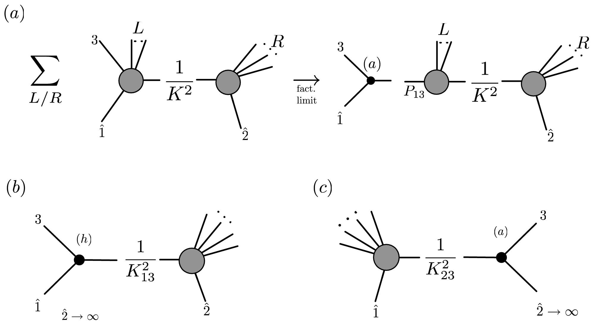
4.3.1 Terms (a)
Terms of the form (a) in Figure 6 are each evaluated at a different , but the shift does not change or . By the induction hypothesis, the left BCFW factor in each such term should factorize on the pole as,
| (71) |
The three-point amplitude in (71) vanishes if ; otherwise, it is non-zero. Writing as , we find . The power depends on the helicities but is the same for all terms; it is convenient to express all amplitudes in terms of the unhatted 3-point amplitude,
| (72) |
Substituting this form into (71) and summing over all such contributions to the BCFW formula, we obtain
| (73) | |||||
| (74) |
If =1, we recognize the sum in (74) as a BCFW formula for the -point amplitude in (70), obtained by a shift (note is the same as appearing above). Thus (74) reproduces the desired factorization limit (70), provided is a valid shift.
In general, the helicity of can differ from (for instance, if and then the only non-vanishing contribution in (74) comes from ). So the validity of factorization on poles for shifts depends on the validity of a lower-point BCFW formula using shifts . It is important to check that the above procedure never introduces the BCFW construction using a shift. Indeed, this would require an anti-holomorphic amplitude , which is absent from the theory. Thus the shifts valid at 4-point are a closed set.
Something surprising happens for the spin-2 () case: each term in the would-be BCFW sum is multiplied by . The 1’s combine into a BCFW-shifted amplitude, yielding the correct factorization limit as in the spin-1 case. However, the sum of terms proportional to remains. These are, however, simply the residues of (recall that the terms in the BCFW sum are residues of , and we have multiplied them by the ’s at which the poles occur)! therefore, the limit of our partial sum is given by
| (75) |
The contour integral at infinity vanishes when — this is a known property of gravity amplitudes [8, 9], but it is surprising from both their Lagrangian or recursive definitions (we will not prove it here). The appearance of this formula in the factorization requirement is mysterious, and suggestive that the scaling of gravity amplitudes is crucial for self-consistency of the theory.
4.3.2 Terms (b) and (c)
These are not the only terms in the BCFW sum that can be singular in the limit. We now consider two more potentially singular terms in the BCFW sum (which we expect to vanish, since we recovered the correct answer already from terms (a)):
| (76) |
and,
| (77) |
The contribution (76) has a net in the explicit propagator, but the 3-point amplitude is proportional to so (76) is not singular for . The term (77) has potentially singular behavior because the shifted momenta,
| (78) |
go to infinity as . The growing momentum is suggestive of a large- BCFW shift – a limit in which we expect lower-point amplitudes to approach zero. To make this explicit, we write the momenta and in a somewhat unusual way. We first define “initial” momenta,
| (79) |
note that as , these momenta approach limits and . The hatted momenta in (77) can be written as a BCFW shift of the “initial” momenta:
| (80) |
All invariants involving “starred” momenta are generically finite, and differ from invariants of “naught” only by terms supressed by . Therefore, the scaling of the -point amplitude in (77) as is dictated by the large- scaling of
| (81) |
which we derive for spin-1 in Appendix A. Using this result and the explicit kinematics of (78) for the three-point amplitude, we find that, as long as is a “valid” BCFW shift, (77) is non-singular as . This is summarized in Table 1. We highlight three examples:
- •
If and , then the only non-zero term comes from . The three-point amplitude diverges as , but the scaling of the -point amplitude under a large shift is , so the product has a finite limit.
- •
If instead , then the 3-point amplitude vanishes as , but the -point amplitude grows as under a shift; again the product approaches a finite limit as .
- •
For “invalid” BCFW shifts , term (c) does contribute a singularity (in fact, an unphysical multiple pole!). For example, we consider the contribution from when and . The three-point amplitude in (77) scales as and the -point amplitude scales as under the shift – as , the product can have an unphysical singularity!
| -point | Three-point | Total scaling | ||||
| + | + | + | - | |||
| + | + | - | + | |||
| - | + | + | - | |||
| - | + | - | + | |||
| - | - | + | + | |||
| - | - | - | X | (c) vanishes identically | ||
| + | - | + | + | |||
| + | - | - | X | (c) vanishes identically | ||
The scaling of gravity amplitudes is known to be the square of the gauge theory scaling described above – this scaling suffices to guarantee that the term (77) does not contribute to the factorization limit in gravity, either. However, unlike gauge theory, we have not found an S-matrix argument for why this must be so. The pivotal role of scaling in showing that gravity amplitudes factorize is striking and unexpected — this is a faster scaling than is required to prove BCFW in field theory, for example! It is possible that in some cases, the boundary-term of (75) cancels the one arising from (77). But such a cancellation is unlikely to be universal. For example, if and , the boundary term of (75) is associated with a coefficient of in a falling amplitude, while (77) is the product of a growing -point amplitude with a 3-point amplitude that falls as !
5 Summary and Remarks
The BCFW recursion relation is a remarkable formula, demonstrating that the entire structure of Yang-Mills and gravity amplitudes at tree-level can be derived recursively from 3-point amplitudes, which are fully specified by their Lorentz structure. The coefficients of these 3-point amplitudes must satisfy additional consistency conditions, identified in [10], for the BCFW four-point amplitude to be well-defined.
We have shown that in fact, when these consistency conditions are violated, no four-particle amplitude with correct Lorentz transformation and factorization properties can be defined. Thus, the consistency requirements are quite strong — their violation truly indicates an inconsistency of the set of three-point amplitudes, not merely of a BCFW construction. We have used it to reproduce several standard results (Jacobi identity, charge conservation, and equivalence principle) for spins 1 and 2 coupled to other particles of the same spin, or to scalar matter.
Related to this four-particle factorization requirement is a necessary criterion for BCFW constructions: when a four-point amplitude exists, we can ask whether a given BCFW construction reproduces it. We find that the constructions known to be valid from gauge theory (shifts , , and ) do, while attempts to generate amplitudes using a wrong-helicity BCF shift () result in “amplitudes” with unphysical multiple poles. Thus, S-matrix consistency alone shows that these shifts are invalid.
The self-consistency of BCFW amplitudes beyond four-point is not obviously guaranteed by these four-particle conditions. We have demonstrated that the four-particle conditions are in fact sufficient, for interacting spin-1 fields, by showing inductively that any BCFW construction using a valid shift has the correct factorization properties in all complex-momentum factorization limits. The equivalence of different BCFW constructions of the same amplitude (the generalization of the four-particle test of [10]) follows from this fact and power-counting. The factorization arguments fail for the invalid shifts. We have also outlined a proof of the analogous statement for gravity. The argument requires that -point amplitudes scale at large- BCFW shifts in the same way as the fundamental three-point amplitudes, i.e. as for shifts and for all others. We have proved this result for spin-1 (but not yet for spin-2), again using only S-matrix arguments.
One may ask why BCFW amplitudes should include all possible poles, given that they are only explicitly constructed by factorizing diagrams on a subset of poles. Formally, the sufficiency of considering this subset is guaranteed by the large- behavior of amplitudes; the physical intuition suggested by the study of four-particle amplitudes is that BCFW works precisely when the helicity structure of amplitudes requires them to have simultaneous singularities in multiple invariants (e.g. in gravity four-point amplitudes).
These two very different explanations of BCFW may be more related than they appear — we have argued that the large- scaling of spin-1 amplitudes can be derived from their factorization properties, mass dimension, and transformation under helicity rotations of the two shifted legs. Requiring that amplitudes factorize drastically constrains the functional form of any part of an amplitude that grows faster (or falls slower) with than the three-particle amplitudes. In fact, one cannot write down any amplitude that grows faster with than three-particle amplitudes, factorizes, and transforms properly under helicity rotations of the two shifted legs. This argument may generalize to spin-2, and is the closest analogue we are aware of in the spinor-helicity language to the “spin Lorentz” symmetries found in the background-field approach of [9].
The results of this paper are completely unsurprising — indeed, the factorization of gauge and gravity amplitudes is a consequence of their equivalence to well-known field theories. However, the technical mechanisms for achieving factorization are somewhat remarkable, and suggestive. First, it is striking that the conditions appear as factorization conditions only at complex momenta (e.g. the constraints on four-particle gauge theory amplitudes can only be exposed by considering the singularity as with finite – if both go to zero simultaneously, the amplitude is non-singular). Moreover, the BCFW terms that are singular as are precisely the soft photon/graviton singularities that appear in Weinberg’s classic derivations of charge conservation and the equivalence principle — even though the limit we consider need only be collinear (in one spinor factor of the momenta).
Particularly noteworthy is the connection between the requirement of factorization in “wrong-helicity” two-particle poles that are not exposed by BCF (e.g. when is BCF-shifted) and the scaling of gravity amplitudes. The sensitivity of this factorization limit to the coefficient of gravity amplitudes is so striking because the field theory argument for BCFW does not require this coefficient to vanish – in that construction, it is a seemingly irrelevant accident. In contrast, the appearance of scaling in the factorization requirement suggests a connection between the (hard) large- behavior of gravity amplitudes and factorization in collinear limits. We should, however, point out that the derivation in Section 4.3 includes two appeearances of the coefficient — it is conceivable that in some consistent theories, these coefficients do not vanish but one cancels the other.
The structure found in these familiar theories suggests three related directions at tree-level for further investigation. First, it is possible that the “constructive” approach used here could be used to find new BCFW recursive constructions (presumably equivalent to known Lagrangian theories). There are sets of three-point amplitudes for which a consistent four-particle amplitude exists, but cannot be obtained by any BCFW recursion relation (e.g. theory, or interacting spin-1 particles with non-zero (+,+,+) and (-,-,-) vertices). It seems likely that a more general recursion relation exists, that allows us to generate an S-matrix for any such set of primitive amplitudes. We also expect that analogous structural constraints (such as anomalies) appear at one-loop. Finally, in higher dimensions, there are theories with no known Lorentz- and gauge-invariant action, and it is possible that generalizations of our construction to higher dimensions would permit the study of an S-matrix for such theories.
Acknowledgments
We are grateful to Nima Arkani-Hamed, Clifford Cheung, Jared Kaplan, and Michael Peskin for valuable discussions and feedback on this work.
Appendix A Large- Scaling of -point Gauge Theory Amplitudes
The large- scaling behavior of gauge theory amplitudes , when two legs are deformed by a BCFW shift parametrized by
| (82) |
is known to be determined by the helicities of legs 1 and 2. For and , grows with at large , and for other helicity choices (+/+, -/-, and -+) it falls as .
In field theory, the former growth follows from naive power-counting, whereas the behavior at large is not obvious from diagrammatic arguments. For BCFW amplitudes, these scalings are guaranteed by the factorization and Lorentz structure of the amplitudes, as we will now show. We use the -point scaling result (which depends only on factorization of -point amplitudes) in the -point factorization argument of 4.3.
We begin with the scalings under “valid” BCF shifts. Of course, this scaling is guaranteed by the BCFW construction (in which every term has a pole ), if was generated by the same BCFW shift .
In fact, this is all we need, because all valid BCFW shifts must generate the same -point amplitude. We have shown in Section 4 that any two BCFW amplitudes have identical singularity structure at every kinematic singularity; therefore, they can only differ by completely non-singular terms. However, they can depend only on the dimensionless coupling constants of the three-point amplitudes so the total mass dimension of any such term would be non-negative. Power-counting alone suffices to rule out such terms in 5-point amplitudes and higher (even at four-point, power-counting and correct helicity transformation properties prohibit such new terms).
Therefore, all BCFW amplitudes agree, and must fall as in any limit that corresponds to a “valid” shift.
A Pure Scaling/Factorization Argument
We could have obtained the same result by a more general inductive argument that does not rely on the functional form of the BCFW amplitudes but only on factorization and power-counting. Instead, we assume that lower-point amplitudes have the correct scaling as the -parameter of (82) approaches infinity, and proceed by induction. This argument will also apply to the scaling of “wrong” shifts.
Suppose there is some component of an -point amplitude that scales as . It can necessarily be built out of -independent invariants
| (83) |
and
| (84) |
or combinations of invariants
| (85) |
where denotes any legs besides 1 and 2 (in expressions with multiple ’s, they should be regarded as distinct, arbitrary legs).
However, the form of is tightly constrained by complex factorization — it cannot have poles in the invariants of (83). For example, at small we have the factorization:
| (86) |
On the right-hand side, the -point amplitude scales as by induction and the three-point amplitude is manifestly -independent; therefore all terms in singular as must also scale as . Identical logic applies to the other poles in (83).
We now wish to show that any function that satisfies the and helicity transformation properties for an amplitude, is -independent, and has no poles in the invariants of (83) must have non-negative mass dimension. To begin, we write down particular solutions with proper helicity transformations:
| (87) |
General solutions can be obtained by multiplying these by -independent, helicity-scalar invariants that have no forbidden poles:
| (88) |
but all such terms have non-negative mass dimension.
Five-point and higher amplitudes must have negative mass dimension, which we can only obtain by re-introducing “forbidden” poles or putting a negative power of in the denominator. For and shifts, pure power-counting is not sufficient to rule out amplitudes that scale as , but we have already constructed the unique four-particle gauge amplitudes, and they scale as (the additional constraint in this case comes from helicity transformations under the two unshifted legs).
To summarize: if -point amplitudes scale as under large BCF shifts for k¡n, any term in an -point amplitude that violates this scaling must not have singularities on which it factorizes into a -independent amplitude and a lower-point amplitude with -scaling determined by the induction hypothesis. But we cannot write any function consistent with factorization and helicity transformation that has the correct mass dimension to appear in an -point amplitude but has none of the forbidden singularities. Therefore, the -point gauge amplitudes must fall as fast as their lower-point counterparts, namely as .
Growth
For helicities and , we proceed as in the previous argument, but in this case we attempt to construct a function that scales as , transforms correctly under helicity rotations of and , and has negative mass dimension but no forbidden singularities.
A particular solution to the first two requirements is
| (89) |
Again, however, we cannot obtain any term of dimension 0 or lower without introducing forbidden poles. Therefore, the leading behavior of -point amplitudes must be, as in the 3-point case, .
Appendix B Absence of Derivative Contributions to Singularity in Gravity
In this appendix, we revisit the expression (56) for the singularity as in gravity. The three-point amplitudes in (56) diverge as for gravity, so corrections to the -point amplitudes in (56) will contribute to the singularity unless they cancel when summed over all legs. We consider these contributions here (all other terms of order or were considered in Sec. 4.2).
We point out a property of (56) that we will use repeatedly: the singularity in the ’th term is proportional to . Therefore, any contribution of that is independent of will appear as
| (90) |
by momentum conservation. Here, we are considering effects, so only those that are -dependent can contribute.
To study the differences in the amplitude at finite , we should construct a sufficiently general explicit path in -particle kinematics, parameterized by , with at small . On any such path, at least one leg besides 1 and 2 will have to shift momentum by (the only momentum-conserving deformations that affect only legs 1 and 2, but keep these legs null and conserve momentum are BCF shifts, and these do not change ). The amplitudes will depend on this deformation, but the terms for different will all depend in the same way, so when summed, they do not contribute to the singularity by (90).
This allows us to calculate using a particularly simple path, for instance one in which only leg compensates for the deformations of legs 1 and 2:
| (91) |
for arbitrary , , and . The BCFW shift in the ’th term will deform , and replace with a slightly shifted momentum — specifically, it will involve an -point amplitude
| (92) |
Then
| (93) |
The sum in (56) contains a term
| (94) |
Inserting just the first term of (93) into this sum, we recover
| (95) |
which has the same form as the second term, but for . Thus the total is a sum (which can now be written over all legs, since the term vanishes and the term comes from (95)):
| (96) |
This is identically zero on any bi-spinor involving two of the legs that are summed over, since it receives opposite contributions from and . Hence it also vanishes on any arbitrary function of kinematic invariants built out of the legs. Thus, we are justified in ignoring this source of -dependence in the factorization argument of Sec. 4.2.2.
References
- [1] S. Weinberg, Feynman Rules for Any Spin. 2. Massless Particles, Phys. Rev. 134 (1964) B882–B896.
- [2] S. Weinberg, Photons and Gravitons in s Matrix Theory: Derivation of Charge Conservation and Equality of Gravitational and Inertial Mass, Phys. Rev. 135 (1964) B1049–B1056.
- [3] S. Weinberg, Photons and gravitons in perturbation theory: Derivation of Maxwell’s and Einstein’s equations, Phys. Rev. 138 (1965) B988–B1002.
- [4] R. Britto, F. Cachazo, and B. Feng, New recursion relations for tree amplitudes of gluons, Nucl. Phys. B715 (2005) 499–522, [hep-th/0412308].
- [5] R. Britto, F. Cachazo, B. Feng, and E. Witten, Direct proof of tree-level recursion relation in Yang- Mills theory, Phys. Rev. Lett. 94 (2005) 181602, [hep-th/0501052].
- [6] J. Bedford, A. Brandhuber, B. J. Spence, and G. Travaglini, A recursion relation for gravity amplitudes, Nucl. Phys. B721 (2005) 98–110, [hep-th/0502146].
- [7] F. Cachazo and P. Svrcek, Tree level recursion relations in general relativity, hep-th/0502160.
- [8] P. Benincasa, C. Boucher-Veronneau, and F. Cachazo, Taming tree amplitudes in general relativity, JHEP 11 (2007) 057, [hep-th/0702032].
- [9] N. Arkani-Hamed and J. Kaplan, On Tree Amplitudes in Gauge Theory and Gravity, JHEP 04 (2008) 076, [0801.2385].
- [10] P. Benincasa and F. Cachazo, Consistency Conditions on the S-Matrix of Massless Particles, 0705.4305.
- [11] S. He, Consistency Conditions on S-Matrix of Spin 1 Massless Particles, 0811.3210.
- [12] E. Witten, Perturbative gauge theory as a string theory in twistor space, Commun. Math. Phys. 252 (2004) 189–258, [hep-th/0312171].
- [13] F. A. Berends, R. Kleiss, P. De Causmaecker, R. Gastmans, and T. T. Wu, Single Bremsstrahlung Processes in Gauge Theories, Phys. Lett. B103 (1981) 124.
- [14] P. De Causmaecker, R. Gastmans, W. Troost, and T. T. Wu, Multiple Bremsstrahlung in Gauge Theories at High- Energies. 1. General Formalism for Quantum Electrodynamics, Nucl. Phys. B206 (1982) 53.
- [15] R. Kleiss and W. J. Stirling, Spinor Techniques for Calculating p anti-p W+- / Z0 + Jets, Nucl. Phys. B262 (1985) 235–262.
- [16] L. J. Dixon, Calculating scattering amplitudes efficiently, hep-ph/9601359.
- [17] Z. Bern, L. J. Dixon, and D. A. Kosower, On-Shell Methods in Perturbative QCD, Annals Phys. 322 (2007) 1587–1634, [0704.2798].
- [18] C. Cheung, On-Shell Recursion Relations for Generic Theories, 0808.0504.
- [19] F. A. Berends and W. Giele, The Six Gluon Process as an Example of Weyl-Van Der Waerden Spinor Calculus, Nucl. Phys. B294 (1987) 700.
- [20] M. L. Mangano, S. J. Parke, and Z. Xu, Duality and Multi - Gluon Scattering, Nucl. Phys. B298 (1988) 653.
- [21] M. L. Mangano, The Color Structure of Gluon Emission, Nucl. Phys. B309 (1988) 461.