Evolution of twist-3 multi-parton correlation functions relevant to single transverse-spin asymmetry
Abstract
We constructed two sets of twist-3 correlation functions that are responsible for generating the novel single transverse-spin asymmetry in the QCD collinear factorization approach. We derive evolution equations for these universal three-parton correlation functions. We calculate evolution kernels relevant to the gluonic pole contributions to the asymmetry at the order of . We find that all evolution kernels are infrared safe as they should be and have a lot in common to the DGLAP evolution kernels of unpolarized parton distributions. By solving the evolution equations, we explicitly demonstrate the factorization scale dependence of these twist-3 correlation functions.
pacs
11.10.Hi, 12.38.Bx, 12.39.St, 13.88.+eI Introduction
Large single transverse-spin asymmetries (SSAs), , defined as the ratio of the difference and the sum of the cross sections when the spin is flipped, have been consistently observed in various experiments involving one polarized hadron at different collision energies [1, 2, 3]. From the parity and time-reversal invariance of the strong interaction dynamics, the measured large asymmetries in high energy collisions should be directly connected to the transverse motion of partons inside a polarized hadron. Experimental data on SSAs provide excellent opportunities to probe QCD dynamics beyond what have been explored by the very successful leading power QCD collinear factorization formalism [4, 5, 6].
For high energy scattering cross sections with a large momentum transfer, , QCD collinear factorization approach is more relevant, and SSAs of these cross sections could be generated by twist-3 multi-parton correlation functions [7, 8, 9, 10, 11]. With the parton’s transverse momentum integrated, these multi-parton correlation functions represent a net (or integrated) spin dependence of parton’s transverse motion inside a polarized hadron. On the other hand, SSAs of cross sections with two different momentum transfer scales, , could be expressed in terms of the transverse momentum dependent (TMD) parton distributions, which directly probe the spin dependence of parton’s transverse motion at the momentum scale while the larger scale defines the hard collision [12, 13, 14, 15, 16]. These two approaches each have their own kinematic domain of validity and were shown to be consistent with each other in the kinematic regime where they both apply [17]. Both approaches have been applied extensively in phenomenological studies [10, 18, 19, 20, 21, 22, 23, 24, 25, 26, 27, 28, 29, 30, 31, 32], and have had initial successes [33, 34]. However, all existing perturbative calculations are at the leading order (LO) in strong coupling constant, , and have a strong dependence on the choice of the renormalization scale as well as the factorization scale , while the physically observed SSAs should not depend on the choice of the renormalization and/or the factorization scale. The strong dependence on the choice of renormalization and factorization scale is an artifact of the lowest order perturbative calculation, and a significant cancellation of the scale dependence between the leading and the next-to-leading order (NLO) contribution is expected from the QCD factorization theorem [4, 5, 6, 9]. In order to test QCD dynamics for SSAs, it is necessary to calculate the evolution (or the scale dependence) of the universal long-distance distributions and to evaluate the perturbative short-distance contribution beyond the lowest order.
Since the 80’s, a tremendous effort has been devoted to derive evolution equations of twist-3 correlation functions that contribute to the structure function , which can be extracted from measurements of the double-spin asymmetry for cross sections of inclusive deep inelastic scattering (DIS) between a longitudinally polarized lepton and a transversely polarized hadron [35, 36]. Evolution equations for the chiral odd twist-3 correlation functions of an unpolarized hadron and , which are relevant to the SSAs in connection with the twist-2 transversity distribution, were also derived by several authors [37]. Evolution of the moments of TMD parton distributions was discussed in Ref. [38]. However, a systematic study of the factorization scale dependence for the set of twist-3 correlation functions that are responsible for the gluonic and fermionic pole contributions to the SSAs [7, 8, 10, 11] is not available in the literature. It is important to note that this set of twist-3 correlation functions has a close connection to the TMD parton distributions [17] and does not contribute to the inclusive structure function . In most existing phenomenological studies of SSAs, the scale dependence of these correlation functions was often assumed to be the same as that of the unpolarized parton distribution functions (PDFs) [8, 10, 11, 21, 33, 23].
In this paper, we construct two sets of twist-3 correlation functions that are responsible for generating the SSAs in the QCD collinear factorization approach, and derive a closed set of evolution equations for these universal twist-3 multi-parton correlation functions. We then focus on the evolution of two types of twist-3 multi-parton correlation functions that give the leading gluonic contribution to SSAs [7, 8]. The first type covers the quark-gluon correlation functions defined as [7, 8],
| (1) |
There is one quark-gluon correlation function, , for each quark (anti-quark) flavor (). The second type covers the correlation functions of three active gluons [27, 28],
| (2) |
There are two independent tri-gluon correlation functions, and , because of the fact that the color of the three gluon field strengths in Eq. (2) can be neutralized by contracting with either the antisymmetric or the symmetric tensors with color indices, , , and [27, 28]. In above equations, the proper gauge links that ensure the gauge invariance of these correlation functions have been suppressed [8]. The is the factorization scale and with the light-cone vectors, and , which project out the light-cone components of any four-vector as and . In Eqs. (1) and (2), the subscript “” refers to the fact that it is a field strength operator (rather than a covariant derivative operator ) in the square brackets that represents the middle active parton. In this paper, we also calculate the evolution kernels for these two types of correlation functions at the first non-trivial order in and study the factorization scale -dependence of these correlation functions.
There could be many different approaches to derive the evolution equations for the factorization scale dependence of these twist-3 correlation functions. Since these correlation functions are universal, the evolution equations should not depend on how they were derived. In this paper, we derive the evolution equations from the Feynman diagram representation of these correlation functions [39]. We first introduce the Feynman diagram representation for these twist-3 correlation functions that are relevant to the SSAs. From the operator definition of the twist-3 correlation functions, we then derive the cut vertices in momentum space to explicitly connect these correlation functions to Feynman diagrams [40]. Following the technique introduced in Ref. [39], we derive the evolution equations in two steps. First, we factorize, in terms of QCD collinear factorization approach [4, 41, 42], the perturbative modification to the twist-3 correlation functions into a convolution of the short-distance evolution kernels with the twist-3 correlation functions. Then, we calculate corresponding evolution kernels in the light-cone gauge. We also provide the prescription to calculate the evolution kernels in a covariant gauge which should give the same results.
The existence of evolution equations of these correlation functions is an immediate consequence of the QCD collinear factorization of the single transverse-spin dependent cross sections [43, 44]. The general form for a factorized hadronic inclusive cross section with one hadron transversely polarized and a large momentum transfer may be written as [8, 9]
| (3) |
The and are perturbatively calculable coefficient functions expanded in power series of , and are nonperturbative matrix elements of the products of fields on the light cone and are often loosely referred as “twist-” parton distribution or correlation functions. In Eq. (3), the “” represents the convolution over partons’ momentum fractions. The first term in the right-hand-side (RHS) of Eq. (3), which is often referred as the leading twist term, does not contribute to the single transverse-spin dependent cross section, defined as , because of the parity and time-reversal invariance of the strong interaction. Therefore, single transverse-spin dependent cross section directly probe the twist-3 parton distribution or correlation functions as [8, 10]
| (4) |
where the summation over parton flavors and the dependence on renormalization scale have been suppressed. Since the physically measured cross section is independent of the choice of renormalization and factorization scale, the factorization scale dependence in the RHS of the factorized formula in Eq. (4) should be cancelled between the -dependence of the short-distance coefficient functions and the -dependence of the parton distribution and correlation functions. The dependence of the normal twist-2 PDFs satisfies the DGLAP evolution equation [45],
| (5) |
where the parton flavor dependence has been suppressed and is the twist-2 evolution kernel, which can be calculated perturbatively and expressed in a power series of . From , we derive the leading order generic evolution equation for as
| (6) |
by applying the factorized formula in Eq. (4) on parton states and expanding it to the first non-trivial power of . In deriving Eq. (6), we divided out the leading order coefficient function, . Equation (6) clearly shows that the evolution equation is a consequence of QCD factorization and indicates that every perturbatively factorizable single transverse-spin dependent cross section could be used to derive the evolution kernels of twist-3 correlation functions. For example, the order of evolution kernels could be obtained by calculating , the one-loop corrections to the short-distance partonic hard part of single transverse-spin dependent Drell-Yan cross section [46]. The evolution kernels derived in this way should be the same as what we derived here directly from the Feynman diagram representation.
The quark-gluon and tri-gluon correlation functions in Eqs. (1) and (2) give the leading soft gluonic pole contribution to the transverse-spin dependent cross section with a single hard scale, [8, 33, 28]. However, transverse-spin dependent cross sections with more than one physically observed hard scales could get additional hard pole contribution which is proportional to the off-diagonal part of the twist-3 correlation functions, and where is not necessarily equal to [17, 22]. In addition to the gluonic pole, the SSAs or the transverse-spin dependent cross sections could obtain contributions from the fermionic pole of the partonic hard scattering [7, 8]. The leading fermionic pole contribution is generated by not only the off-diagonal part of the correlation functions and but also a new set of twist-3 correlation functions that have a vanishing diagonal contribution [8, 11, 10]. In order to describe the phenomenon of SSAs for observables with more than one hard scale and evaluate the full perturbative contribution to SSAs beyond the lowest order in , it is necessary to study both the diagonal and off-diagonal twist-3 correlation functions that can generate the SSAs.
The rest of this paper is organized as follows. In the next section, we construct two sets of twist-3 correlation functions that can generate the SSAs. In Sec. III, we introduce the Feynman diagram representation for these twist-3 correlation functions. To connect the Feynman diagrams to the specific twist-3 correlation functions, we derive the cut vertices from the operator definition of these twist-3 correlation functions in momentum space. From the perturbative modification to the correlation functions, we derive the evolution equations. In Sec. IV, we calculate all evolution kernels at the order of for the evolution equations of the quark-gluon and tri-gluon correlation functions defined in Eqs. (1) and (2). In Sec. V, we discuss the scale dependence of these correlation functions by solving the evolution equations. Finally, we give our conclusions and a brief discussion of the impact of the calculated scale dependence of the correlation functions in Sec. VI.
II Twist-3 correlation functions relevant to SSAs
In this section, we construct two sets of twist-3 correlation functions that are responsible for generating the gluonic and fermionic pole contributions to the SSAs in the QCD collinear factorization approach [7, 8].
We first introduce two twist-3 correlation functions by generalizing the definition of the diagonal functions in Eqs. (1) and (2),
| (7) |
and
| (8) |
where the subscript “” again indicates that a field strength operator (not a covariant derivative operator [8, 10]) is inserted in the middle of the bi-local operator that defines the twist-2 spin-averaged quark () or gluon () distribution function. The reality property of these two functions can be expressed as [10],
| (9) |
That is, the real part of these two functions are symmetric in the exchange of and , while the imaginary part is antisymmetric. Similarly, from the parity and time-reversal invariance, we find [10]
| (10) |
That is, these two functions are antisymmetric when the transverse spin vector reverses its direction.
From the definition in Eq. (7) and the symmetry properties in Eqs. (9) and (10), we construct a twist-3 quark-gluon correlation function that is relevant to the SSA as follows,
| (11) | |||||
where the spin-dependent twist-3 quark-gluon correlation function is defined as
| (12) | |||||
As shown in Eq. (11), the twist-3 quark-gluon correlation function is real and symmetric when the active momentum fraction exchanges with .
Similarly, we can construct the tri-gluon correlation function relevant to the SSA as,
| (13) | |||||
where the spin-dependent twist-3 tri-gluon correlation function is defined as
| (14) | |||||
The tri-gluon correlation function is also real and symmetric in the exchange of and .
The newly defined twist-3 correlation functions, and , are related to the diagonal correlation functions in Eqs. (1) and (2) as
| (15) |
Notice that the new tri-gluon correlation function, , is symmetric in the exchange of and , while a direct generalization of the diagonal tri-gluon correlation function in Eq. (2), is not symmetric in exchanging and .
In addition to the gluonic pole contribution, the SSA could also be generated by the fermionic pole of partonic hard scattering [7, 8]. The fermionic pole contribution at twist-3 is proportional to the off-diagonal part of the correlation functions and , as well as a new set of twist-3 correlation functions which vanishes when [8, 10, 11]. To construct this new set of twist-3 correlation functions, we introduce two new twist-3 correlation functions,
| (16) |
and
| (17) |
where the antisymmetric tensor and subscript “” and “” indicate that the field strength operator is inserted in the middle of the bi-local field operators that define the twist-2 quark helicity distribution and the gluon helicity distribution , respectively. Similar to Eq. (9), the reality property of these two new twist-3 correlation functions can be expressed as,
| (18) |
That is, the real part of these two new functions are antisymmetric in the exchange of and , while the imaginary part is symmetric. This reality property is different from that of the functions and . Similarly, from the parity and time-reversal invariance, we find,
| (19) |
That is, these two functions are symmetric when the transverse spin vector reverses its direction.
From the definition of these new correlation functions in Eqs. (16) and (17) and their properties in Eqs. (18) and (19), we construct the second set of twist-3 quark-gluon and tri-gluon correlation functions that could also contribute to the SSAs. The new quark-gluon correlation function is defined as,
| (20) | |||||
where the spin-dependent new twist-3 quark-gluon correlation function is defined as
| (21) | |||||
which was also discussed in Ref. [11]. As shown in Eq. (20), this new twist-3 quark-gluon correlation function that is relevant to the SSA is also real, but, is antisymmetric in the exchange of and . Similarly, the new tri-gluon correlation function is defined as,
| (22) | |||||
where the spin-dependent new twist-3 tri-gluon correlation function is defined as
| (23) | |||||
From Eq. (22), it is clear that the new twist-3 tri-gluon correlation function is also real, but, antisymmetric in the exchange of and . Consequently, the diagonal part of these two new correlation functions vanishes,
| (24) |
That is, this set of twist-3 correlation functions does not directly generate soft gluonic pole contribution to the SSAs [8, 11].
To complete this subsection, we summarize the key properties of these twist-3 correlation functions that are responsible for generating the SSAs from the unpinched gluonic and fermionic poles of partonic scattering in the QCD collinear factorization approach. From their operator structure, these correlation functions can be grouped into two sets. One set is for the and , and the other includes and . The operators for the first set of correlation functions, and , are constructed from the bi-local operators that define the twist-2 spin-averaged PDFs with an insertion of the following operator,
| (25) |
and the operators for the second set of correlation functions, and , are constructed from the bi-local operators that define the twist-2 spin-dependent parton helicity distributions with an insertion of a slightly different operator,
| (26) |
The in Eq. (25) takes care of the parity invariance of the spin asymmetry for the first set of correlation functions, while the same property was taken care of naturally by the or in the operator definition of the spin-dependent helicity distributions. The extra “” in both Eq. (25) and Eq. (26) provides the necessary phase for the SSAs and is a result of taking the contribution from the gluonic or fermionic pole of partonic scattering [8]. It is this phase that both sets of twist-3 correlation functions relevant to the SSAs do not contribute to the long-distance correlation functions extracted from any measurement of parity conserving double-spin asymmetries. For example, none of these twist-3 correlation functions, , , , and , directly contributes to the DIS structure function .
III Evolution Equations
In this section we introduce the Feynman diagram representation of the twist-3 quark-gluon and tri-gluon correlation functions defined in the last section. We derive cut vertices in momentum space to connect the Feynman diagrams to specific twist-3 correlation functions [40]. From the Feynman diagram representation, we derive the evolution equations for the scale dependence of these twist-3 correlation functions.


III.1 Feynman diagram representation and cut vertex
In QCD collinear factorization approach to SSAs, the twist-3 three-parton correlation functions measure the net effect of the quantum interference between two scattering amplitudes of the transversely polarized hadron: one with single active parton and the other with two active partons, participating in the short-distance hard scattering [8]. Like the normal PDFs, the quark-gluon and tri-gluon correlation functions, as defined in last section, could be represented by the cut forward scattering diagrams as sketched in Figs. 1(a) and 1(b), respectively. The cut represents a particular final-state. The Feynman diagrams in Fig. 1 should include all possible cuts to sum over all possible final states. We suppress the explicit cuts for the diagrams in Fig. 1 since the matrix element of the three-parton correlation functions with the middle gluon field strength in the left side of the cut is equal to the matrix element with the gluon field strength in the right side of the final-state cut. This is because the field operators of hadronic matrix elements commute on the light-cone [9, 47]. Because of the odd number of active fields defining the twist-3 correlation functions, unlike the normal PDFs, these correlation functions do not have the probability interpretation.
As discussed in the last section, one set of twist-3 correlation functions is expressed in terms of a sum of two spin-dependent twist-3 correlation functions, as in Eqs. (11) and (13), and the other by a difference of two spin-dependent twist-3 correlation functions, as in Eqs. (20) and (22). These spin-dependent twist-3 correlation functions are given in terms of explicit matrix elements of the transverse-spin dependent hadronic state and could be represented by Feynman diagrams. However, since all gluon lines in Feynman diagrams are connected to gluon fields, calculating the Feynman diagrams in Fig. 1 does not immediately give the twist-3 correlation functions whose gluonic degree of freedom is represented by the field strength, , not the gluon field, . Therefore, in order to fully define the Feynman diagram representation of the spin-dependent twist-3 correlation functions, we need to derive the cut vertex [40] to connect the operator definition of the spin-dependent twist-3 correlation functions to the cut forward scattering Feynman diagrams in Fig. 1. With different cut vertices, the same diagrams in Fig. 1 can represent both sets of the spin-dependent twist-3 correlation functions.
The cut vertex can be derived by rewriting the operator definition of the correlation functions in terms of hadronic matrix elements of quark and gluon operators in momentum space [40].
To derive the cut vertex to connect the spin-dependent quark-gluon correlation function in Eq. (12) to the Feynman diagram in Fig. 1(a), we reexpress the operator definition of the correlation function in Eq. (12) in terms of hadronic matrix elements of quark and gluon operators in momentum space and find,
| (27) | |||||
where the fermionic color contraction factor is given by
| (28) |
with quark and gluon color indices, and , respectively, and are the generators of the fundamental representation of SU(3) color. The field operators listed with “” in Eq. (27) represent the momentum space field operators of those in Eq. (12). The matrix element, , in Eq. (27) can be represented by the Feynman diagram in Fig. 1(a). By comparing the definition of quark-gluon correlation function in Eq. (27) and the Feynman diagram in Fig. 1(a), it is clear that we can derive the quark-gluon correlation function, , from the Feynman diagram in Fig. 1(a) by contracting the quark and gluon lines with the expression in the square brackets and the color contraction factor , plus the integration over the loop momenta in Eq. (27). The expression in the square brackets plus the color contraction factor defines the cut vertex that connects the Feynman diagram in Fig. 1(a) to the quark-gluon correlation function in Eq. (12),
| (29) |
Similarly, we can rewrite the tri-gluon correlation function in Eq. (14) as
| (30) | |||||
where the gluonic color contraction factor is given by
| (31) |
where are the generators of adjoint representation of SU(3) color. In Eq. (30), the matrix element can be represented by the Feynman diagram in Fig. 1(b). Similar to the situation of quark-gluon correlation, the expression in the square brackets plus the color contraction factor defines the cut vertex for calculating the tri-gluon correlation function from the diagram in Fig. 1(b),
| (32) | |||||
Similarly, by rewriting the operator definitions of the second set of spin-dependent twist-3 correlation functions in terms of quark and gluon field operators in momentum space, we derive the following cut vertices,
| (33) |
for connecting the same Feynman diagram in Fig. 1(a) to the second set quark-gluon correlation function in Eq. (21), and
| (34) | |||||
for connecting the same Feynman diagram in Fig. 1(b) to the second set tri-gluon correlation function in Eq. (23). The color factors in Eqs. (33) and Eqs. (34) are the same as those in Eqs. (29) and Eqs. (32), respectively.
For our calculation of the evolution kernels in the next section in the light-cone gauge, , the cut vertices are simplified as,
| (35) | |||||
| (36) | |||||
| (37) | |||||
| (38) |
for the tri-gluon correlation functions, , , , , respectively.
III.2 Factorization and evolution equations
In order to derive the evolution equations and evolution kernels from the definition of the twist-3 correlation functions, we need to compute the perturbative modification to these correlation functions caused by the quark-gluon interaction in QCD [39]. For example, we need to calculate the diagram in Fig. 2 for extracting the flavor non-singlet evolution kernel of the quark-gluon correlation function.


We first evaluate the perturbative change to all spin-dependent correlation functions, , , , and , because they are defined in terms of hadronic matrix elements and represented by the Feynman diagrams with proper cut vertices. We follow the standard QCD collinear factorization approach to factorize the perturbative change to these spin-dependent correlation functions into short-distance evolution kernels convoluted with corresponding gauge invariant long-distance matrix elements or the correlation functions [39, 41, 42]. From Eqs. (11), (13), (20), and (22), we then derive the evolution equations for the two sets of twist-3 correlation functions that are responsible for generating the SSAs in QCD collinear factorization approach.
We start with the flavor non-singlet change to the quark-gluon correlation function, , as represented by the diagrams in Fig. 2 with the cut vertex in Eq. (29). For the twist-3 correlation functions relevant to the SSAs, we are interested in the difference of the diagrams in Fig. 2 with hadron spin and that with . Only survival leading twist matrix element from the top of the diagram in Fig. 2(a) after taking the difference is the transversity distribution that does not contribute to the change of the quark-gluon correlation function of massless quark due to the symmetry of time-reversal or simply due to an odd number of gamma matrices in the spinor trace. Following the same derivation and steps presented in Refs. [41, 42], we find that the twist-3 contribution from the diagram in Fig. 2(a) can be combined with the leading contribution of the diagram in Fig. 2(b) due to color gauge invariance [8, 11]. Long-distance physics of the combined contribution from two diagrams in Fig. 2 could be expressed in terms of four twist-3 long-distance matrix elements or correlation functions, , as defined in Ref. [10], where superscripts and represent the vector and axial vector current, respectively, and subscripts, and , refer to the standard QCD covariant derivative and field strength, respectively. The correlation functions, and , correspond to our spin-dependent quark-gluon correlation functions, and , respectively, while the other two functions could be obtained by replacing the field strength operator by the covariant derivative operator . As explained in Ref. [10], the two correlation functions with the covariant derivative operator do not contribute to the SSAs.
We now provide a detailed derivation of the projection operator for extracting the flavor non-singlet evolution kernels or the short-distance contribution from both diagrams in Fig. 2. There are two sources of twist-3 or subleading power contribution from the diagram in Fig. 2(a) [8, 41, 42]. One is from the transverse momentum expansion of the parton momenta entering the bottom part of the diagram and the other is from the spinor trace decomposition when the bottom part of the diagram is contracted by instead of the leading [41, 42]. The part from the transverse momentum expansion contributes to the matrix elements with a covariant derivative, , which do not contribute to the SSAs as discussed in Ref. [10]. The other subleading contribution of the diagram in Fig. 2(a) due to the spinor decomposition could contribute. Although the matrix element of the subleading term from the spinor decomposition of the diagram in Fig. 2(a) has only two quark field operators, it can be expressed in terms of a matrix element of two quark fields and a gluon field by applying the equation of motion [41]. That is, this part of subleading contribution from the diagram in Fig. 2(a) can be represented by the same diagram in Fig. 2(b) except that the partonic Feynman diagrams in the bottom part of the diagram are given by the diagrams with the contact interaction [8, 42]. Therefore, we can derive the full flavor non-singlet evolution kernels from the diagram in Fig. 2(b) with the understanding that the bottom part of the diagram also includes those with the contact interaction or the special propagator [8, 42].
We represent the perturbative change to from the diagram in Fig. 2(b) as
| (39) |
where the “Tr” represents the trace over the fermion fields’ spinor indices, and and represent the top part and the bottom part of the Feynman diagram, respectively. In the momentum space, the is given by the matrix element,
| (40) |
where are color indices of the quark fields and are Lorentz and color indices of the gluon field, respectively. The represents the bottom blob that includes all cut Feynman diagrams for the given external quark and gluon lines. The list of all cut diagrams at order of will be given in the next section when we present the calculation of evolution kernels. The bottom quark and gluon lines of these diagrams are contracted by the cut vertex that defines the correlation function. The dependence of and in the argument of in Eq. (39) is from the cut vertex, and the scale represents the hardness or the off-shellness of the parton momenta, and . To pick up the leading power contribution from the perturbative modification to the quark-gluon correlation function, we first separate the spinor trace for the case of massless partons by [42]
| (41) |
where “” represents terms with even number of -matrices and subleading, and
| (42) |
and
| (43) |
In order to derive the contribution from the first term in Eq. (41) in details, we introduce
| (44) |
with
| (45) |
We then apply the strong ordering in the off-shellness of active partons, and , and make the collinear approximation to expand the parton momenta entering into the in Fig. 2(b) around and as
| (46) | |||||
By substituting Eq. (46) into Eq. (44), we can rewrite the as
| (47) | |||||
where the explicit dependence in is suppressed. The correlation functions in Eq. (47) are given by
| (48) | |||||
Finally, we decouple the contraction of Lorentz indices in the RHS of Eq. (47) to express the quark-gluon correlation functions in terms of the , defined in Eq. (27), so that we can factorize the leading term of the RHS of Eq. (47) into a convolution of the and corresponding evolution kernel. We find
| (49) |
where the factorization scale dependence is suppressed and the fermionic color projection operator is given by
| (50) |
with the quark and gluon color indices and as labeled in Fig. 2(a), so that . In Eq. (49), the quark-gluon correlation function has the same definition as that of in Eq. (12), except the cut vertex in the square brackets is replaced by the cut vertex in the light-cone gauge in Eq. (35). The superscript “LC” indicates that this quark-gluon correlation function is calculated by using the light-cone gauge cut vertex instead of the full cut vertex. We find that the term proportional to in Eq. (47) does not give the leading power contribution. For the third term in Eq. (47), we have
| (51) |
where the long-distance quark-gluon correlation function, , has the same definition as that of in Eq. (12), except the cut vertex in the square brackets is replaced by
| (52) |
which corresponds to the second term in the square brackets in Eq. (29). The superscript “CO” indicates that this term provides the leading contribution in a covariant gauge calculation of the correlation functions [8, 48]. From the factorized expression for the first and the third term, we find the leading contribution from the RHS of Eq. (47) can be factorized as
| (53) | |||||
where the “” again represents the subleading term which includes the contribution from the in Eq. (47). From the definitions of and , we have
| (54) |
Therefore, QCD color gauge invariance requires
| (55) |
when the LHS is evaluated in the light-cone gauge and the RHS is evaluated in a covariant gauge. Then, the two terms in Eq. (53) can be combined into one term proportional to the quark-gluon correlation function, . Since vanishes in the light-cone gauge, the left-hand-side (LHS) of the equality in Eq. (55) represents the short-distance partonic part calculated in the light-cone gauge. On the other hand, the RHS of the equality in Eq. (55) represents the short-distance partonic part calculated in a covariant gauge [8]. This is because the matrix element dominates over in a covariant gauge calculation [8, 48]. That is, the equality in Eq. (55) provides an excellent consistency test for the perturbative modification of the quark-gluon correlation functions evaluated in different gauges.
By using Eqs. (54) and (55), we can combine the two factorized terms in Eq. (53) into one factorized term as
| (56) |
where the perturbative modification to the correlation function, , can be calculated by using either side of the equality in Eq. (55) depending on the gauge used for the calculation. For the light-cone gauge calculation,
| (57) |
From Eqs. (42) and Eq. (57), we derive the projection operator in the light-cone gauge,
| (58) |
for extracting the perturbative modification from the partonic diagram in Fig. 3(a), which is equal to the lower blob of the diagram in Fig. 2(b) plus all diagrams with the contact interaction. From the RHS of Eq. (55), we have the projection operator for the covariant gauge calculation
| (59) |
where the is set to following the derivative [8].


In order to derive the leading contribution from the second term in Eq. (41), we introduce
| (60) |
with
| (61) |
Following the same derivation as that for , we find
| (62) | |||||
| (63) |
where the perturbative modification to from is given by
| (64) | |||||
where the subscript “LC” (“CO”) again indicates the light-cone (covariant) gauge calculation. From Eq. (64), we obtain the projection operator,
| (65) |
for extracting from the same diagram in Fig. 3(a) in the light-cone gauge. Similarly, one can easily derive the projection operator for the covariant gauge calculation from Eq. (64).
By adding contributions from Eqs. (56) and (63), we obtain the factorized perturbative modification to ,
| (66) | |||||
As shown in the next section, the leading power perturbative modification, with , can be expressed as
| (67) |
where is referred as the short-distance perturbative evolution kernel. Substituting Eq. (67) into Eq. (66) and taking the derivative with respect to the factorization scale in both sides in Eq. (66), we derive the leading order flavor non-singlet evolution equation for the quark-gluon correlation function,
| (68) | |||||
which is consistent with that in Eq. (6) and has the generic homogeneous differential-integral form of the typical evolution equation, such as the DGLAP evolution equation of PDFs [39, 45].


Next, we derive the perturbative change of tri-gluon correlation function from the diagrams in Fig. 4. Since gluon transversity distribution vanishes [49], there is no leading twist or leading power contribution to the evolution of the tri-gluon correlation functions from Fig. 4(a). Similar to the case of the flavor non-singlet change of quark-gluon correlation function discussed above, the subleading power contribution from the diagram in Fig. 4(a) can be combined with the leading contribution of the diagram in Fig. 4(b) [42]. We can then derive the projection operator for calculating the gluonic evolution kernel by factorizing the diagram in Fig. 4(b).
We express the diagram in Fig. 2(b) as
| (69) |
where the superscript from the cut vertex and () represents the part of the perturbative change that is symmetric (antisymmetric) in the exchange of the Lorentz indices and . In Eq. (69), the partonic part is given by the bottom part of the diagram in Fig. 4(b) plus diagrams with the contact interaction from the subleading contribution of the diagram in Fig. 4(a). All partonic diagrams are contracted by the cut vertex in Eq. (32). The tri-gluon matrix element in Eq. (69) is defined as
| (70) |
with the gluon color indices, and is represented by the top part of the Feynman diagram in Fig. 4(b). Following the same steps used to factorize the diagram in Fig. 2(b), we can factorize the leading power contribution to the part that is symmetric in and as
| (71) | |||||
where the transverse polarization tensor and the gluonic color projection operators with are given by
| (72) |
for color indices labeled in Fig. 4(b), so that for . In Eq. (71), and with are tri-gluon correlation functions that have the same definition as that of in Eq. (30), except that the cut vertex is now replaced by the corresponding one in the light-cone gauge and the one in a covariant gauge, respectively, and they satisfy
| (73) |
Again, the color gauge invariance requires
| (74) |
when the LHS is evaluated in the light-cone gauge and the RHS in a covariant gauge. Therefore, the two leading terms in Eq. (71) can be combined together as
| (75) |
with
| (76) |
in the light-cone gauge. The can also be derived in a covariant gauge from the RHS of Eq. (74). The equality in Eq. (74) provides an independent check of perturbative calculation done in different gauges. From Eq. (76), we obtain the light-cone gauge projection operator,
| (77) |
for calculating the perturbative modification to the tri-gluon correlation function from the diagrams in Fig. 3(b), which includes all the partonic Feynman diagrams from the lower blob of the diagram in Fig. 4(b) plus corresponding twist-3 contribution from the diagram in Fig. 4(a) expressed in terms of diagrams with the contact interaction [42]. Similar projection operator can be derived from the RHS of Eq. (74) for the covariant gauge calculation.
Similarly, we derive the perturbative modification to from the tri-gluon correlation function ,
| (78) |
with
| (79) |
in the light-cone gauge. One can easily derive the expression for in a covariant gauge as well. From Eq. (79), we obtain the light-cone gauge projection operator,
| (80) |
for calculating the perturbative modification from the tri-gluon correlation function from the same diagrams in Fig. 3(b).
Using the generic expression of the leading power contribution to the perturbative modification factor in Eq. (67), we derive the evolution equation for the factorization scale dependence of the tri-gluon correlation function by factorizing the perturbative correction from the diagrams in Fig. 4,
| (81) | |||||
where the superscript , and are evolution kernels that can be perturbatively calculated from the diagram in Fig. 3(b) with proper projection operators as discussed above.


The evolution equation for the scale dependence of the quark-gluon correlation function in Eq. (68) can also get contribution from the tri-gluon correlation functions via the diagrams in Fig. 5. Similarly, the evolution equation for the tri-gluon correlation functions in Eq. (81) can get additional contribution from the quark-gluon correlation function via the diagrams in Fig. 6.
Following the same procedure to factorize the diagrams in Fig. 4, we derive the additional contribution to the evolution of the quark-gluon correlation function from the tri-gluon correlation functions and have,
| (82) | |||||
The evolution kernels from the tri-gluon correlation functions to the quark-gluon correlation function, and , can be obtained by calculating the diagram in Fig. 3(c) with proper projection operators. If the kernels are evaluated in the light-cone gauge, the three gluon lines on the top of the diagram are contracted by the projection operator in Eqs. (77) and (80), respectively. The diagram in Fig. 3(c) includes all Feynman diagrams from the bottom part of the diagram in Fig. 5(b) plus diagrams from the subleading contribution of the diagram in Fig. 5(a), which can be effectively expressed in terms of the diagrams with the contact interaction and the same external lines as those in Fig. 5(b). The combination of these diagrams forms a gauge invariant set [42].
Similarly, following the same procedure to factorize the diagrams in Fig. 2, we derive the additional contribution to the evolution equation of the tri-gluon correlation functions from the quark-gluon correlation functions and have,
| (83) | |||||
where runs over all quark and antiquark flavors, the superscript, . The evolution kernels from the quark-gluon correlation functions to the tri-gluon correlation functions, and , can be obtained by calculating the diagram in Fig. 3(d) with proper projection operators. If the evolution kernels are evaluated in the light-cone gauge, the quark and gluon lines on the top of the diagram are contracted by the projection operator in Eqs. (58) and (65), respectively. The diagram in Fig. 3(d) includes all partonic Feynman diagrams from the bottom part of the diagram in Fig. 6(b) plus the diagrams with the contact interaction representing the subleading contribution of the diagram in Fig. 6(a).
Following the same derivation for the perturbative corrections to the first set twist-3 correlation functions, we derive the evolution equations for the second set of twist-3 correlation functions,
| (84) | |||||
and
| (85) | |||||
All evolution kernels in Eqs. (84) and (85) can be derived by calculating diagrams in Fig. 3 with proper projection operators discussed in this section.
Equations (82), (83), (84), and (85) form a closed set of evolution equations for the scale dependence of the two sets of twist-3 quark-gluon and tri-gluon correlation functions defined in the last section. From these evolution equations, we can construct the evolution equations of twist-3 correlation functions that are responsible for the SSAs as,
| (86) | |||||
| (87) | |||||
| (88) | |||||
| (89) |
As we show in the next section, the sum or the difference in the RHS of above equations determines the symmetry property of these correlation functions when the active momentum fractions and are switched.
IV Evolution Kernels
We present in this section our calculation of the order of evolution kernels for the evolution equations that are derived in the last section at . More precisely, we derive the order of evolution equations for the diagonal twist-3 correlation functions defined in Eq. (15). We will present the complete evolution kernels at the order of in a future publication.
The evolution kernels can be derived from the order of diagrams in Fig. 3 after setting or integrating over weighted by . We use the light-cone gauge cut vertices and projection operators derived in the last section to contract the quark and gluon lines at the bottom and the top of these diagrams, respectively. Since the cut vertices with the middle gluon in the LHS of the cut are the same as that with the gluon in the RHS of the cut, we only need to calculate the cut Feynman diagrams in Fig. 3 that have the middle gluon at the bottom part of the diagrams in one side of the cut. On the other hand, the sum of the all final-state cuts requires us to calculate all diagrams with the middle gluon on the top part of the diagrams in both sides of the cut. In addition, we need to calculate the same diagrams in Fig. 3 with the active momentum fractions and switched, as indicated by the equations in Eq. (86) to Eq. (89).


We start with a detailed calculation of the order of evolution kernels for the evolution equations of and , and then, we construct the evolution equation for from Eq. (86). Finally, from Eq. (15), we have the diagonal correlation function, . We define
| (90) |
where is given by the diagrams in Fig. 3(a) with the cut vertex in Eq. (35) and the projection operator in Eq. (58). We list in Fig. 7 all cut Feynman diagrams at order of with the gluon at the cut vertex in the LHS of the cut. Diagrams labeled from (a) to (m) have the top middle gluon in the LHS of the cut while the diagrams from (n) to (q) have the top middle gluon in the RHS of the cut. The quark propagator with a short bar for the diagrams labeled by (l), (m), (n), and (o) is the special propagator introduced in Ref. [42] to represent the contact interaction. These diagrams represent the contribution from the diagram in Fig. 2(a) that is necessary to make the full twist-3 contribution gauge invariant. In the light-cone gauge, the Feynman rule for the special quark propagator of momentum is [42]
| (91) |
Having the cut vertex and the projection operator for the bottom and top quark and gluon lines, respectively, calculation of these Feynman diagrams in Fig. 7 is straightforward. In particular, after setting or integrating over weighted by the , all diagrams labeled from (f) to (q) give the vanishing contribution to the diagonal evolution kernel, . Using the technique introduced in Ref. [39], we find the following results for the rest of diagrams,
| (92) | |||||
| (93) | |||||
| (94) | |||||
| (95) |
In above equations, and the color factor for each diagram is explicitly shown in the square brackets with , and , the number of color. We notice that the RHS of the last equation from the diagrams (d) and (e) is infrared divergent, and the divergence is needed to cancel the infrared divergence from the term proportional to in Eq. (92) when . This cancellation of infrared divergence between the real and virtual diagrams is the same as that takes place in the evolution kernel of normal PDFs [39]. The remaining infrared divergence as in Eq. (92) is proportional to a different color factor, , and is cancelled by the contribution from diagrams (b) and (c).
From the same Feynman diagrams in Fig. 7, we can also calculate the contribution from ,
| (96) |
by using the projection operator in Eq. (65). In this case, only diagrams (b) and (c) give nonvanishing results,
| (97) | |||||
| (98) |
By comparing above calculated results with Eq. (67), we extract evolution kernels, and . By calculating the same diagrams in Fig. 3 with momentum fractions and switched with and , respectively, we derive evolution kernels, and . By integrating Eq. (86) over weighted by or simply setting , we obtain the order of evolution equation for from flavor non-singlet interactions,
| (99) | |||||
where
| (100) |
is the LO quark-to-quark splitting function for the normal PDFs. The standard definition of “+” distribution is
| (101) |
for a smooth function . In deriving Eq. (99), Eqs. (11) and (20) were used. It is clear from Eq. (99) that the flavor non-singlet evolution kernels for the diagonal twist-3 quark-gluon correlation function are all infrared safe. The evolution equation for the diagonal correlation function is not a closed one since it gets contribution not only from the same diagonal function but also from the off-diagonal part of the same function as well as gets the contribution from a different function .


In the rest of this section, we derive the order of evolution kernels involving gluons as well as those with the flavor change. In Fig. 8, we list all cut Feynman diagrams at the order of that could contribute to the evolution kernels, and with , when proper cut vertices and projection operators are used. The gluon propagator with a short bar in the diagrams (l), (m), (n), and (o) is the gluonic special propagator defined in Ref. [42], which represents the contact interaction. The diagrams with the contact interaction are responsible for the twist-3 contribution from the diagram in Fig. 4(a). We calculate all diagrams with the cut vertices and projection operators derived in this section and setting . We find that after taking or integrating over weighted with , only diagrams (a), (b), (c), (d), (e), (f), and (g) give the nonvanishing contribution to the evolution kernel, ,
| (102) | |||||
| (103) | |||||
| (104) | |||||
| (105) | |||||
| (106) |
where the number of active quark flavors and the color factors are shown in the square brackets. We find that the results from Eq. (102) to (106) are the same for the evolution kernel and . All evolution kernels of the crossing contribution .


By adding the flavor changing contribution to the evolution kernels from Figs. 9 and 10, and adding the contributions from the same diagrams but with their parton momentum fractions and switched, we derive the order of evolution equations for the diagonal twist-3 quark-gluon and tri-gluon correlation functions defined in Eqs. (1) and (2),
| (107) | |||||
| (108) | |||||
| (109) | |||||
| (110) | |||||
In above evolution equations, , the LO quark-to-quark splitting function is given in Eq. (100), and the rest LO parton-to-parton splitting functions for the normal PDFs are given by
| (111) |
Our explicit calculation also verifies that evolution equations for the diagonal parts of the second set of twist-3 correlation functions vanish,
| (112) |
which are consistent with the antisymmetric nature of the second set of twist-3 correlation functions. The off-diagonal correlation functions in Eqs. (107) to (110) are defined as
| (113) |
where the more general correlation functions , , , and are defined in Eqs. (11), (13), (20), and (22), respectively and the extra is due to the fact that the in Eqs. (1) and (2) does not have .
Equations from (107) to (110) plus Eq. (112) form a complete set of evolution equations of the diagonal twist-3 correlation functions relevant to the leading gluonic pole contribution to the SSAs. All evolution kernels at the order of are infrared safe and perturbatively calculated. However, unlike the evolution equations for the full twist-3 correlation functions from Eq. (86) to Eq. (89), these evolution equations do not form a closed equation set.
The evolution equations of the diagonal twist-3 correlation functions have a lot in common with the DGLAP evolution equations of normal PDFs. Every channel of parton-to-parton evolution kernel is led by a term that is proportional to the DGLAP splitting function and the diagonal twist-3 correlation functions. All other terms are either proportional to the difference between the diagonal and the off-diagonal correlation functions or proportional to the off-diagonal correlation functions. Therefore, we expect that the scale dependence of the diagonal part of the twist-3 correlation functions is more close to the scale dependence of spin-averaged PDFs, not the spin-dependent helicity distributions.
Unlike the normal PDFs, the quark-gluon and antiquark-gluon correlation functions could have a different evolution equation unless the tri-gluon correlation function . The difference was caused by the difference in color contraction for and . As pointed out in Ref. [28], the production of open charm mesons in semi-inclusive deep inelastic scattering or hadron-hadron collisions can provide the excellent information on the tri-gluon correlation functions. If , the difference between the quark-gluon and antiquark-gluon correlation functions could be enhanced as the scale evolves. The difference should lead to interesting measurable consequences when we compare the SSAs generated by the quark-gluon correlation with that by the antiquark-gluon correlation.
It was argued in Ref. [28] that one of the two tri-gluon correlation functions can be related to the moment of a TMD gluon distribution, known as the gluonic Sivers function, in terms of their operator definitions. However, the other tri-gluon correlation function does not have a direct operator connection to the TMD gluon distribution. Equation (110) indicates that within QCD collinear factorization formalism, the can be generated perturbatively from the quark-gluon and antiquark-gluon correlation functions as long as or , even if vanishes at one scale.
To complete this subsection, we state that we also examined the infrared sensitivity of the order of evolution kernels for correlation functions that give the leading fermionic pole contribution to the SSAs. The fermionic pole contribution is generated by the off-diagonal correlation functions, , , , and (or equivalently from , , , and for the diagrams in which the gluon at the cut vertex is in the RHS of the cut). At the order of , all evolution kernels are also infrared safe. For example, the flavor non-singlet evolution kernel for the quark-gluon correlation function can be calculated from the diagrams in Fig. 7 by setting . We find that after setting , only diagrams (a), (b), (c), (e), (f), and (g) in Fig. 7 give nonvanishing contribution to the evolution kernel. Again, the evolution kernel is infrared safe and all infrared divergences cancel between diagrams. We will present the full evolution equations for the off-diagonal twist-3 correlation functions in a future publication.
V Scale dependence
In this section, we study the scale dependence of the diagonal twist-3 quark-gluon and tri-gluon correlation functions relevant to SSAs by solving the evolution equations derived in the last section.
Since the evolution equations for the diagonal twist-3 correlation functions from Eq. (107) to (110) do not form a closed set of differential equations, we need to make a model for off-diagonal correlation functions before we can study the scale dependence of the diagonal correlation functions. For the following numerical study, we introduce the following model to express the symmetric off-diagonal correlation functions in terms of diagonal correlation functions and a universal width,
| (114) |
where both and are symmetric in exchange of and and the is a width for the strength of the off-diagonal correlation. From Eq. (113), the off-diagonal correlation function defined in Eq. (113) is not symmetric. From Eq. (114), we have
| (115) |
We choose the width such that
| (116) |
when . In Fig. 11, we plot the factor as a function of for (solid line) and (dashed line).
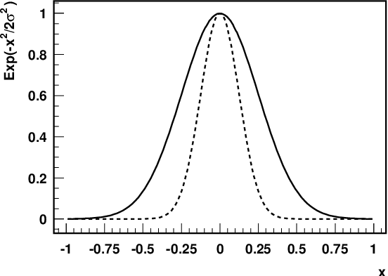
To numerically solve the evolution equations in Eqs. (107) to (110), we choose the following input correlation functions at GeV. For the quark-gluon correlation function , we choose the Fit. II of the quark-gluon correlation function from Ref. [33]. For the tri-gluon correlation functions, we choose the model introduced in Ref. [28],
| (117) |
with GeV at GeV and CTEQ6L unpolarized gluon distribution [50]. As an approximation, we also set and for less parameters since they have vanishing diagonal contribution and the size of the off-diagonal part could be smaller than that of set one correlation functions. For a better convergence of the numerical solution, we use the linear combination of the two tri-gluon correlation functions, , when we solve for the evolution equations.


We first solve the flavor non-singlet evolution equation for the quark-gluon correlation function in Eq. (99) to test the relative role of the normal DGLAP evolution term that is proportional to and the new piece that depends on the off-diagonal correlation function. In Fig. 12, we plot the twist-3 up-quark-gluon correlation as a function of at the factorization scale GeV (left) and GeV (right). The difference between the left figure and the one on the right indicates the evolution of the twist-3 correlation functions. The factorization scale dependence is a solution of the flavor non-singlet evolution equation in Eq. (99). Solid and dotted curves correspond to two different choices of the width for the off-diagonal input correlation function at and 1/8, respectively. The dashed curve is obtained by keeping only the DGLAP evolution kernel when we solve the flavor non-singlet evolution equation in Eq. (99). Similarly, we plot the twist-3 down-quark-gluon correlation as a function of at the factorization scale GeV (left) and GeV (right) in Fig. 13. Unlike the up-quark-gluon correlation function , the down-quark-gluon correlation function is negative [8]. Figures 12 and 13 clearly show that the scale dependence of the diagonal twist-3 quark-gluon correlation function does follow the evolution of the unpolarized quark distribution. The difference between the solid and the dashed curves indicates that the effect of non-DGLAP type contribution from the off-diagonal correlation function could be very important at small if the width of the off-diagonal correlation function is large.


In Figs. 14 and 15, we plot the twist-3 up-quark-gluon and down-quark-gluon correlation functions, and , as a function of at GeV (left) and GeV (right). Only difference between the solid and dotted curves in these figures and those in Figs. 12 and 13 is that we use the full set of evolution equations in Eq. (107) through (110) to solve for the factorization scale dependence of these correlation functions. The dashed curves represent the quark-gluon correlation functions obtained from the parametrization of Fit II in Ref. [33] by assuming all quark-gluon and tri-gluon correlation functions obey the DGLAP evolution. We find that non-DGLAP terms in the full evolution equations for the diagonal twist-3 correlation functions play a significant role in modifying the evolution of these correlation functions at small , where the role of the off-diagonal correlation functions is enhanced due to a larger available phase space for the evolution kernels. The extra enhancement of the solid and dotted curves over the dashed curves in Figs. 14 and 15 is mainly from the term proportional to the sum of both tri-gluon correlation functions and that we assumed to have the same sign.


In Figs. 16 and 17, we plot the twist-3 tri-gluon correlation functions, and , as a function of at GeV (left) and GeV (right), respectively. Solid and dotted curves are from solving the full evolution equations with the input correlation functions evaluated at and 1/8, respectively. Dashed curves are given by the normal CTEQ6L gluon distribution multiplied by the normalization constant (or ), which corresponds to making an assumption that all twist-3 correlation functions obey the DGLAP evolution, like the normal unpolarized PDFs. We notice that for the evolution of tri-gluon correlation functions, the difference in color factor for the DGLAP-type terms in the full evolution equations tends to compensate the contribution from the terms proportional to the off-diagonal correlation functions, so that the evolution of the tri-gluon correlation functions follow more closely to the DGLAP evolution as shown in Figs. 16 and 17.
We complete this section by stressing that the scale dependence presented in this section is sensitive to our assumption to neglect the role of the second set of twist-3 correlation functions and our model for the input tri-gluon correlation functions (equal and positive at the input scale). Although the overall features found here should be valid, the precise numerical values of these correlation functions should be extracted from a consistent global QCD analysis by comparing experimental data on SSAs and corresponding theoretical calculations, like what have been done to test the leading power QCD factorization formalism [5, 6]. The new evolution equation derived in this paper is the necessary step to make such a consistent global QCD analysis possible for twist-3 correlation functions relevant to SSAs.
VI Summary and Conclusions
We constructed two sets of twist-3 correlation functions that are responsible for generating the SSAs in the QCD collinear factorization approach. These correlation functions do not contribute to the long-distance correlation functions extracted from any measurement of parity conserving double-spin asymmetries, such as the DIS structure function . We introduced the Feynman diagram representation for the twist-3 quark-gluon and tri-gluon correlation functions and derived the cutvertices to connect the hadronic matrix elements of these correlation functions to the forward scattering Feynman diagrams. In terms of the Feynman diagram representation, we derived for the first time a closed set of evolution equations in Eqs. (86) and (89) for these quark-gluon and tri-gluon correlation functions. We also provide the explicit prescription for calculating the corresponding evolution kernels.
We calculated in the light-cone gauge the order of evolution kernels for the scale dependence of the diagonal quark-gluon and tri-gluon correlation functions that are responsible for the leading gluonic pole contribution to the SSAs. We also provided in this paper the cut vertices and corresponding projection operators necessary for performing the calculation of evolution kernels in a covariant gauge. A covariant gauge calculation requires additional Feynman diagrams that have eikonal lines connecting quark and gluon lines at the cut vertices. These additional diagrams are from the expansion of the gauge links in the matrix element definition of the twist-3 correlation functions [8]. Our calculation explicitly shows that all evolution kernels are infrared safe as they should be. In addition, we also examined infrared behavior of the evolution kernels that are more relevant to the fermionic pole contribution to the SSAs and found that these kernels are also infrared safe. We leave the details on the scale dependence of more general off-diagonal twist-3 correlation functions to a future publication.
We found that the evolution equations for the scale dependence of the diagonal twsit-3 correlation functions do not form a closed set of differential equations. The variation of the diagonal correlation functions gets contribution from the off-diagonal correlation functions. At the order of , all contributions to the evolution kernels from the diagonal correlation functions are proportional to corresponding DGLAP evolution kernels of unpolarized PDFs. In order to test the role of the off-diagonal correlation functions to the scale dependence of the diagonal correlation functions, we introduced a model for the off-diagonal correlation functions in Eq. (114) in terms of the diagonal functions plus a correlation factor characterized by a parameter . With our model, we were able to solve the evolution equations and derive the scale dependence of the diagonal twist-3 correlation functions, and test the relative strength of different sources of contribution to the scale dependence. We found within a reasonable parameter space of our model that the scale dependence of the diagonal twist-3 quark-gluon and tri-gluon correlation functions follows closely the DGLAP evolution of unpolarized PDFs, and the contribution from the off-diagonal correlation functions becomes more significant at small .
Although our observations are dependent of the model for the off-diagonal correlation functions, we believe that the overall feature found here should be valid. The precise behavior of these twist-3 correlation functions should be extracted from a consistent global QCD analysis, just like what have been done for the leading power QCD dynamics and the scale dependence of the universal PDFs [5, 6]. The evolution equations derived in this paper enable us to evaluate the NLO corrections to the SSAs systematically, which represents a necessary step moving toward the goal of global analysis of QCD dynamics beyond what have been explored by the very successful leading power QCD collinear factorization formalism. With such a global analysis, we will be able to explore the rich field of quantum correlation of multiple fields inside a polarized hadron.
Acknowledgments
We thank G. Sterman, W. Vogelsang and F. Yuan for helpful discussion. We also thank A. Belitsky and P. Ratcliffe for correspondence on references of evolution equations of twist-3 correlation functions. J.Q. thanks the Institute of High Energy Physics, Chinese Academy of Science for its hospitality during the completion of this work. This work was supported in part by the U. S. Department of Energy under Grant No. DE-FG02-87ER40371.
References
- [1] D. L. Adams et al. [E581 and E704 Collaborations], Phys. Lett. B 261, 201 (1991); D. L. Adams et al. [FNAp-E704 Collaboration], Phys. Lett. B 264, 462 (1991); K. Krueger et al., Phys. Lett. B 459, 412 (1999).
- [2] A. Bravar [Spin Muon Collaboration], Nucl. Phys. A 666, 314 (2000); A. Airapetian et al. [HERMES Collaboration], Phys. Rev. Lett. 84, 4047 (2000); Phys. Rev. D 64, 097101 (2001); Phys. Rev. Lett. 94, 012002 (2005) [arXiv:hep-ex/0408013]; V. Y. Alexakhin et al. [COMPASS Collaboration], Phys. Rev. Lett. 94, 202002 (2005) [arXiv:hep-ex/0503002]; E. S. Ageev et al. [COMPASS Collaboration], Nucl. Phys. B 765, 31 (2007) [arXiv:hep-ex/0610068]; M. Alekseev et al. [COMPASS Collaboration], arXiv:0802.2160 [hep-ex]; S. Levorato [COMPASS Collaboration], talk presented at “Second International Workshop on Transverse Polarisation Phenomena in Hard Processes (Transversity 2008)”, May 2008, Ferrara, Italy; H. Avakian, P. E. Bosted, V. Burkert and L. Elouadrhiri [CLAS Collaboration], AIP Conf. Proc. 792, 945 (2005) [arXiv:nucp-ex/0509032].
- [3] J. Adams et al. [STAR Collaboration], Phys. Rev. Lett. 92, 171801 (2004) [arXiv:hep-ex/0310058]; B. I. Abelev et al. [STAR Collaboration], Phys. Rev. Lett. 99, 142003 (2007) [arXiv:0705.4629 [hep-ex]]; arXiv:0801.2990 [hep-ex]; S. S. Adler et al. [PHENIX Collaboration], Phys. Rev. Lett. 95, 202001 (2005) [arXiv:hep-ex/0507073]; M Chiu [PHENIX Collaboration], talk presented at “The 18th International Symposium on Spin Physics (Spin 2008)”, Charlottesville, Virginia, Oct. 2008; I. Arsene et al. [BRAHMS Collaboration], Phys. Rev. Lett. 101, 042001 (2008) [arXiv:0801.1078 [nucp-ex]].
- [4] J. C. Collins, D. E. Soper and G. Sterman, Adv. Ser. Direct. High Energy Phys. 5, 1 (1988) [arXiv:hep-ph/0409313], and references therein.
- [5] J. Pumplin, D. R. Stump, J. Huston, H. L. Lai, P. Nadolsky and W. K. Tung, JHEP 0207, 012 (2002) [arXiv:hep-ph/0201195]; P. M. Nadolsky et al., Phys. Rev. D 78, 013004 (2008) [arXiv:0802.0007 [hep-ph]], and references therein.
- [6] A. D. Martin, R. G. Roberts, W. J. Stirling and R. S. Thorne, Eur. Phys. J. C 23, 73 (2002) [arXiv:hep-ph/0110215]; A. D. Martin, W. J. Stirling, R. S. Thorne and G. Watt, Phys. Lett. B 652, 292 (2007) [arXiv:0706.0459 [hep-ph]], and references therein.
- [7] A. V. Efremov and O. V. Teryaev, Sov. J. Nucl. Phys. 36, 140 (1982) [Yad. Fiz. 36, 242 (1982)]; A. V. Efremov and O. V. Teryaev, Phys. Lett. B 150, 383 (1985).
- [8] J. W. Qiu and G. Sterman, Phys. Rev. Lett. 67, 2264 (1991); Nucl. Phys. B 378, 52 (1992).
- [9] J. W. Qiu and G. Sterman, AIP Conf. Proc. 223, 249 (1991); Nucl. Phys. B 353, 137 (1991).
- [10] J. W. Qiu and G. Sterman, Phys. Rev. D 59, 014004 (1998).
- [11] H. Eguchi, Y. Koike and K. Tanaka, Nucl. Phys. B 752, 1 (2006) [arXiv:hep-ph/0604003]; Nucl. Phys. B 763, 198 (2007) [arXiv:hep-ph/0610314]; Y. Koike and K. Tanaka, Phys. Lett. B 646, 232 (2007) [Erratum-ibid. B 668, 458 (2008)] [arXiv:hep-ph/0612117]; Phys. Rev. D 76, 011502 (2007) [arXiv:hep-ph/0703169].
- [12] D. W. Sivers, Phys. Rev. D 41, 83 (1990); Phys. Rev. D 43, 261 (1991).
- [13] S. J. Brodsky, D. S. Hwang and I. Schmidt, Phys. Lett. B 530, 99 (2002) [arXiv:hep-ph/0201296]; Nucl. Phys. B 642, 344 (2002) [arXiv:hep-ph/0206259].
- [14] P. J. Mulders and R. D. Tangerman, Nucl. Phys. B 461, 197 (1996) [Erratum-ibid. B 484, 538 (1997)] [arXiv:hep-ph/9510301]; D. Boer and P. J. Mulders, Phys. Rev. D 57, 5780 (1998) [arXiv:hep-ph/9711485]; A. Bacchetta, M. Diehl, K. Goeke, A. Metz, P. J. Mulders and M. Schlegel, JHEP 0702, 093 (2007) [arXiv:hep-ph/0611265].
- [15] J. C. Collins, Phys. Lett. B 536, 43 (2002) [arXiv:hep-ph/0204004]; A. V. Belitsky, X. Ji and F. Yuan, Nucl. Phys. B 656, 165 (2003) [arXiv:hep-ph/0208038]; X. Ji, J. P. Ma and F. Yuan, Phys. Rev. D 71, 034005 (2005) [arXiv:hep-ph/0404183]; Phys. Lett. B 597, 299 (2004) [arXiv:hep-ph/0405085].
- [16] D. Boer, P. J. Mulders and F. Pijlman, Nucl. Phys. B 667, 201 (2003) [arXiv:hep-ph/0303034].
- [17] X. Ji, J. W. Qiu, W. Vogelsang and F. Yuan, Phys. Rev. Lett. 97, 082002 (2006) [arXiv:hep-ph/0602239], Phys. Rev. D 73, 094017 (2006) [arXiv:hep-ph/0604023], Phys. Lett. B 638, 178 (2006) [arXiv:hep-ph/0604128]; Y. Koike, W. Vogelsang and F. Yuan, Phys. Lett. B 659, 878 (2008) [arXiv:0711.0636 [hep-ph]].
- [18] Y. Kanazawa and Y. Koike, Phys. Lett. B 478, 121 (2000) [arXiv:hep-ph/0001021]; Phys. Rev. D 64, 034019 (2001) [arXiv:hep-ph/0012225];
- [19] A. Bacchetta, C. J. Bomhof, P. J. Mulders and F. Pijlman, Phys. Rev. D 72, 034030 (2005) [arXiv:hep-ph/0505268]; C. J. Bomhof, P. J. Mulders and F. Pijlman, Eur. Phys. J. C 47, 147 (2006) [arXiv:hep-ph/0601171].
- [20] D. Boer and W. Vogelsang, Phys. Rev. D 69, 094025 (2004) [arXiv:hep-ph/0312320];
- [21] W. Vogelsang and F. Yuan, Phys. Rev. D 72, 054028 (2005) [arXiv:hep-ph/0507266].
- [22] J. W. Qiu, W. Vogelsang and F. Yuan, Phys. Lett. B 650, 373 (2007) [arXiv:0704.1153 [hep-ph]]; Phys. Rev. D 76, 074029 (2007) [arXiv:0706.1196 [hep-ph]].
- [23] C. J. Bomhof, P. J. Mulders, W. Vogelsang and F. Yuan, Phys. Rev. D 75, 074019 (2007) [arXiv:hep-ph/0701277].
- [24] A. Bacchetta, C. Bomhof, U. D’Alesio, P. J. Mulders and F. Murgia, Phys. Rev. Lett. 99, 212002 (2007) [arXiv:hep-ph/0703153].
- [25] M. Anselmino, M. Boglione and F. Murgia, Phys. Lett. B 362, 164 (1995) [arXiv:hep-ph/9503290]; U. D’Alesio and F. Murgia, Phys. Rev. D 70, 074009 (2004) [arXiv:hep-ph/0408092]; M. Anselmino, M. Boglione, U. D’Alesio, E. Leader, S. Melis and F. Murgia, Phys. Rev. D 73, 014020 (2006) [arXiv:hep-ph/0509035].
- [26] M. Anselmino, et al., Phys. Rev. D 72, 094007 (2005) [Erratum-ibid. D 72, 099903 (2005)] [arXiv:hep-ph/0507181];
- [27] X. D. Ji, Phys. Lett. B 289, 137 (1992).
- [28] Z. B. Kang and J. W. Qiu, Phys. Rev. D 78, 034005 (2008) [arXiv:0806.1970 [hep-ph]]; Z. B. Kang, J. W. Qiu, W. Vogelsang and F. Yuan, Phys. Rev. D (in press) [arXiv:0810.3333 [hep-ph]].
- [29] F. Yuan and J. Zhou, Phys. Lett. B 668, 216 (2008) [arXiv:0806.1932 [hep-ph]].
- [30] M. Anselmino, M. Boglione, U. D’Alesio, E. Leader and F. Murgia, Phys. Rev. D 70, 074025 (2004) [arXiv:hep-ph/0407100].
- [31] P. J. Mulders and J. Rodrigues, Phys. Rev. D 63, 094021 (2001) [arXiv:hep-ph/0009343].
- [32] C. J. Bomhof and P. J. Mulders, JHEP 0702, 029 (2007) [arXiv:hep-ph/0609206]; Nucl. Phys. B 795, 409 (2008) [arXiv:0709.1390 [hep-ph]].
- [33] C. Kouvaris, J. W. Qiu, W. Vogelsang and F. Yuan, Phys. Rev. D 74, 114013 (2006) [arXiv:hep-ph/0609238].
- [34] M. Anselmino et al., arXiv:0805.2677 [hep-ph], and references therein.
- [35] see, for example: A. P. Bukhvostov, E. A. Kuraev and L. N. Lipatov, Sov. J. Nucl. Phys. 38, 263 (1983); A. P. Bukhvostov, G. V. Frolov, L. N. Lipatov and E. A. Kuraev, Nucl. Phys. B 258, 601 (1985); P. G. Ratcliffe, Nucl. Phys. B 264, 493 (1986); I. I. Balitsky and V. M. Braun, Nucl. Phys. B 311, 541 (1989); X. D. Ji and C. h. Chou, Phys. Rev. D 42, 3637 (1990); J. Kodaira, Y. Yasui, K. Tanaka and T. Uematsu, Phys. Lett. B 387, 855 (1996) [arXiv:hep-ph/9603377]; S. E. Derkachov, G. P. Korchemsky and A. N. Manashov, Nucl. Phys. B 566, 203 (2000) [arXiv:hep-ph/9909539]; V. M. Braun, G. P. Korchemsky and A. N. Manashov, Nucl. Phys. B 603, 69 (2001) [arXiv:hep-ph/0102313], and references therein.
- [36] see, for example: V. M. Braun, S. E. Derkachov and A. N. Manashov, Phys. Rev. Lett. 81, 2020 (1998) [arXiv:hep-ph/9805225]; A. Ali, V. M. Braun and G. Hiller, Phys. Lett. B266, 117 (1991); A. V. Belitsky, Nucl. Phys. B 558, 259 (1999) [arXiv:hep-ph/9903512]; A. V. Belitsky, Nucl. Phys. B 574, 407 (2000) [arXiv:hep-ph/9907420]; A. V. Belitsky, V. M. Braun, A. S. Gorsky and G. P. Korchemsky, Int. J. Mod. Phys. A 19, 4715 (2004) [arXiv:hep-th/0407232], and references therein.
- [37] see, for example: I. I. Balitsky, V. M. Braun, Y. Koike and K. Tanaka, Phys. Rev. Lett. 77, 3078 (1996) [arXiv:hep-ph/9605439]; A. V. Belitsky and D. Mueller, Nucl. Phys. B 503, 279 (1997) [arXiv:hep-ph/9702354]; A. V. Belitsky, Phys. Lett. B 453, 59 (1999) [arXiv:hep-ph/9902361], and references therein.
- [38] A. A. Henneman, D. Boer and P. J. Mulders, Nucl. Phys. B 620, 331 (2002) [arXiv:hep-ph/0104271].
- [39] J. C. Collins and J. W. Qiu, Phys. Rev. D 39, 1398 (1989).
- [40] A. H. Mueller, Phys. Rept. 73, 237 (1981).
- [41] R. K. Ellis, W. Furmanski and R. Petronzio, Nucl. Phys. B 212, 29 (1983).
- [42] J. W. Qiu, Phys. Rev. D 42, 30 (1990).
- [43] R. Brock et al. [CTEQ Collaboration], Rev. Mod. Phys. 67, 157 (1995).
- [44] G. Sterman, Lectures given at Theoretical Advanced Study Institute in Elementary Particle Physics (TASI 95): QCD and Beyond, Boulder, CO, 4-30 Jun 1995. Published in Boulder TASI 95:327-408 [arXiv:hep-ph/9606312].
- [45] Yu. Dokshitzer, Sov. Phys. JETP 46, 1649 (1977); V. N. Gribov and L. N. Lipatov, Sov. Nucl. Phys. 15, 438 (1972); 15, 675 (1972); G. Alteralli and G. Parisi, Nucl. Phys. B 126, 298 (1977).
- [46] W. Vogelsang and F. Yuan, talk given by Vogelsang at The 18th International Symposium on Spin Physics (Spin 2008), Charlottesville, VA, 6-11 October 2008.
- [47] R. L. Jaffe, Nucl. Phys. B 229, 205 (1983).
- [48] M. Luo, J. W. Qiu and G. Sterman, Phys. Rev. D 49, 4493 (1994).
- [49] V. Barone, A. Drago and P. G. Ratcliffe, Phys. Rept. 359, 1 (2002) [arXiv:hep-ph/0104283]; X. Artru and M. Mekhfi, Z. Phys. C 45, 669 (1990); J. C. Collins, Nucl. Phys. B 396, 161 (1993) [arXiv:hep-ph/9208213].
- [50] J. Pumplin, D. R. Stump, J. Huston, H. L. Lai, P. Nadolsky and W. K. Tung, JHEP 0207, 012 (2002) [arXiv:hep-ph/0201195].