跳到论文正文
W Papers独立论文阅读器 arXiv:0811.3080 论文正文 计算阅读时间 · 0%
引用这篇论文根据当前论文元数据生成,正式投稿前建议核对。


License: arXiv.org perpetual non-exclusive license
arXiv:0811.3080v1 [cond-mat.stat-mech] 19 Nov 2008

Factorization of percolation density correlation functions for clusters touching the sides of a rectangle

J. J. H. Simmons Email: j.simmons1@physics.ox.ac.uk Affiliation: Rudolf Peierls Centre for Theoretical Physics, 1 Keble Road, Oxford OX1 3NP, UK    Robert M. Ziff Email: rziff@engin.umich.edu Affiliation: Michigan Center for Theoretical Physics and Department of Chemical Engineering, University of Michigan, Ann Arbor MI 48109-2136    Peter Kleban Email: kleban@maine.edu Affiliation: LASST and Department of Physics & Astronomy, University of Maine, Orono, ME 04469, USA
August 24, 2026
Abstract

In this paper we consider the density, at a point z=x+i​yz=x+iy, of critical percolation clusters that touch the left (PL​(z)P_{L}(z)), right (PR​(z)P_{R}(z)), or both (PL​R​(z)P_{LR}(z)) sides of a rectangular system, with open boundary conditions on the top and bottom sides. While each of these quantities is nonuniversal and indeed vanishes in the continuum limit, the ratio C⁡(z)=PL​R​(z)/PL​(z)​PR​(z)​ΠhC(z)=P_{LR}(z)/\sqrt{P_{L}(z)P_{R}(z)\Pi_{h}}, where Πh\Pi_{h} is the probability of left-right crossing given by Cardy, is a universal function of zz. With wired (fixed) boundary conditions on the left- and right-hand sides, high-precision numerical simulations and theoretical arguments show that C⁡(z)C(z) goes to a constant C0=27/2 3−3/4π5/2Γ(1/3)−9/2=1.0299268…C_{0}=2^{7/2}\;3^{-3/4}\,\pi^{5/2}\;\Gamma(1/3)^{-9/2}=1.0299268\ldots for points far from the ends, and varies by no more than a few percent for all zz values. Thus PL​R​(z)P_{LR}(z) factorizes over the entire rectangle to very good approximation. In addition, the numerical observation that C⁡(z)C(z) depends upon xx but not upon yy leads to an explicit expression for C⁡(z)C(z) via conformal field theory for a long rectangle (semi-infinite strip). We also derive explict expressions for PL​(z)P_{L}(z), PR​(z)P_{R}(z), and PL​R​(z)P_{LR}(z) in this geometry, first by assuming yy-independence and then by a full analysis that obtains these quantities exactly with no assumption on the yy behavior. In this geometry we obtain, in addition, the corresponding quantities in the case of open boundary conditions, which allows us to calculate C⁡(z)C(z) in the open system. We give some theoretical results for an arbitrary rectangle as well. Our results also enable calculation of the finite-size corrections to the factorization near an isolated anchor point, for the case of clusters anchored at points. Finally, we present numerical results for a rectangle with periodic b.c. in the horizontal direction, and find C⁡(z)C(z) approaches a constant value C1≈1.022C_{1}\approx 1.022.

Keywords: 
percolation, correlation functions, factorization, conformal field theory, numerical simulation

I Introduction

Percolation at the critical point has many well-known universal properties, including universal critical exponents, scaling functions, and amplitude ratios. Universality means that the properties are the same for all realizations of the system (with a given dimensionality) in the continuum or field-theory limit. Crossing probabilities are also universal and have received a great deal of attention since the work of Cardy [1] and Langlands et al. [2], and renewed interest more recently with the development of Schramm-Loewner Evolution (SLE) [3] and a new set of results for percolation [4].

A more detailed picture of the critical system can be obtained by examining the correlations within clusters of connected sites. In previous work [5, 6], we demonstrated, by use of conformal field theory and high-precision simulation, certain exact and universal factorizations of higher-order correlation functions in terms of lower-order correlation functions for percolation clusters in two dimensions at the percolation point. In that work, the correlation functions involved the density of critical percolation clusters constrained to touch one or two isolated boundary points, or single boundary intervals. Here we extend those results by considering densities constrained to touch one or two distinct boundary intervals, which is a more difficult problem.

Specifically, we consider the quantities PL​(z)P_{L}(z), PR​(z)P_{R}(z), and PL​R​(z)P_{LR}(z), which give the density of percolation clusters at a point z=x+i​yz=x+iy that touch the left, right, or both sides of a rectangle, respectively, as well as Πh\Pi_{h} the probability of a horizontal crossing (i.e., one or more clusters that touch both left and right sides) which is given by Cardy’s formula [1]. PL​(z)P_{L}(z), PR​(z)P_{R}(z), and PL​R​(z)P_{LR}(z) also determine the probabilities that the given boundaries are connected to zz, or more precisely to a disk of radius ε\varepsilon around zz. Individually they are non-universal and furthermore go to zero as the lattice mesh size (or ε\varepsilon) goes to zero. However, we find numerically and prove via conformal field theory that the ratio

C⁡(z)=PL​R​(z)PL​(z)​PR​(z)​Πh,C(z)=\frac{P_{LR}(z)}{\sqrt{P_{L}(z)P_{R}(z)\Pi_{h}}}\;, (1)

is a universal function of zz in the limit that ε\varepsilon goes to zero, depending only upon the boundary conditions on the sides of the rectangle.

For most of this paper (except the last section) the boundary conditions (b.c) are assumed to be open, or free, on the top and bottom sides, and either open or wired on the left and right sides. The behavior of C⁡(z)C(z) near the left and right sides depends strongly on our choice of b.c. However, for rectangles with width WW greater than a few times their height HH, C⁡(z)C(z) goes exponentially to a universal constant, C0C_{0}, for points that are on the order of WW away from the left and right sides, regardless of the boundary conditions on those sides. We find that the asymptotic value C0C_{0} is the same as that found for the case of point anchors [5, 6]:

C0=27/2​π5/233/4​Γ​(1/3)9/2=1.0299268​….C_{0}=\frac{2^{7/2}\;\pi^{5/2}}{3^{3/4}\;\Gamma(1/3)^{9/2}}=1.0299268\ldots\;. (2)

This agreement is expected because for points zz far from either vertical side the difference between anchoring to boundary points or small intervals becomes negligible.

Furthermore, we find the surprising result that with wired boundary conditions on the left- and right-hand sides C⁡(z)C(z) depends only upon the horizontal coordinate xx and not on yy, even though the individual functions PL​(z)P_{L}(z) etc. have a strong dependence on yy. With wired boundary conditions all clusters touching the boundary are assumed to be connected together, so that if there is a crossing cluster all other clusters touching either boundary are also part of it. For this boundary condition, C⁡(z)C(z) goes to 1 as zz approaches the left or right sides, and remains within a few percent of 11 for all zz, so that factorization is a good approximation everywhere in the rectangle.

The results simplify particularly nicely for the case of a long rectangular system which we approximate as a semi-infinite strip (of unit width). In that case, we find

C⁡(x)\displaystyle C(x) =\displaystyle= C0​2F1(−1/2,−1/3,7/6,e−2​π​x)2F1(−1/2,−2/3,5/6,e−2​π​x)\displaystyle C_{0}\frac{{}_{2}F_{1}(-1/2,-1/3,7/6,e^{-2\pi x})}{\sqrt{{}_{2}F_{1}(-1/2,-2/3,5/6,e^{-2\pi x})}} (3)
∼\displaystyle\sim C0​(1−235​e−2​π​x+83425025​e−4​π​x+…)(for x→∞)\displaystyle C_{0}\left(1-\frac{2}{35}e^{-2\pi x}+\frac{834}{25025}e^{-4\pi x}+\ldots\right)\qquad\hbox{(for $x\to\infty$)}

where xx is the distance from one end. We also provide numerical confirmation of this result.

Refer to caption
Figure 1: Plots of PL​(z)P_{L}(z) (top), PL​R​(z)P_{LR}(z) (center), and C⁡(z)C(z) (bottom) for a 127×255127\times 255 system with wired b.c. on the left and right-hand sides.

If we consider open boundary conditions on the left- and right-hand sides, then C⁡(z)C(z) remains universal and approaches C0C_{0} far from the vertical sides. However, near the left- and right-hand sides, C⁡(z)C(z) depends upon both xx and yy. Furthermore, when zz approaches the left or right side C⁡(z)C(z) goes to zero, so the factorization breaks down.

We have also simulated C⁡(z)C(z) with periodic boundary conditions on the horizontal sides. Here, of course, all PP’s are trivially independent of yy and therefore C⁡(z)C(z) is again a function of xx only (for either open or wired b.c. on the vertical sides). C⁡(z)C(z) goes to a constant value different from C0C_{0}, viz. C1≈1.022​…C_{1}\approx 1.022\dots at points far from the ends of the cylinder. We do not have a theoretical prediction for this value.

Section II gives our numerical results which show approximate factorization and interesting y−y-dependence with wired b.c. , and section III presents our theoretical derivation of those results; first for the case of the semi-infinite strip (including open b.c. results and complete expressions for the densities) and then for the complete rectangle. We compare these predictions with further numerical results. In section IV we consider the problem of finite-size corrections around an anchoring point. We show that our formulas for wired b.c. predict these corrections. In section V we present our numerical results for periodic b.c., and section VI gives our conclusions. The appendix presents a full derivation of the semi-infinite strip densities, which confirms that our expressions for PL​(z)P_{L}(z), PR​(z)P_{R}(z), and PL​R​(z)P_{LR}(z) are exact, as is the y−y-independence of C⁡(z)C(z) with wired b.c. .

II Numerical results for C(z)

To investigate the probabilities PL​(z)P_{L}(z), etc., we carried out simulations in rectangular systems of dimensions 63×12763\times 127, and 127×255127\times 255. (The arrays used in the computer code were actually exact powers of two, but one column and row were left open, along with periodic b.c., to efficiently simulate the open boundaries.) We used a square lattice and considered both bond and site percolation at the critical thresholds 1/21/2 and 0.59274600.5927460 [7, 8, 9] respectively. The random-number generator used was R(471,1586,6988,9689) given in [10]. We kept track of the average density of clusters that touched the left, right, and both sides of the rectangular systems, where the density at a point is simply the number of times a cluster touching the desired boundary or boundaries includes that point, divided by the total number of trials. In Fig. 1 we show plots of the densities for bond percolation on a lattice of size 127×255127\times 255 sites with wired boundary conditions on the left and right-hand sides. The top figure shows PL​(z)P_{L}(z); the plot of PR​(z)P_{R}(z) is identical but flipped horizontally. Along the left and right-hand boundaries PL​(z)P_{L}(z) is constant and equal to 11 and Πh\Pi_{h} respectively, both a consequence of the wired b.c. In the intermediate region there is an exponential drop-off in the density.

In the center plot in Fig. 1 we show PL​R​(z)P_{LR}(z), which is roughly independent of xx away from the ends. The lower figure shows C⁡(z)C(z) defined by Eq. (1), and here one can see the striking result that C⁡(z)C(z) depends upon the xx-coordinate but appears to be independent of yy, in spite of the strong yy-dependence of the functions that define it. Note that the range of the vertical scale now goes from 11 to 1.031.03.

At the two wired boundaries x=0x=0 and x=wx=w, C⁡(z)C(z) goes to 1. For bond percolation, where all sites are effectively occupied while the bonds are diluted (occupied with probability pp), C⁡(z)C(z) is identically 1 at these two boundaries because PL​(z)→1P_{L}(z)\to 1, PL​R​(z)→ΠhP_{LR}(z)\to\Pi_{h}, and PR​(z)→ΠhP_{R}(z)\to\Pi_{h} as x→0x\to 0 for a given yy (and similarly for x→wx\to w). For site percolation, where sites including those in the first and last columns are occupied with probability p=0.592746​…p=0.592746\ldots, we have PL​(z)→pP_{L}(z)\to p, PL​R​(z)→p​ΠhP_{LR}(z)\to p\Pi_{h}, and PR​(z)→p​ΠhP_{R}(z)\to p\Pi_{h} as x→0x\to 0 for a given yy, so here C⁡(z)→1C(z)\to 1 but only on the average, not identically as in the bond case, and there are small fluctuations. We do not show the plots for site percolation as they are quite similar to those for bond percolation.

Away from the left- and right-hand boundaries, C⁡(z)C(z) approaches the value C0C_{0} given in Eq. (2). The quantity C0C_{0} first appeared the context of the densities of clusters touching one or two boundary anchor points, where after just several lattice spacings away from the anchors the analogous C⁡(z)C(z) was found to go to C0C_{0} everywhere [5]. The reason that the same constant appears here is that, from a distance, the interval looks like a point. Furthermore, as discussed in more detail below, a conformal transformation converts the interval problem to the point anchor problem, and shows that indeed C⁡(z)C(z) far from the vertical boundaries of the rectangle asymptotes to C0C_{0}.

Refer to caption
Figure 2: Plot of PL​(z)/PL​R​(z)P_{L}(z)/P_{LR}(z) for the wired 127×255127\times 255 system of Fig. 1.

Fig. 2 shows a plot of the ratio PL​(z)/PL​R​(z)P_{L}(z)/P_{LR}(z) for the 127×255127\times 255 system as shown in Fig. 1, showing quite clearly that this ratio is only a function of xx and not yy for wired b.c. Likewise, PL​(z)/PR​(z)P_{L}(z)/P_{R}(z) only depends on yy (this follows because C⁡(z)C(z) is only a function of yy). Thus, all three quantities PL​(z)P_{L}(z), PR​(z)P_{R}(z), and PL​R​(z)P_{LR}(z) have a common yy dependence for a given value of xx. We will use this to motivate our theoretical results.

In Fig. 3 we show similar data for a 63×12763\times 127 bond percolation system, this time plotted as contour plots. The apparent yy independence of C⁡(z)C(z) is quite clear. For much smaller system sizes (e.g. 15×3115\times 31), finite-size effects do lead to visible curvature in the contours of C⁡(z)C(z) (not shown here).

The data for x=1,…,5x=1,\ldots,5 for a system of size 127×255127\times 255 are shown in the upper plot in Fig. 4, showing the fluctuation in the data about the constant values. These rather large fluctuations are due to the fact that the probabilities PR​(z)P_{R}(z) and PL​R​(z)P_{LR}(z) are quite small for zz near the sides. Here 1.14⋅1091.14\cdot 10^{9} samples were generated, a similar number as for the other plots. The lower plot shows the same simulation with open b.c. for comparison; the dependence on b.c. is readily apparent.

Refer to caption
Figure 3: Contour plots of PL​(z)P_{L}(z) (top), PL​R​(z)P_{LR}(z) (center), and C⁡(z)C(z) (bottom) for a 63×12763\times 127 system with wired b.c. on the left and right-hand sides (similar to Fig. 1 but here as contour plots). In the plot of C⁡(z)C(z) (lower figure), the contours are at 1.0051.005, 1.0101.010, 1.0151.015, 1.0201.020, and 1.0251.025. The lower figure may be compared with Fig. 10, which shows a similar plot for open b.c.  where the behavior is quite different.
Refer to caption
Refer to caption
Figure 4: Top figure: C⁡(z)C(z) as a function of YY for X=1,2,3,4,5X=1,2,3,4,5 (bottom to top) for a system of size height×\timeswidth = 127×255127\times 255, with wired b.c. on the sides. Bottom figure: same simulation with open b.c. (Note the change of vertical scale.)

In Fig. 5 we show Copen​(z)C_{\mathrm{open}}(z) for the case of open boundary conditions on the left and right-hand sides. Here the behavior differs markedly. While Copen​(z)C_{\mathrm{open}}(z) still approaches the value C0C_{0} away from the sides, closer to them a significant yy-dependence of C⁡(z)C(z) can be seen. Also, C⁡(z)C(z) does not go to 11 at those sides as it does in the wired case, but rather drops to 00, highlighting the sensitivity of the factorization to boundary conditions.
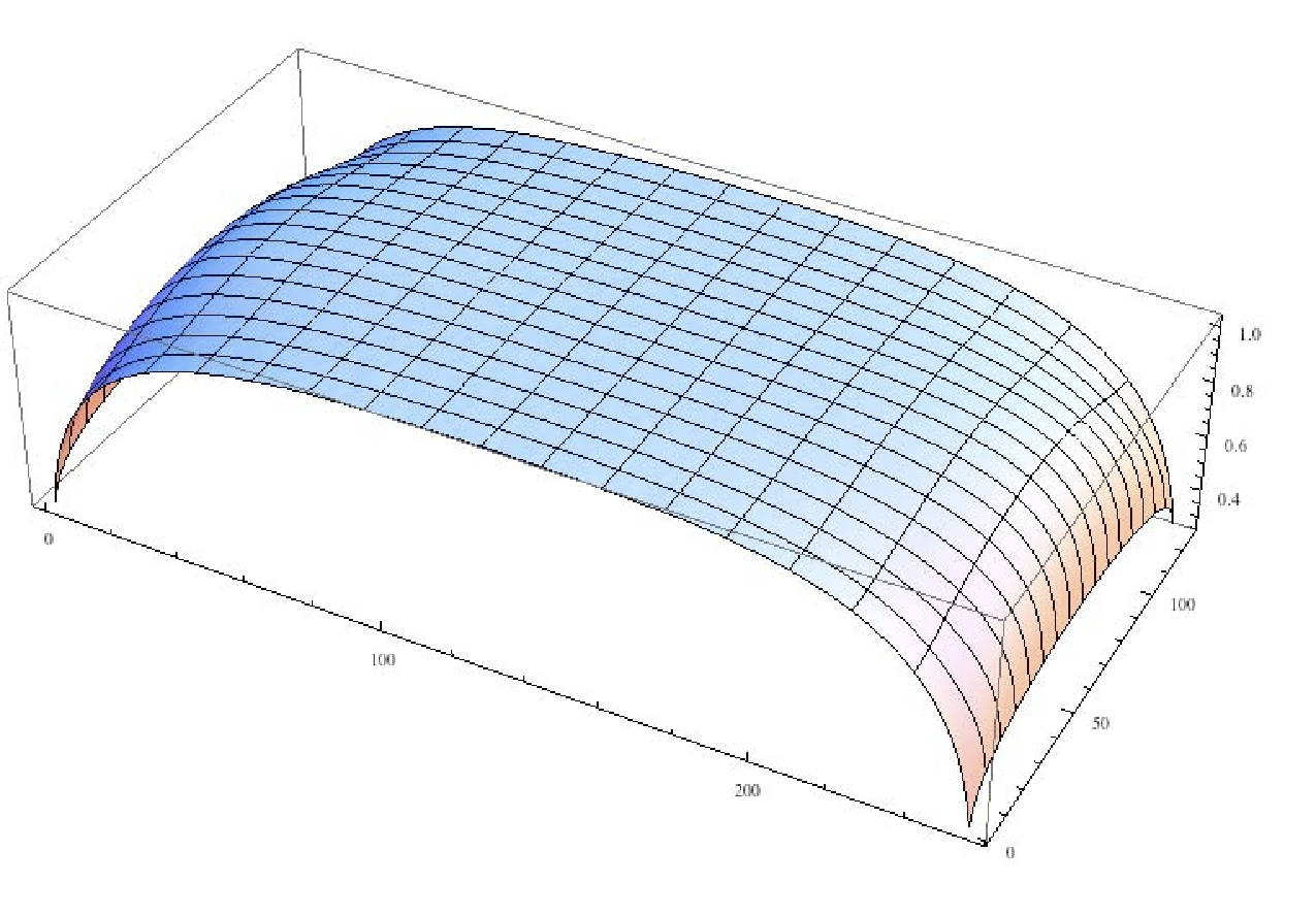
Refer to caption
Figure 5: Plot of numerical results for Copen​(z)C_{\mathrm{open}}(z) for a system of size 127×255127\times 255 with open boundaries on all sides. In contrast to the wired case, Fig 1, Copen​(z)C_{\mathrm{open}}(z) goes to a value much less than 1 at the ends, going to zero as the system size increases to infinity. The dependence of Copen​(z)C_{\mathrm{open}}(z) upon the yy coordinate is evident here.

III Theoretical results

In this section we use boundary conformal field theory to calculate C⁡(z)C(z). This quantity (see (1)) is given by a ratio of various densities. Our work in [5, 6] illustrates the method by which such densities can be derived from correlation functions in conformal field theory with c=0c=0. The three densities we are interested in arise as different conformal blocks for the same set of operators, being distinguished by fusion rules, as we will see. Thus in the upper half-plane ℍ\mathbb{H}, with w=u+i​vw=u+iv,

PL​R​(w),PL​(w),PR​(w)∼⟨ϕ1,2​(u1)​ϕ1,2​(u2)​ψ​(w3,w¯3)​ϕ1,2​(u4)​ϕ1,2​(u5)⟩,P_{LR}(w),P_{L}(w),P_{R}(w)\sim\langle\phi_{1,2}(u_{1})\phi_{1,2}(u_{2})\psi(w_{3},\bar{w}_{3})\phi_{1,2}(u_{4})\phi_{1,2}(u_{5})\rangle\;, (4)

where the boundary operator ϕ1,2​(u)\phi_{1,2}(u), with conformal dimension h1,2=0h_{1,2}=0, implements a change from open to wired (free to fixed) boundary conditions at the point uu, and the “magnetization” operator ψ​(w):=ϕ3/2,3/2​(w)\psi(w):=\phi_{3/2,3/2}(w), with conformal dimension hψ=h¯ψ=5/96h_{\psi}=\bar{h}_{\psi}=5/96, measures the density of clusters at a point ww in the upper half-plane. The other quantity of interest, Πh\Pi_{h}, is simply the probability that there exists a crossing cluster in the rectangle, given by Cardy’s formula (which itself follows from a correlation function like (4) but without the ψ\psi operator) [1].

These correlation functions can be constructed from the conformal blocks allowed by (4). However, computing these conformal blocks is a formidable task involving a six-point correlation function that depends on three independent cross-ratios. We can make the calculation tractable by exploiting the observed independence on the vertical coordinate in the rectangle: C⁡(x,y)=C⁡(x)C(x,y)=C(x). Letting y3→0y_{3}\to 0 (so v3→0v_{3}\to 0 in ℍ\mathbb{H}), the bulk magnetization operator ψ\psi in ℍ\mathbb{H} is replaced with a boundary magnetization operator, ϕ1,3​(u3)\phi_{1,3}(u_{3}) so that

PL​R​(u),PL​(u),PR​(u)∼⟨ϕ1,2​(u1)​ϕ1,2​(u2)​ϕ1,3​(u3)​ϕ1,2​(u4)​ϕ1,2​(u5)⟩.P_{LR}(u),P_{L}(u),P_{R}(u)\sim\langle\phi_{1,2}(u_{1})\phi_{1,2}(u_{2})\phi_{1,3}(u_{3})\phi_{1,2}(u_{4})\phi_{1,2}(u_{5})\rangle\;. (5)

Note that (5) is a five-point function involving only boundary operators that we will compute shortly. In this section, we assume yy-independence throughout. However, the appendix shows that our results are valid without this assumption in the case of the semi-infinite strip.

We next determine (5) in the upper half-plane, and then transform the result into the appropriate geometry. (This transformation leaves CC invariant [5].)

In subsections III.1 and III.3 we find closed expressions for PL​R​(x)P_{LR}(x), PL​(x)P_{L}(x), and PR​(x)P_{R}(x) in the semi-infinite strip and rectangle. The appendix verifies that for the case of a semi-infinite strip these expressions are valid without assuming yy-independence.

Note that the variables zz and xx represent bulk and boundary densities in the rectangle or strip while ww and uu represent bulk and boundary densities in ℍ\mathbb{H}.

III.1 Semi-infinite strip

We next consider the semi-infinite strip, which approximates the behavior near the end of a long rectangle. This is equivalent to replacing the right-hand interval with a point operator because it is vanishingly likely that two distinct clusters emanate from the distant end. Depending on which of the densities we are calculating we make use of the fusion rules to replace ϕ1,2​(u4)​ϕ1,2​(u5)\phi_{1,2}(u_{4})\phi_{1,2}(u_{5}) with either 𝟏​(∞)\mathbf{1}(\infty) or ϕ1,3​(∞)\phi_{1,3}(\infty), which significantly simplifies the calculation.

Because ϕ1,3\phi_{1,3} is the boundary magnetization operator, the fusion ϕ1,2×ϕ1,2=ϕ1,3\phi_{1,2}\times\phi_{1,2}=\phi_{1,3} conditions the wired interval to connect to other objects marked in the correlation function. For example, to calculate PR​(u)P_{R}(u) and PL​R​(u)P_{LR}(u) and then transform the result into the semi-infinite strip we insert the ϕ1,3​(∞)\phi_{1,3}(\infty) operator, because these two quantities require that a cluster connect the point at infinity with uu. (Here and in the remainder of this section we ignore the scaling factor and operator product expansion (OPE) coefficient in this fusion since they cancel in the ratios that we calculate.)

The fusion ϕ1,2×ϕ1,2=𝟏\phi_{1,2}\times\phi_{1,2}=\mathbf{1} places no condition on the connectivity of the wired interval. So we get configurations with the interval isolated and with it connected to other points. Note that the identity fusion encompasses all of the configurations in the ϕ1,3\phi_{1,3} bulk-boundary fusion as well. This mirrors Cardy’s derivation of the horizontal crossing probability, where Πh\Pi_{h} corresponds to the ϕ1,3\phi_{1,3} conformal block while the identity block counts all configurations including those with a horizontal crossing [1].

As mentioned, one can calculate PR​(u)P_{R}(u) and PL​R​(u)P_{LR}(u) using the correlation function

⟨ϕ1,2(u1)ϕ1,2(u2)ϕ1,3(u3)ϕ1,3(u4)⟩=(u4−u3)−2/3F((u2−u1)​(u4−u3)(u3−u1)​(u4−u2)).\langle\phi_{1,2}(u_{1})\phi_{1,2}(u_{2})\phi_{1,3}(u_{3})\phi_{1,3}(u_{4})\rangle=(u_{4}-u_{3})^{-2/3}F\left(\frac{(u_{2}-u_{1})(u_{4}-u_{3})}{(u_{3}-u_{1})(u_{4}-u_{2})}\right)\;. (6)

The null-state for ϕ1,2\phi_{1,2} gives

0=(1/3(u4−u1)2+1/3(u3−u1)2−∂u4u4−u1−∂u3u3−u1−∂u2u2−u1−32∂u12)⟨ϕ1,2(u1)ϕ1,2(u2)ϕ1,3(u3)ϕ1,3(u4)⟩.0=\left(\frac{1/3}{(u_{4}-u_{1})^{2}}+\frac{1/3}{(u_{3}-u_{1})^{2}}-\frac{\partial_{u_{4}}}{u_{4}-u_{1}}-\frac{\partial_{u_{3}}}{u_{3}-u_{1}}-\frac{\partial_{u_{2}}}{u_{2}-u_{1}}-\frac{3}{2}\partial_{u_{1}}^{2}\right)\langle\phi_{1,2}(u_{1})\phi_{1,2}(u_{2})\phi_{1,3}(u_{3})\phi_{1,3}(u_{4})\rangle\;. (7)

Applying (7) to (6) and using conformal symmetry to take {u1,u2,u3,u4}\{u_{1},u_{2},u_{3},u_{4}\} ⇒\Rightarrow {0,λ,1,∞}\{0,\lambda,1,\infty\} in the usual manner, so that λ\lambda is the cross-ratio, we find

0=F′′​(λ)+2​(1−2​λ)3​λ​(1−λ)​F′​(λ)−29​(1−λ)2​F​(λ).0=F^{\prime\prime}(\lambda)+\frac{2(1-2\lambda)}{3\lambda(1-\lambda)}F^{\prime}(\lambda)-\frac{2}{9(1-\lambda)^{2}}F(\lambda)\;. (8)

The solutions yield the conformal blocks

F𝟏​(λ)\displaystyle F_{\mathbf{1}}(\lambda) =\displaystyle= (1−λ)2/3​F12​(1/3,4/3,2/3,λ),and\displaystyle(1-\lambda)^{2/3}{}_{2}F_{1}(1/3,4/3,2/3,\lambda)\;,\quad\mathrm{and} (9)
Fϕ1,3​(λ)\displaystyle F_{\phi_{1,3}}(\lambda) =\displaystyle= λ1/3​(1−λ)2/3​F12​(2/3,5/3,4/3,λ).\displaystyle\lambda^{1/3}(1-\lambda)^{2/3}{}_{2}F_{1}(2/3,5/3,4/3,\lambda)\;. (10)

Here the index on the blocks represents the corresponding fusion channel of the ϕ1,2\phi_{1,2} operators.

Refer to caption
Figure 6: Schematic representation of the two types of cluster configurations consistent with ⟨ϕ1,2​(0)​ϕ1,2​(λ)​ϕ1,3​(1)​ϕ1,3​(∞)⟩\langle\phi_{1,2}(0)\phi_{1,2}(\lambda)\phi_{1,3}(1)\phi_{1,3}(\infty)\rangle, translated into the strip geometry.
Refer to caption
Figure 7: Semi-infinite strip mapping.

By the above, we may identify the configurations with (0,λ)(0,\lambda) connected to 11 and infinity with the conformal block Fϕ1,3​(λ)F_{\phi_{1,3}}(\lambda). Upon mapping into the strip this correlation will become PL​R​(x)P_{LR}(x) as illustrated in Fig. 6(a).

The conformal block F𝟏​(λ)F_{\mathbf{1}}(\lambda) represents the configurations with (0,λ)(0,\lambda) isolated from, as well as connected to, 11 and infinity. Thus upon mapping to the strip (see Fig. 7) this block becomes PR​(x)P_{R}(x), which includes all configurations with xx connected to RR, as illustrated in Fig. 6(a&b). Note that F𝟏​(λ)F_{\mathbf{1}}(\lambda) (in ℍ\mathbb{H}) includes configurations where uu and RR are not directly connected, but instead connect through the wired boundary conditions on the left side. This subtlety will be discussed in more detail in section III.2.

Having found PL​R​(u)P_{LR}(u) and PR​(u)P_{R}(u) we need only determine PL​(u)P_{L}(u). Configurations of this type don’t need to cross to the right-hand side, so instead of placing ϕ1,3\phi_{1,3} at infinity we place an identity; thus PL​(u)P_{L}(u) is proportional to a three point function.

Thus, including the proper normalizations and scaling factors we find

PL​R​(u)\displaystyle P_{LR}(u) =\displaystyle= ⟨ϕ1,2(0)ϕ1,2(λ)[1,3]ϕ1,3(1)ϕ1,3(ξ)⟩=C112C222ξ−2/3Fϕ1,3(λ),\displaystyle\langle\phi_{1,2}(0)\phi_{1,2}(\lambda)_{[1,3]}\phi_{1,3}(1)\phi_{1,3}(\xi)\rangle\quad=\quad C_{112}C_{222}\xi^{-2/3}F_{\phi_{1,3}}(\lambda)\;, (11)
PL​(u)\displaystyle P_{L}(u) =\displaystyle= ⟨ϕ1,2(0)ϕ1,2(λ)ϕ1,3(1)⟩=C112λ1/3(1−λ)−1/3,\displaystyle\langle\phi_{1,2}(0)\phi_{1,2}(\lambda)\phi_{1,3}(1)\rangle\phantom{\phi_{1,3}(\xi)_{[1,2]}}\quad=\quad C_{112}\lambda^{1/3}(1-\lambda)^{-1/3}\;, (12)
Πh\displaystyle\Pi_{h} =\displaystyle= ⟨ϕ1,2(0)ϕ1,2(λ)ϕ1,3(ξ)⟩=C112λ1/3ξ−2/3and,\displaystyle\langle\phi_{1,2}(0)\phi_{1,2}(\lambda)\phi_{1,3}(\xi)\rangle\phantom{\phi_{1,3}(1)_{[1,2]}}\quad=\quad C_{112}\lambda^{1/3}\xi^{-2/3}\;\qquad\mathrm{and}, (13)
PR​(u)\displaystyle P_{R}(u) =\displaystyle= ⟨ϕ1,2(0)ϕ1,2(λ)[1,1]ϕ1,3(1)ϕ1,3(ξ)⟩=ξ−2/3F𝟏(λ),\displaystyle\langle\phi_{1,2}(0)\phi_{1,2}(\lambda)_{[1,1]}\phi_{1,3}(1)\phi_{1,3}(\xi)\rangle\quad=\quad\xi^{-2/3}F_{\mathbf{1}}(\lambda)\;, (14)

where the variable ξ(→∞)\xi(\to\infty) indicates the order of magnitude of the length of the rectangle, the bracketed subscript notation denotes the fusion channel propagating between the operators separated (following Bauer and Bernard [11]), and the indices on the (boundary) operator product expansion coefficients Ci​j​kC_{ijk} follow the convention of [12] with index jj representing the j−j-leg boundary operator ϕ1,1+j\phi_{1,1+j}. Both operator product expansion coefficients that appear above are previously known: C112=22π3/Γ(1/3)3=0.56604668…C_{112}{}^{2}=2\pi\sqrt{3}/\Gamma(1/3)^{3}=0.56604668\ldots is most familiar as the leading coefficient in Cardy’s formula [1], while C222=C0C_{222}=C_{0} arose in the factorization formula in [5, 6]. Note that the expressions for PL​(u)P_{L}(u) and Πh\Pi_{h} could also be obtained as limiting cases of Cardy’s formula when one interval shrinks to a point.

For future reference, note that if the interval LL is not connected to either uu or RR we have

PL¯​R(u)=⟨ϕ1,3(1)ϕ1,2(λ)∂[1,2]ϕ1,2(0)ϕ1,3(ξ)⟩=K∂ϕ1,2ξ−2/3G∂ϕ1,2(λ),P_{\bar{L}R}(u)=\langle\phi_{1,3}(1)\phi_{1,2}(\lambda)_{\partial[1,2]}\phi_{1,2}(0)\phi_{1,3}(\xi)\rangle=K_{\partial\phi_{1,2}}\xi^{-2/3}G_{\partial\phi_{1,2}}(\lambda)\;, (15)

where

G∂ϕ1,2​(λ)=(1−λ)2/3​F12​(1/3,4/3,2,1−λ)andK∂ϕ1,2=8​π29​Γ​(1/3)3.G_{\partial\phi_{1,2}}(\lambda)=(1-\lambda)^{2/3}{}_{2}F_{1}(1/3,4/3,2,1-\lambda)\qquad\mathrm{and}\qquad K_{\partial\phi_{1,2}}=\frac{8\,\pi^{2}}{9\,\Gamma(1/3)^{3}}\;. (16)

This can be deduced by observing that PL¯​R​(u)=PR​(u)−PL​R​(u)P_{\bar{L}R}(u)=P_{R}(u)-P_{LR}(u) and using the crossing symmetry relation for this correlation function,

K∂ϕ1,2​G∂ϕ1,2​(λ)=F𝟏​(λ)−C112​C222​Fϕ1,3​(λ).K_{\partial\phi_{1,2}}G_{\partial\phi_{1,2}}(\lambda)=F_{\mathbf{1}}(\lambda)-C_{112}C_{222}F_{\phi_{1,3}}(\lambda)\;. (17)

In (15) we label the propagation channel and conformal block with ∂ϕ1,2\partial\phi_{1,2} in order to be consistent with the underlying logarithmic conformal field theory [4]. However, for present purposes the fusion ϕ1,3×ϕ1,2\phi_{1,3}\times\phi_{1,2} is more complicated to interpret physically than the ϕ1,2×ϕ1,2\phi_{1,2}\times\phi_{1,2} fusion discussed above, so while we include the notation for accuracy, the distinction is unimportant here and in what follows.

Combining (1) and (9)–(14) we find

C⁡(λ)=C0​1−λ​F12​(2/3,5/3,4/3,λ)F12​(1/3,4/3,2/3,λ).C(\lambda)=C_{0}\sqrt{1-\lambda}\;\frac{{}_{2}F_{1}(2/3,5/3;4/3;\lambda)}{\sqrt{{}_{2}F_{1}(1/3,4/3;2/3;\lambda)}}\;. (18)

Now map from the semi-infinite strip 𝕊={z=x+iy| 0<x, 0<y<1}\mathbb{S}=\{z=x+iy\,|\,0<x,\;0<y<1\} via

w⁡(z)=cosh2⁡(π​z/2)cosh2⁡(π​x/2),w(z)=\frac{\cosh^{2}(\pi z/2)}{\cosh^{2}(\pi x/2)}\;, (19)

which takes the point xx on the lower side of the strip to 11 in the upper half-plane (see Fig. 7).

The cross-ratio is given by

λ=w⁡(0)=sech2​(π​x/2).\lambda=w(0)=\mathrm{sech}^{2}(\pi x/2)\;. (20)

Using (18) and standard hypergeometric identities involving quadratic arguments [13] gives

C⁡(x)=C0​2F1(−1/2,−1/3,7/6,e−2​π​x)2F1(−1/2,−2/3,5/6,e−2​π​x).C(x)=C_{0}\frac{{}_{2}F_{1}(-1/2,-1/3,7/6,e^{-2\pi x})}{\sqrt{{}_{2}F_{1}(-1/2,-2/3,5/6,e^{-2\pi x})}}\;. (21)

The appendix shows that (21) is in fact exact, and follows without the assumption of yy-independence.

Now far from the finite end of the strip C⁡(x)C(x) must reduce to the analogous result involving the density of percolation clusters constrained to touch two isolated boundary points [5]. Thus C0=C222C_{0}=C_{222} and (2) follow. Alternately, if x=0x=0 then (as mentioned) the wired boundary conditions ensure that PL​(z)=1P_{L}(z)=1 and PL​R​(z)=Πh=PR​(z)P_{LR}(z)=\Pi_{h}=P_{R}(z) so that C⁡(0)=1C(0)=1. It is a non-trivial check of (21) that these limiting cases are indeed consistently recovered.

Refer to caption
Figure 8: C⁡(x)C(x) vs. s=e−2​π​xs=e^{-2\pi x} for wired b.c. on the vertical sides, for open b.c. (upper curve) and periodic (lower curve) b.c. on the horizontal sides, for systems of size 63×25563\times 255 (open) and 64×12864\times 128 (periodic). Here x=(X−1)/63x=(X-1)/63 (open) and (X−1)/64(X-1)/64 (periodic), where XX is the lattice coordinate of the column. Data are fit to fifth-order polynomials as shown. For the open case, the first few terms compare favorably with the prediction, Eq. (22). For the periodic case, we have no theoretical prediction.

Expanding (21), we find

C(x)=C0(1−235e−2​π​x+83425025e−4​π​x−6406734825e−6​π​x+𝒪(e−8​π​x),).C(x)=C_{0}\left(1-\frac{2}{35}e^{-2\pi x}+\frac{834}{25025}e^{-4\pi x}-\frac{6406}{734825}e^{-6\pi x}+\mathcal{O}(e^{-8\pi x})\;,\right)\;. (22)

In Fig. 8 (upper curve), we compare this prediction with simulation results from a system of size 63×25563\times 255. Fitting the numerical results to a polynomial in s=exp⁡(−2​π​x)s=\exp(-2\pi x), we find C⁡(x)=1.02953−0.059993​s+0.033494​s2​…=1.02953​(1−0.058272​s+0.032933​s2​…)C(x)=1.02953-0.059993s+0.033494s^{2}\ldots=1.02953(1-0.058272s+0.032933s^{2}\ldots) while (22) gives C0​(1−0.0571429​s+0.0333267​s2​…CLOSEC_{0}(1-0.0571429s+0.0333267s^{2}\ldots), so the agreement is quite good.

III.2 Density in the semi-infinite strip

In the previous section, based on numerical evidence, we assumed that the ratio C⁡(z)C(z) in the semi-infinite strip was independent of vertical position and performed the calculation in the simpler case when zz is on the boundary. However, the simulations further suggest that any ratio of two of PL​R​(z)P_{LR}(z), PL​(z)P_{L}(z), and PR​(z)P_{R}(z) is also independent of yy, as shown in Fig.2. Given this stronger condition (which, for the semi-infinite strip, is proven in the appendix), knowing any one of these three functions immediately determines the other two via the expressions in section III.1. In this section we exploit this idea to find PL​R​(z)P_{LR}(z), PL​(z)P_{L}(z), and PR​(z)P_{R}(z) and also the corresponding quantities for open b.c.

In the semi-infinite strip we can easily calculate PL​(z)P_{L}(z) based on results for the density of clusters anchored to an interval in [5]. As the side RR is taken to ∞\infty, the probability of spanning the length of the strip is negligible compared to the probability of connecting to side LL. Thus there is no distinction between wired and open boundary conditions on RR, and we can equate PL​(z)P_{L}(z), with pL​(z)p_{L}(z), the density of clusters attached to the left side when the sides have open boundary conditions. (In what follows we differentiate between the boundary conditions for our densities by using ‘pp’ to refer to open sides and ‘PP’ to refer to wired sides.)

The density of clusters at a point w=u+i​vw=u+iv in the upper half-plane that are attached to an interval I=(u1,u2)I=(u_{1},u_{2}) is [5]

pI(w)∼v−5/48(2−η2​1−η−1)1/6;η=(u2−u1)​(w¯−w)(w−u1)​(w¯−u2).p_{I}(w)\sim v^{-5/48}\left(\frac{2-\eta}{2\sqrt{1-\eta}}-1\right)^{1/6}\;;\quad\eta=\frac{(u_{2}-u_{1})(\bar{w}-w)}{(w-u_{1})(\bar{w}-u_{2})}\;. (23)

We next transform this into the semi-infinite strip using the mapping (19). The points {i,0,z}\{i,0,z\} in the strip map to the points {0,λ,λ​cosh2⁡(π2​(u+i​v))}\left\{0,\lambda,\lambda\cosh^{2}\left(\frac{\pi}{2}(u+iv)\right)\right\} in the upper half-plane so that the corresponding cross-ratio is

η=(λ−0)​(λ​cosh2⁡(π2​(x−i​y))−λ​cosh2⁡(π2​(x+i​y)))(λ​cosh2⁡(π2​(x+i​y))−0)​(λ​cosh2⁡(π2​(x−i​y))−λ)=1−(sinh⁡(π​x)+i​sin⁡(π​y)sinh⁡(π​x)−i​sin⁡(π​y))2.\eta=\frac{(\lambda-0)\left(\lambda\cosh^{2}\left(\frac{\pi}{2}(x-iy)\right)-\lambda\cosh^{2}\left(\frac{\pi}{2}(x+iy)\right)\right)}{\left(\lambda\cosh^{2}\left(\frac{\pi}{2}(x+iy)\right)-0\right)\left(\lambda\cosh^{2}\left(\frac{\pi}{2}(x-iy)\right)-\lambda\right)}=1-\left(\frac{\sinh(\pi x)+i\sin(\pi y)}{\sinh(\pi x)-i\sin(\pi y)}\right)^{2}\;. (24)

This leads to

PL​(z)=pL​(z)∼1sinh5/48⁡(π​x)​(sin2⁡(π​y)π2​(sinh2⁡(π​x)+sin2⁡(π​y)))11/96.P_{L}(z)=p_{L}(z)\sim\frac{1}{\sinh^{5/48}(\pi x)}\left(\frac{\sin^{2}(\pi y)}{\pi^{2}(\sinh^{2}(\pi x)+\sin^{2}(\pi y))}\right)^{11/96}\;. (25)

The expression for PL​(z)P_{L}(z) then determines the other two densities. Using (11), (12), and (14) and including all relevant transformation factors we find, for points xx on the side of the strip,

PL​R​(x)\displaystyle P_{LR}(x) =\displaystyle= Πh​C222​(π1−e−2​π​x)1/3​F12​(−12,−13,76,e−2​π​x),\displaystyle\Pi_{h}C_{222}\left(\frac{\pi}{1-e^{-2\pi x}}\right)^{1/3}{}_{2}F_{1}\left(-\frac{1}{2},-\frac{1}{3},\frac{7}{6},e^{-2\pi x}\right)\;, (26)
PL​(x)\displaystyle P_{L}(x) =\displaystyle= C112​(4​π​e−π​x1−e−2​π​x)1/3,and\displaystyle C_{112}\left(\frac{4\pi e^{-\pi x}}{1-e^{-2\pi x}}\right)^{1/3}\;,\quad\mathrm{and} (27)
PR​(x)\displaystyle P_{R}(x) =\displaystyle= ΠhC112​(π4​e−π​x​(1−e−2​π​x))1/3​F12​(−23,−12,56,e−2​π​x),\displaystyle\frac{\Pi_{h}}{C_{112}}\left(\frac{\pi}{4e^{-\pi x}(1-e^{-2\pi x})}\right)^{1/3}{}_{2}F_{1}\left(-\frac{2}{3},-\frac{1}{2},\frac{5}{6},e^{-2\pi x}\right)\;, (28)

where λ=sech2​(π​x/2)\lambda=\mathrm{sech}^{2}(\pi x/2), w′​(x)=π​1−λw^{\prime}(x)=\pi\sqrt{1-\lambda}, and hypergeometric identities have been used. Thus

PL​R​(z)\displaystyle P_{LR}(z)\; =\displaystyle= Πh​PL​(z)​C222​eπ​x/3C112​ 41/3​F12​(−12,−13,76,e−2​π​x),and\displaystyle\frac{\Pi_{h}P_{L}(z)\,C_{222}\,e^{\pi x/3}}{C_{112}\;4^{1/3}}{}_{2}F_{1}\left(-\frac{1}{2},-\frac{1}{3},\frac{7}{6},e^{-2\pi x}\right)\;,\;\mathrm{and} (29)
PR​(z)\displaystyle P_{R}(z)\; =\displaystyle= Πh​PL​(z)​e2​π​x/3C112​ 42/32​F12​(−23,−12,56,e−2​π​x),\displaystyle\frac{\Pi_{h}P_{L}(z)\,e^{2\pi x/3}}{C_{112}{}^{2}\;4^{2/3}}{}_{2}F_{1}\left(-\frac{2}{3},-\frac{1}{2},\frac{5}{6},e^{-2\pi x}\right)\;, (30)

where PL​(z)P_{L}(z), given in (25), contains all the yy dependence in these expressions, and Πh\Pi_{h} is given in (13).

These densities apply with wired boundary conditions on the left side, but the analogous expressions can be found for open boundary conditions. One more result is required: pR​(z)p_{R}(z), the density of clusters attached to the distant right-hand side when the left side has open boundary conditions. In the upper half plane this quantity is given by

pR(w)=⟨ψ(w,w¯)ϕ1,3(ξ)⟩=v−5/48(v2​|w−ξ|2)1/3,p_{R}(w)=\langle\psi(w,\bar{w})\phi_{1,3}(\xi)\rangle=v^{-5/48}\left(\frac{v}{2|w-\xi|^{2}}\right)^{1/3}\;, (31)

with ξ→∞\xi\to\infty, which becomes

pR​(z)\displaystyle p_{R}(z) =\displaystyle= (|w′​(z)|v)5/48w′(γ)1/3ξ−2/3(v/2)1/3\displaystyle\left(\frac{|w^{\prime}(z)|}{v}\right)^{5/48}w^{\prime}(\gamma)^{1/3}\xi^{-2/3}(v/2)^{1/3} (32)
=\displaystyle= Πh(4π)1/3C1122​(π2​(sinh2⁡(π​x)+sin2⁡(π​y)))5/96​(sinh⁡(π​x)​sin⁡(π​y))11/48\displaystyle\frac{\Pi_{h}}{(4\pi)^{1/3}C_{112}{}^{2}}\left(\pi^{2}(\sinh^{2}(\pi x)+\sin^{2}(\pi y))\right)^{5/96}\left(\sinh(\pi x)\sin(\pi y)\right)^{11/48} (33)
=\displaystyle= Πh​PL​(z)C112​ 41/32​sinh1/3⁡(π​x)​(sinh2⁡(π​x)+sin2⁡(π​y))1/6,\displaystyle\frac{\Pi_{h}P_{L}(z)}{C_{112}{}^{2}\;4^{1/3}}\sinh^{1/3}(\pi x)\left(\sinh^{2}(\pi x)+\sin^{2}(\pi y)\right)^{1/6}\;, (34)

when transformed into the strip. The last equation is included to simplify comparison with (30). The normalization of pR​(x)p_{R}(x) is consistent with that chosen for (25) (the same non-universal factors are omitted). A check of this is that PR​(z)−pR​(z)→0P_{R}(z)-p_{R}(z)\to 0 as x→∞x\to\infty, which we expect since the boundary conditions on the left hand side are unimportant in that limit.

With this result we can calculate the density of crossing clusters, pL​R​(z)p_{LR}(z) with open boundary conditions on the left hand side. Note that the density of clusters that attach to the distant right side but not the left is independent of the particular boundary conditions we place on the left side, and as discussed the boundary conditions on the right-hand side are unimportant in the strip. This implies that PL¯​R​(z)=pL¯​R​(z)P_{\bar{L}R}(z)=p_{\bar{L}R}(z), with PL¯​R​(z)=PR​(z)−PL​R​(z)P_{\bar{L}R}(z)=P_{R}(z)-P_{LR}(z) and pL¯​R​(z)=pR​(z)−pL​R​(z)p_{\bar{L}R}(z)=p_{R}(z)-p_{LR}(z), where, e.g. PL¯​R​(z)P_{\bar{L}R}(z) is the density at zz of clusters that connect to RR but not to LL. An explicit result for this quantity

pL¯​R​(z)=PL¯​R​(z)=Πh​PL​(z)​K∂ϕ1,2​(1−e−2​π​x)216e−2πx/3C1122​F12​(43,32,3,1−e−2​π​x)p_{\bar{L}R}(z)=P_{\bar{L}R}(z)=\frac{\Pi_{h}P_{L}(z)\,K_{\partial\phi_{1,2}}\,(1-e^{-2\pi x})^{2}}{16\;e^{-2\pi x/3}\;C_{112}{}^{2}}{}_{2}F_{1}\left(\frac{4}{3},\frac{3}{2},3,1-e^{-2\pi x}\right) (35)

follows from (29) and (30), and leads to

pL​R​(z)\displaystyle p_{LR}(z) =\displaystyle= Πh​PL​(z)​sinh1/3⁡(π​x)C1122​((sinh2⁡(π​x)+sin2⁡(π​y))1/641/3CLOSE\displaystyle\frac{\Pi_{h}P_{L}(z)\sinh^{1/3}(\pi x)}{C_{112}{}^{2}}\left(\frac{\left(\sinh^{2}(\pi x)+\sin^{2}(\pi y)\right)^{1/6}}{4^{1/3}}\right. (36)
OPEN−K∂ϕ1,2​tanh5/3⁡(π​x)4​F12​(43,56,2,tanh2⁡(π​x))),\displaystyle\phantom{\frac{\Pi_{h}P_{L}(z)\sinh^{1/3}(\pi x)}{C_{112}{}^{2}}}\left.-\frac{K_{\partial\phi_{1,2}}\;\tanh^{5/3}(\pi x)}{4}{}_{2}F_{1}\left(\frac{4}{3},\frac{5}{6},2,\tanh^{2}(\pi x)\right)\right)\;,

after simplification using hypergeometric identities.

Thus for a strip with open boundary conditions we have

Copen​(x,y)\displaystyle C_{\mathrm{open}}(x,y) =\displaystyle= pL​R​(z)pL​(z)​pR​(z)​Πh\displaystyle\frac{p_{LR}(z)}{\sqrt{p_{L}(z)p_{R}(z)\Pi_{h}}} (37)
=\displaystyle= sinh1/6⁡(π​x)​(sinh2⁡(π​x)+sin2⁡(π​y))1/12C112​ 21/3\displaystyle\frac{\sinh^{1/6}(\pi x)\left(\sinh^{2}(\pi x)+\sin^{2}(\pi y)\right)^{1/12}}{C_{112}\;2^{1/3}}
−K∂ϕ1,2​sinh1/6⁡(π​x)​tanh5/3⁡(π​x)C112​ 25/3​(sinh2⁡(π​x)+sin2⁡(π​y))1/12​F12​(43,56,2,tanh2⁡(π​x)).\displaystyle-\frac{K_{\partial\phi_{1,2}}\;\sinh^{1/6}(\pi x)\;\tanh^{5/3}(\pi x)}{C_{112}\;2^{5/3}\;\left(\sinh^{2}(\pi x)+\sin^{2}(\pi y)\right)^{1/12}}{}_{2}F_{1}\left(\frac{4}{3},\frac{5}{6},2,\tanh^{2}(\pi x)\right)\;.

This expression is considerably more complicated than (21), and exhibits a dependence on yy that is not present with wired ends, as shown in Fig. 9. In addition 0<Copen​(x,y)<C2220<C_{\mathrm{open}}(x,y)<C_{222} while 1<C⁡(x)<C2221<C(x)<C_{222} so that factorization is a much less accurate approximation near an open anchoring interval.

Refer to caption
Figure 9: Theoretical prediction for C⁡(z)C(z) (upper, red; Eq. (21)) and Copen​(z)C_{\mathrm{open}}(z) (lower, blue; Eq. (37)) near the end of an infinite strip, which are comparable to the simulation results shown in Figs. 1, 4 and 5. The two plots differ only in scale: the right-hand plot focuses on the range of C⁡(z)C(z) which is obscured on the left.
Refer to caption
Figure 10: Simulation results (above) of Copen​(z)C_{\mathrm{open}}(z) on a rectangle of size 63×12763\times 127, compared with the theoretical prediction of (37) for a strip. Contours are at C=1.029,1.025,1.02,1.01,1.0,0.95C=1.029,1.025,1.02,1.01,1.0,0.95 and 0.90.9, going toward the ends.

To compare this result with simulations, we considered a system of size 63×25563\times 255 with open b.c. on all four sides, generating 10810^{8} samples. In Fig. 10, we show the contours predicted by Eq. (37) (lower figure) and compare them with the contours of the numerical simulations of the 63×25563\times 255 system (upper); clearly the behavior is similar. This may also be compared with Fig. 3, which shows the contour lines with wired b.c.

To make a more quantitative comparision, in Fig. 11 we compare the results at one end of the rectangular system with the theoretical strip results, Eq. (37). Asymptotically for large xx, Eq. (37) behaves as

Copen(x,y)=C0(1−3​Γ​(13)622/3​π311+5​cos⁡(2​π​y)240e−5πx/3+13+7​cos⁡(2​π​y)42e−2​π​x+𝒪(e−11πx/3))C_{\mathrm{open}}(x,y)=C_{0}\left(1-\frac{\sqrt{3}\Gamma\left(\frac{1}{3}\right)^{6}}{2^{2/3}\pi^{3}}\frac{11+5\cos(2\pi y)}{240}e^{-5\pi x/3}+\frac{13+7\cos(2\pi y)}{42}e^{-2\pi x}+{\mathcal{O}}(e^{-11\pi x/3})\right) (38)

The first correction term implies that the contours of constant C⁡(x,y)C(x,y) are determined by x=x0+3/(5​π)​log⁡[11+5​cos⁡(2​π​y)]x=x_{0}+3/(5\pi)\log[11+5\cos(2\pi y)] where x0x_{0} is a constant. This is roughly sinusoidal and has an amplitude of 3/(5​π)​log⁡(8/3)≈0.18733/(5\pi)\log(8/3)\approx 0.1873, which is consistent with the behavior seen in Fig. 10. Thus, the sinusoidal behavior in the yy-direction of the correction term for the open b.c. persists for all xx, although its amplitude drops off exponentially in the xx-direction.

Along the centerline y=1/2y=1/2, Eq. (38) yields

Copen​(x,1/2)\displaystyle C_{\mathrm{open}}(x,1/2) =\displaystyle= C0(1−3​Γ​(13)640⋅22/3​π3e−5πx/3+17e−2​π​x+𝒪(e−11πx/3))\displaystyle C_{0}\left(1-\frac{\sqrt{3}\Gamma\left(\frac{1}{3}\right)^{6}}{40\cdot 2^{2/3}\pi^{3}}e^{-5\pi x/3}+\frac{1}{7}e^{-2\pi x}+{\mathcal{O}}(e^{-11\pi x/3})\right) (39)
=\displaystyle= C0−0.33492472e−5πx/3+0.14713240e−2​π​x+𝒪(e−11πx/3)\displaystyle C_{0}-0.33492472\,e^{-5\pi x/3}+0.14713240\,e^{-2\pi x}+{\mathcal{O}}(e^{-11\pi x/3})

In Fig. 11, we plot ln⁡(C0−Copen)\ln(C_{0}-C_{\mathrm{open}}) vs. xx, which should approach a straight line with slope −5π/3-5\pi/3 for 0≪x≪w/20\ll x\ll w/2, where w=4w=4 is the width of this system. The agreement between the prediction and theory is seen to be excellent for x<1x<1.

The first two exponents in (39) are close to each other, but far from the next exponent (−11πx/3-11\pi x/3). In Fig. 11 we also show how the numerical data compares with using those first two corrections terms in (39). They give an excellent fit for 1/2<x<11/2<x<1.

Refer to caption
Figure 11: Results of ln⁡[C0−Copen​(x,1/2)]\ln[C_{0}-C_{\mathrm{open}}(x,1/2)] vs. xx along the centerline y=1/2y=1/2 for a lattice of size 63×25563\times 255 (data points) compared with theoretical prediction for the half-infinite strip, Eq. (37) (red solid line), one term (blue dashed line) and two terms (green dotted line) in the asymptotic expansion, Eq. (39).

III.3 Rectangle

We now consider the finite rectangle. Here, we determine the five point function in (5), and extend our results to y>0y>0 by assuming the yy-independence observed numerically.

The Kac null states and associated differential equations are less helpful in the case of correlation functions with more than four operators. Instead we find the conformal blocks using vertex operators in a Coulomb gas formalism using the methods described in [14]. This method, as it relates to four-point function, is fully described in [14]. The generalization to five-point functions is straightforward.

The central charge of the conformal field theory is c=0c=0 so that the Coulomb-gas background charge is −2α0=−2/24-2\alpha_{0}=-2/\sqrt{24}. The vertex operators with charge α\alpha, Vα​(z)V_{\alpha}(z), correspond to conformal operators with weight h=α⁡(α−2​α0)h=\alpha(\alpha-2\alpha_{0}). Thus for ϕ1,2\phi_{1,2} with h1,2=0h_{1,2}=0 we require α=0\alpha=0 or 2​α02\alpha_{0}; for ϕ1,3\phi_{1,3} with h1,3=1/3h_{1,3}=1/3 we have α=−2​α0\alpha=-2\alpha_{0} or 4​α04\alpha_{0}. By the charge neutrality condition only correlation functions with net charge 2​α02\alpha_{0} are non-zero. In the plane, these take on the form

⟨∏iVαi​(zi)⟩=∏i<j(zj−zi)2​αi​αj.\langle\prod_{i}V_{\alpha_{i}}(z_{i})\rangle=\prod_{i<j}(z_{j}-z_{i})^{2\alpha_{i}\alpha_{j}}\;. (40)

In order to calculate correlation functions consistently we also need to include zero weight screening operators. These non-local operators are formed by taking the integral of weight 11 operators around a closed loop; they compensate for any excess charge in the original set of operators. Since h=1h=1 allows either α=−4​α0\alpha=-4\alpha_{0} or 6​α06\alpha_{0} we have two screening operators at our disposal.

∮Γd​u​V(1±5)​α0​(u),\oint_{\Gamma}\mathrm{d}uV_{(1\pm 5)\alpha_{0}}(u)\;, (41)

where Γ\Gamma is the closed contour of integration, which must non-trivially wrap around the singular points of the correlator.

For our purposes, in the half-plane coordinates, the simplest expression for (5) with the correct scaling weights and charge neutrality is

⟨ϕ1,2​(−∞)​ϕ1,2​(1−1/μ)​ϕ1,2​(0)​ϕ1,2​(ν)​ϕ1,3​(1)⟩=∮Γ⟨V2​α0​(−∞)​V2​α0​(1−1/μ)​V2​α0​(0)​V2​α0​(ν)​V−2​α0​(1)​V−4​α0​(u)⟩​𝑑u,\langle\phi_{1,2}(-\infty)\phi_{1,2}(1-1/\mu)\phi_{1,2}(0)\phi_{1,2}(\nu)\phi_{1,3}(1)\rangle=\oint_{\Gamma}\langle V_{2\alpha_{0}}(-\infty)V_{2\alpha_{0}}(1-1/\mu)V_{2\alpha_{0}}(0)V_{2\alpha_{0}}(\nu)V_{-2\alpha_{0}}(1)V_{-4\alpha_{0}}(u)\rangle\mathrm{d}u\;, (42)

with ν,μ∈(0,1)\nu,\mu\in(0,1). The intervals (−∞,1−1/μ)(-\infty,1-1/\mu), and (0,ν)(0,\nu) are wired, while the point at 11 is on the free boundary outside of these intervals.

In most cases the contour Γ\Gamma can be chosen so that it can be replaced with an open contour between singular points of the correlation function [14]. This means we can rewrite the correlator as an integral

(ν​(1−μ)​(1−μ+ν​μ)μ⁡(1−ν))1/3​∫γ(u−1u⁡(u−ν)​(u−1+1/μ))2/3​𝑑u,\left(\frac{\nu(1-\mu)(1-\mu+\nu\mu)}{\mu(1-\nu)}\right)^{1/3}\int_{\gamma}\left(\frac{u-1}{u(u-\nu)(u-1+1/\mu)}\right)^{2/3}\;\mathrm{d}u\;, (43)

with γ\gamma a segment of the real line between two of the five points.

The various choices for γ\gamma lead to the following formulae, where in each case we pick the branches of the integrand in order to obtain a real solution:

(−∞,1−1/μ)=γ\displaystyle(-\infty,1-1/\mu)=\gamma ⇒\displaystyle\Rightarrow WA​B2=Γ​(1/3)2Γ⁡(2/3)ν1/3(1−ν)1/3​(1−μ+μ​ν)1/3F1(13;23,−23;23|ν​μ1−μ+μ​ν,μ)\displaystyle W_{AB_{2}\phantom{B_{1}}}=\frac{\Gamma(1/3)^{2}}{\Gamma(2/3)}\frac{\nu^{1/3}}{(1-\nu)^{1/3}(1-\mu+\mu\nu)^{1/3}}\mathrm{F}_{1}\left(\textstyle\frac{1}{3};\frac{2}{3},-\frac{2}{3};\frac{2}{3}\big|\frac{\nu\mu}{1-\mu+\mu\nu},\mu\right) (44)
(1−1/μ,0)=γ\displaystyle(1-1/\mu,0)=\gamma ⇒\displaystyle\Rightarrow WA​B1​B2=Γ​(1/3)2Γ⁡(2/3)ν1/3(1−ν)1/3​(1−μ+μ​ν)1/3F1(13;23,−23;23|1−μ1−μ+μ​ν,1−μ)\displaystyle W_{AB_{1}B_{2}}=\frac{\Gamma(1/3)^{2}}{\Gamma(2/3)}\frac{\nu^{1/3}}{(1-\nu)^{1/3}(1-\mu+\mu\nu)^{1/3}}\mathrm{F}_{1}\left(\textstyle\frac{1}{3};\frac{2}{3},-\frac{2}{3};\frac{2}{3}\big|\frac{1-\mu}{1-\mu+\mu\nu},1-\mu\right) (45)
(0,ν)=γ\displaystyle(0,\nu)=\gamma ⇒\displaystyle\Rightarrow WA​B1=Γ​(1/3)2Γ⁡(2/3)μ1/3(1−ν)1/3F1(13;23,−23;23|μ​ν1−μ+μ​ν,ν1−μ+μ​ν)\displaystyle W_{AB_{1}\phantom{B_{2}}}=\frac{\Gamma(1/3)^{2}}{\Gamma(2/3)}\frac{\mu^{1/3}}{(1-\nu)^{1/3}}\mathrm{F}_{1}\left(\textstyle\frac{1}{3};\frac{2}{3},-\frac{2}{3};\frac{2}{3}\big|\frac{\mu\nu}{1-\mu+\mu\nu},\frac{\nu}{1-\mu+\mu\nu}\right) (46)
(ν,1)=γ\displaystyle(\nu,1)=\gamma ⇒\displaystyle\Rightarrow WB1=4​π27(μν(1−μ)(1−ν)2(1−μ+μν))1/3F1(53;23,23;2|μ(1−ν),1−ν)\displaystyle W_{B_{1}\phantom{AB_{2}}}=\frac{4\pi}{\sqrt{27}}\left(\mu\nu(1-\mu)(1-\nu)^{2}(1-\mu+\mu\nu)\right)^{1/3}\mathrm{F}_{1}\left(\textstyle\frac{5}{3};\frac{2}{3},\frac{2}{3};2\big|\mu(1-\nu),1-\nu\right) (47)
(1,∞)=γ\displaystyle(1,\infty)=\gamma ⇒\displaystyle\Rightarrow WB2=4​π27(μν(1−μ)(1−ν)2(1−μ+μν))1/3F1(53;23,23;2|ν,1−μ+μν)\displaystyle W_{B_{2}\phantom{AB_{1}}}=\frac{4\pi}{\sqrt{27}}\left(\mu\nu(1-\mu)(1-\nu)^{2}(1-\mu+\mu\nu)\right)^{1/3}\mathrm{F}_{1}\left(\textstyle\frac{5}{3};\frac{2}{3},\frac{2}{3};2\big|\nu,1-\mu+\mu\nu\right) (48)
Refer to caption
Figure 12: The three types of configurations resulting from wired boundary conditions in the rectangle.
Refer to caption
Figure 13: Mapping the rectangle onto the upper-half plane: the left side maps onto (0,ν)(0,\nu), the right side maps onto (−∞,1−1/μ)(-\infty,1-1/\mu) and the point on the bottom side maps to 11.

These expressions, which involve the Appell hypergeometric function F1(a;b1,b2;c|z1,z2)\mathrm{F}_{1}(a;b_{1},b_{2};c|z_{1},z_{2}), are conformal blocks of (5). The blocks represent the configurations in Fig. 12 as indicated by their subscripts, i.e., WA​B1​B2W_{AB_{1}B_{2}} represents A∪B1∪B2A\cup B_{1}\cup B_{2}, while WB1W_{B_{1}} represents the B1B_{1} configurations only. Thus, for example, WA=WA​B1−WB1=WA​B2−WB2W_{A}=W_{AB_{1}}-W_{B_{1}}=W_{AB_{2}}-W_{B_{2}}.

In order to justify our assignments for these conformal blocks we take the limits ν\nu or μ→0\mu\to 0 for comparison with those found directly from the five-point function. Taking the leading term of the five-point function as either ν\nu or μ→0\mu\to 0 gives the three or four-point functions of section III.1, which allows straightforward identification with the physical configurations.

As ν→0\nu\to 0 the weights of the configurations in Fig. 12 are

ΩA\displaystyle\Omega_{A} →\displaystyle\to C112​ν1/3​⟨ϕ1,2​(−∞)​ϕ1,2​(1−1/μ)[1,3]​ϕ1,3​(0)​ϕ1,3​(1)⟩=ν1/3​C112​C2222​Fϕ1,3​(μ),\displaystyle C_{112}\nu^{1/3}\langle\phi_{1,2}(-\infty)\phi_{1,2}(1-1/\mu)_{[1,3]}\phi_{1,3}(0)\phi_{1,3}(1)\rangle=\nu^{1/3}C_{112}{}^{2}C_{222}F_{\phi_{1,3}}(\mu)\;, (49)
ΩB1\displaystyle\Omega_{B_{1}} →\displaystyle\to ⟨ϕ1,2​(−∞)​ϕ1,2​(1−1/μ)​ϕ1,3​(1)⟩=C112​μ1/3,\displaystyle\langle\phi_{1,2}(-\infty)\phi_{1,2}(1-1/\mu)\phi_{1,3}(1)\rangle=C_{112}\mu^{1/3}\;, (50)
ΩB2\displaystyle\Omega_{B_{2}} →\displaystyle\to C112​ν1/3​⟨ϕ1,3​(1)​ϕ1,2​(1−1/μ)∂[1,2]​ϕ1,3​(0)​ϕ1,2​(−∞)⟩=ν1/3​C112​K∂ϕ1,2​G∂ϕ1,2​(μ),\displaystyle C_{112}\nu^{1/3}\langle\phi_{1,3}(1)\phi_{1,2}(1-1/\mu)_{\partial[1,2]}\phi_{1,3}(0)\phi_{1,2}(-\infty)\rangle=\nu^{1/3}C_{112}K_{\partial\phi_{1,2}}\;G_{\partial\phi_{1,2}}(\mu)\;, (51)

where the notation Ω\Omega is used to emphasize that these expressions come from the original correlation function and therefore may have a different overall normalization than our conformal blocks. These limits are easily deduced by inserting the leading order term in the boundary operator product expansion for ϕ1,2​(0)​ϕ1,2​(ν)\phi_{1,2}(0)\phi_{1,2}(\nu) into (5) as discussed in section III.1: if the interval (0,ν)(0,\nu) (the left side in Fig. 12) is isolated from the other structures the leading contribution will be 𝟏​(0)\mathbf{1}(0), and if it is attached to the other structures the leading fusion term will be C112​ν1/3​ϕ1,3​(0)C_{112}\nu^{1/3}\phi_{1,3}(0).

For comparison we take the limit ν→0\nu\to 0 in the expressions (44)-(48) for our conformal blocks. We find

WA​B2\displaystyle W_{AB_{2}} →\displaystyle\to Γ​(1/3)2Γ⁡(2/3)ν1/3(1−μ)1/3F1(13;23,−23;23|0,μ)=Γ​(1/3)2Γ⁡(2/3)ν1/3F𝟏(μ),and\displaystyle\frac{\Gamma(1/3)^{2}}{\Gamma(2/3)}\frac{\nu^{1/3}}{(1-\mu)^{1/3}}\mathrm{F}_{1}\left(\textstyle\frac{1}{3};\frac{2}{3},-\frac{2}{3};\frac{2}{3}\big|0,\mu\right)=\frac{\Gamma(1/3)^{2}}{\Gamma(2/3)}\nu^{1/3}F_{\mathbf{1}}(\mu)\;,\quad\mathrm{and} (52)
WB2\displaystyle W_{B_{2}} →\displaystyle\to 4​π27(νμ(1−μ)2)1/3F1(53;23,23;2|0,1−μ)=4​π27ν1/3G∂ϕ1,2(μ).\displaystyle\frac{4\pi}{\sqrt{27}}\left(\nu\mu(1-\mu)^{2}\right)^{1/3}\mathrm{F}_{1}\left(\textstyle\frac{5}{3};\frac{2}{3},\frac{2}{3};2\big|0,1-\mu\right)=\frac{4\pi}{\sqrt{27}}\nu^{1/3}G_{\partial\phi_{1,2}}(\mu)\;. (53)

Taking into account the crossing symmetry (17) we see that WA​B2∼ΩA+ΩB2W_{AB_{2}}\sim\Omega_{A}+\Omega_{B_{2}} and WB2∼ΩB2W_{B_{2}}\sim\Omega_{B_{2}}, validating our labels for these two blocks. We find that (45), (46), and (47) are 𝒪⁡(ν0){\cal O}(\nu^{0}). Thus these three blocks must represent the B1B_{1} configurations. In order to specify the inclusion/exclusion of AA or B2B_{2} in these blocks we next perform a similar analysis for μ→0\mu\to 0.

In order to take the limit μ→0\mu\to 0 we must use the expansion around negative infinity; ϕ1,2​(−ξ)​ϕ1,2​(1−1/μ)→𝟏​(−ξ)\phi_{1,2}(-\xi)\phi_{1,2}(1-1/\mu)\to\mathbf{1}(-\xi) or C112​μ1/3​ξ2/3​ϕ1,3​(−ξ)C_{112}\mu^{1/3}\xi^{2/3}\phi_{1,3}(-\xi) with ξ≫1/μ\xi\gg 1/\mu and eventually ξ→∞\xi\to\infty. Here

ΩA\displaystyle\Omega_{A} →\displaystyle\to C112​μ1/3​ξ2/3​⟨ϕ1,3​(−ξ)​ϕ1,2​(0)[1,3]​ϕ1,2​(ν)​ϕ1,3​(1)⟩=μ1/3​C112​C2222​Fϕ1,3​(ν),\displaystyle C_{112}\mu^{1/3}\xi^{2/3}\langle\phi_{1,3}(-\xi)\phi_{1,2}(0)_{[1,3]}\phi_{1,2}(\nu)\phi_{1,3}(1)\rangle=\mu^{1/3}C_{112}{}^{2}C_{222}F_{\phi_{1,3}}(\nu)\;, (54)
ΩB1\displaystyle\Omega_{B_{1}} →\displaystyle\to C112​μ1/3​ξ2/3​⟨ϕ1,3​(−ξ)​ϕ1,2​(0)​ϕ1,2​(ν)∂[1,2]​ϕ1,3​(1)⟩=μ1/3​C112​K∂ϕ1,2​G∂ϕ1,2​(ν),\displaystyle C_{112}\mu^{1/3}\xi^{2/3}\langle\phi_{1,3}(-\xi)\phi_{1,2}(0)\phi_{1,2}(\nu)_{\partial[1,2]}\phi_{1,3}(1)\rangle=\mu^{1/3}C_{112}K_{\partial\phi_{1,2}}\;G_{\partial\phi_{1,2}}(\nu)\;, (55)
ΩB2\displaystyle\Omega_{B_{2}} →\displaystyle\to ⟨ϕ1,2(0)ϕ1,2(ν)ϕ1,3(1)⟩=C112ν1/3(1−ν)−1/3.\displaystyle\langle\phi_{1,2}(0)\phi_{1,2}(\nu)\phi_{1,3}(1)\rangle=C_{112}\nu^{1/3}(1-\nu)^{-1/3}\;. (56)

We then take the limit μ→0\mu\to 0 in the expressions (44)-(48), which yields

WA​B1\displaystyle W_{AB_{1}} →\displaystyle\to Γ​(1/3)2Γ⁡(2/3)μ1/3(1−ν)1/3F1(13;23,−23;23|0,ν)=Γ​(1/3)2Γ⁡(2/3)μ1/3F𝟏(ν),and\displaystyle\frac{\Gamma(1/3)^{2}}{\Gamma(2/3)}\frac{\mu^{1/3}}{(1-\nu)^{1/3}}\mathrm{F}_{1}\left(\textstyle\frac{1}{3};\frac{2}{3},-\frac{2}{3};\frac{2}{3}\big|0,\nu\right)=\frac{\Gamma(1/3)^{2}}{\Gamma(2/3)}\mu^{1/3}F_{\mathbf{1}}(\nu)\;,\quad\mathrm{and} (57)
WB1\displaystyle W_{B_{1}} →\displaystyle\to 4​π27(νμ(1−ν)2)1/3F1(53;23,23;2|0,1−ν)=4​π27μ1/3G∂ϕ1,2(ν).\displaystyle\frac{4\pi}{\sqrt{27}}\left(\nu\mu(1-\nu)^{2}\right)^{1/3}\mathrm{F}_{1}\left(\textstyle\frac{5}{3};\frac{2}{3},\frac{2}{3};2\big|0,1-\nu\right)=\frac{4\pi}{\sqrt{27}}\mu^{1/3}G_{\partial\phi_{1,2}}(\nu)\;. (58)

The comparison validates our assignment of WA​B1W_{AB_{1}} and WB1W_{B_{1}}.

Having identified these four blocks is sufficient for our purposes but for completeness we can also justify our label on the fifth block, WA​B1​B2W_{AB_{1}B_{2}}. If we deform the contour of integration from 1−1/μ1-1/\mu to 00 into the upper half plane so that it runs just above the real line from 1−1/μ1-1/\mu to −∞-\infty and from ∞\infty to 00 then we can express WA​B1​B2W_{AB_{1}B_{2}} in terms of the other four conformal blocks,

WA​B1​B2=−e4​π​i/3​WA​B2−e2​π​i/3​WA​B1−e4​π​i/3​WB1−e2​π​i/3​WB2.W_{AB_{1}B_{2}}=-e^{4\pi i/3}W_{AB_{2}}-e^{2\pi i/3}W_{AB_{1}}-e^{4\pi i/3}W_{B_{1}}-e^{2\pi i/3}W_{B_{2}}\;. (59)

Taking the real and imaginary parts of this relation gives: WA​B1+WB2=WA​B2+WB1W_{AB_{1}}+W_{B_{2}}=W_{AB_{2}}+W_{B_{1}}, a non-trivial check of our established labels, and WA​B1​B2=12​(WA​B1+WB2+WA​B2+WB1)W_{AB_{1}B_{2}}=\frac{1}{2}\left(W_{AB_{1}}+W_{B_{2}}+W_{AB_{2}}+W_{B_{1}}\right), which validates our final label.

Now that we have the necessary results in the upper half-plane, we transform them into the rectangle. The analytic function that takes the rectangle z={x+iy|x∈(0,R),y∈(0,1)}z=\{x+iy|x\in(0,R),y\in(0,1)\} to the upper half-plane mapping (i,0,x,R,R+i)(i,0,x,R,R+i) (with x∈(0,R)x\in(0,R)) onto (0,ν,1,−∞,1−1/μ)(0,\nu,1,-\infty,1-1/\mu) can be written

f⁡(z)=nc2​(z​K​(1−a)|a)nc2​(x​K​(1−a)|a),f(z)=\frac{\mathrm{nc}^{2}(zK(1-a)|a)}{\mathrm{nc}^{2}(xK(1-a)|a)}\;, (60)

where nc⁡(z|m)\mathrm{nc}(z|m) is a Jacobi elliptic function and K⁡(m)K(m) the complete elliptic integral of the first kind. We determine the elliptic parameter aa from RR in a slightly non-standard way. The usual elliptic nome in this geometry would be q=e−π/Rq=e^{-\pi/R}, but we prefer to expand in terms of q′=e−π​Rq^{\prime}=e^{-\pi R}. Since R→1/RR\to 1/R is equivalent to a→1−aa\to 1-a we find that

a=1−ϑ2​(0,q′)4ϑ3​(0,q′)4=ϑ4​(0,q′)4ϑ3​(0,q′)4,a=1-\frac{\vartheta_{2}(0,q^{\prime})^{4}}{\vartheta_{3}(0,q^{\prime})^{4}}=\frac{\vartheta_{4}(0,q^{\prime})^{4}}{\vartheta_{3}(0,q^{\prime})^{4}}\;, (61)

using the standard expression for the inverse nome and elliptic theta function identities [13].

Using elliptic theta functions, the undetermined parameters in the mapping are

ν\displaystyle\nu =\displaystyle= f⁡(0)=cn2​(x​K​(1−a)|a)=ϑ2​(0,q′)2​ϑ4​(i​π​x/2,q′)2ϑ4​(0,q′)2​ϑ2​(i​π​x/2,q′)2,and\displaystyle f(0)=\mathrm{cn}^{2}(xK(1-a)|a)=\frac{\vartheta_{2}(0,q^{\prime})^{2}\vartheta_{4}(i\pi x/2,q^{\prime})^{2}}{\vartheta_{4}(0,q^{\prime})^{2}\vartheta_{2}(i\pi x/2,q^{\prime})^{2}}\;,\quad\mathrm{and} (62)
μ\displaystyle\mu =\displaystyle= 11−f⁡(R+i)=11+a1−a​cn2​(x​K​(1−a)|a)=ϑ2​(0,q′)2​ϑ2​(i​π​x/2,q′)2ϑ3​(0,q′)2​ϑ3​(i​π​x/2,q′)2.\displaystyle\frac{1}{1-f(R+i)}=\frac{1}{1+\frac{a}{1-a}\,\mathrm{cn}^{2}(xK(1-a)|a)}=\frac{\vartheta_{2}(0,q^{\prime})^{2}\vartheta_{2}(i\pi x/2,q^{\prime})^{2}}{\vartheta_{3}(0,q^{\prime})^{2}\vartheta_{3}(i\pi x/2,q^{\prime})^{2}}\;. (63)

Thus the probabilities on the rectangle are

PL​R​(x)\displaystyle P_{LR}(x) =\displaystyle= f′​(x)1/3​WA,\displaystyle f^{\prime}(x)^{1/3}W_{A}\;, (64)
PL​(x)\displaystyle P_{L}(x) =\displaystyle= f′​(x)1/3​WA​B2,\displaystyle f^{\prime}(x)^{1/3}W_{AB_{2}}\;, (65)
PR​(x)\displaystyle P_{R}(x) =\displaystyle= f′​(x)1/3​WA​B1,\displaystyle f^{\prime}(x)^{1/3}W_{AB_{1}}\;, (66)

where the conformal transformation introduces the factor

f′​(x)1/3=(2​K​(1−a)​sc⁡(x​K​(1−a)|a)nd⁡(x​K​(1−a)|a))1/3=(−2​i​K​(ϑ2​(0,q′)4ϑ3​(0,q′)4)​ϑ1​(i​π​x/2,q′)​ϑ3​(i​π​x/2,q′)ϑ2​(i​π​x/2,q′)​ϑ4​(i​π​x/2,q′))1/3.f^{\prime}(x)^{1/3}=\left(2K(1-a)\frac{\mathrm{sc}(xK(1-a)|a)}{\mathrm{nd}(xK(1-a)|a)}\right)^{1/3}=\left(-2iK\left(\frac{\vartheta_{2}(0,q^{\prime})^{4}}{\vartheta_{3}(0,q^{\prime})^{4}}\right)\frac{\vartheta_{1}(i\pi x/2,q^{\prime})\vartheta_{3}(i\pi x/2,q^{\prime})}{\vartheta_{2}(i\pi x/2,q^{\prime})\vartheta_{4}(i\pi x/2,q^{\prime})}\right)^{1/3}\;. (67)

We include this for completeness even though it cancels in the ratios that follow.

We emphasize that these probabilities are not physically normalized, since certain non-universal constant factors related to the point operator in the correlation function are ignored. Note also that in arriving at the above expressions we have used the Jacobi elliptic functions cn(z|m)(z|m), sc(z|m)(z|m) and nd(z|m)(z|m), and subsequently replaced them with their elliptic theta function equivalents.

The final expressions for the probabilities of the various configurations are

PA∪B2\displaystyle P_{A\cup B_{2}} =\displaystyle= Γ​(13)2Γ⁡(23)(i​ϑ2​(0)2​ϑ4​(0)2​ϑ3​(i​π​x2)3ϑ3​(0)4​ϑ1​(i​π​x2)​ϑ2​(i​π​x2)​ϑ4​(i​π​x2))1/3F1(13;23,−23;23|ϑ2​(0)4ϑ3​(0)4,ϑ2​(0)2​ϑ2​(i​π​x2)2ϑ3​(0)2​ϑ3​(i​π​x2)2),\displaystyle\frac{\Gamma\left(\frac{1}{3}\right)^{2}}{\Gamma\left(\frac{2}{3}\right)}\left(\frac{i\vartheta_{2}(0)^{2}\vartheta_{4}(0)^{2}\vartheta_{3}\left(\frac{i\pi x}{2}\right)^{3}}{\vartheta_{3}(0)^{4}\vartheta_{1}\left(\frac{i\pi x}{2}\right)\vartheta_{2}\left(\frac{i\pi x}{2}\right)\vartheta_{4}\left(\frac{i\pi x}{2}\right)}\right)^{1/3}\mathrm{F}_{1}\left(\frac{1}{3};\frac{2}{3},-\frac{2}{3};\frac{2}{3}\bigg|\frac{\vartheta_{2}(0)^{4}}{\vartheta_{3}(0)^{4}},\frac{\vartheta_{2}(0)^{2}\vartheta_{2}\left(\frac{i\pi x}{2}\right)^{2}}{\vartheta_{3}(0)^{2}\vartheta_{3}\left(\frac{i\pi x}{2}\right)^{2}}\right)\;, (68)
PA∪B1∪B2\displaystyle P_{A\cup B_{1}\cup B_{2}} =\displaystyle= Γ​(13)2Γ⁡(23)(i​ϑ2​(0)2​ϑ4​(0)2​ϑ3​(i​π​x2)3ϑ3​(0)4​ϑ1​(i​π​x2)​ϑ2​(i​π​x2)​ϑ4​(i​π​x2))1/3F1(13;23,−23;23|ϑ4​(0)4ϑ3​(0)4,ϑ4​(0)2​ϑ4​(i​π​x2)2ϑ3​(0)2​ϑ3​(i​π​x2)2),\displaystyle\frac{\Gamma\left(\frac{1}{3}\right)^{2}}{\Gamma\left(\frac{2}{3}\right)}\left(\frac{i\vartheta_{2}(0)^{2}\vartheta_{4}(0)^{2}\vartheta_{3}\left(\frac{i\pi x}{2}\right)^{3}}{\vartheta_{3}(0)^{4}\vartheta_{1}\left(\frac{i\pi x}{2}\right)\vartheta_{2}\left(\frac{i\pi x}{2}\right)\vartheta_{4}\left(\frac{i\pi x}{2}\right)}\right)^{1/3}\mathrm{F}_{1}\left(\frac{1}{3};\frac{2}{3},-\frac{2}{3};\frac{2}{3}\bigg|\frac{\vartheta_{4}(0)^{4}}{\vartheta_{3}(0)^{4}},\frac{\vartheta_{4}(0)^{2}\vartheta_{4}\left(\frac{i\pi x}{2}\right)^{2}}{\vartheta_{3}(0)^{2}\vartheta_{3}\left(\frac{i\pi x}{2}\right)^{2}}\right)\;, (69)
=\displaystyle= Γ​(13)2Γ⁡(23)(i​ϑ2​(0)2​ϑ4​(0)2​ϑ2​(i​π​x2)3ϑ3​(0)4​ϑ1​(i​π​x2)​ϑ3​(i​π​x2)​ϑ4​(i​π​x2))1/3F1(13;23,−23;23|ϑ4​(0)4ϑ3​(0)4,−ϑ4​(0)2​ϑ1​(i​π​x2)2ϑ3​(0)2​ϑ2​(i​π​x2)2),\displaystyle\frac{\Gamma\left(\frac{1}{3}\right)^{2}}{\Gamma\left(\frac{2}{3}\right)}\left(\frac{i\vartheta_{2}(0)^{2}\vartheta_{4}(0)^{2}\vartheta_{2}\left(\frac{i\pi x}{2}\right)^{3}}{\vartheta_{3}(0)^{4}\vartheta_{1}\left(\frac{i\pi x}{2}\right)\vartheta_{3}\left(\frac{i\pi x}{2}\right)\vartheta_{4}\left(\frac{i\pi x}{2}\right)}\right)^{1/3}\mathrm{F}_{1}\left(\frac{1}{3};\frac{2}{3},-\frac{2}{3};\frac{2}{3}\bigg|\frac{\vartheta_{4}(0)^{4}}{\vartheta_{3}(0)^{4}},-\frac{\vartheta_{4}(0)^{2}\vartheta_{1}\left(\frac{i\pi x}{2}\right)^{2}}{\vartheta_{3}(0)^{2}\vartheta_{2}\left(\frac{i\pi x}{2}\right)^{2}}\right)\;, (70)
PA∪B1\displaystyle P_{A\cup B_{1}} =\displaystyle= Γ​(13)2Γ⁡(23)(i​ϑ2​(0)2​ϑ4​(0)2​ϑ2​(i​π​x2)3ϑ3​(0)4​ϑ1​(i​π​x2)​ϑ3​(i​π​x2)​ϑ4​(i​π​x2))1/3F1(13;23,−23;23|ϑ2​(0)4ϑ3​(0)4,ϑ2​(0)2​ϑ3​(i​π​x2)2ϑ3​(0)2​ϑ2​(i​π​x2)2),\displaystyle\frac{\Gamma\left(\frac{1}{3}\right)^{2}}{\Gamma\left(\frac{2}{3}\right)}\left(\frac{i\vartheta_{2}(0)^{2}\vartheta_{4}(0)^{2}\vartheta_{2}\left(\frac{i\pi x}{2}\right)^{3}}{\vartheta_{3}(0)^{4}\vartheta_{1}\left(\frac{i\pi x}{2}\right)\vartheta_{3}\left(\frac{i\pi x}{2}\right)\vartheta_{4}\left(\frac{i\pi x}{2}\right)}\right)^{1/3}\mathrm{F}_{1}\left(\frac{1}{3};\frac{2}{3},-\frac{2}{3};\frac{2}{3}\bigg|\frac{\vartheta_{2}(0)^{4}}{\vartheta_{3}(0)^{4}},\frac{\vartheta_{2}(0)^{2}\vartheta_{3}\left(\frac{i\pi x}{2}\right)^{2}}{\vartheta_{3}(0)^{2}\vartheta_{2}\left(\frac{i\pi x}{2}\right)^{2}}\right)\;, (71)
PB1\displaystyle P_{B_{1}} =\displaystyle= 4​π27(ϑ2​(0)4​ϑ3​(0)2​ϑ1​(i​π​x2)5​ϑ4​(i​π​x2)5i​ϑ4​(0)6​ϑ2​(i​π​x2)5​ϑ3​(i​π​x2)5)1/3F1(53;23,23;2|−ϑ2​(0)2​ϑ1​(i​π​x2)2ϑ4​(0)2​ϑ3​(i​π​x2)2,−ϑ3​(0)2​ϑ1​(i​π​x2)2ϑ4​(0)2​ϑ2​(i​π​x2)2),\displaystyle\frac{4\pi}{\sqrt{27}}\left(\frac{\vartheta_{2}(0)^{4}\vartheta_{3}(0)^{2}\vartheta_{1}\left(\frac{i\pi x}{2}\right)^{5}\vartheta_{4}\left(\frac{i\pi x}{2}\right)^{5}}{i\vartheta_{4}(0)^{6}\vartheta_{2}\left(\frac{i\pi x}{2}\right)^{5}\vartheta_{3}\left(\frac{i\pi x}{2}\right)^{5}}\right)^{1/3}\mathrm{F}_{1}\left(\frac{5}{3};\frac{2}{3},\frac{2}{3};2\bigg|-\frac{\vartheta_{2}(0)^{2}\vartheta_{1}\left(\frac{i\pi x}{2}\right)^{2}}{\vartheta_{4}(0)^{2}\vartheta_{3}\left(\frac{i\pi x}{2}\right)^{2}},-\frac{\vartheta_{3}(0)^{2}\vartheta_{1}\left(\frac{i\pi x}{2}\right)^{2}}{\vartheta_{4}(0)^{2}\vartheta_{2}\left(\frac{i\pi x}{2}\right)^{2}}\right)\;,
PB2\displaystyle P_{B_{2}} =\displaystyle= 4​π27(ϑ2​(0)4​ϑ3​(0)2​ϑ1​(i​π​x2)5​ϑ4​(i​π​x2)5i​ϑ4​(0)6​ϑ2​(i​π​x2)5​ϑ3​(i​π​x2)5)1/3F1(53;23,23;2|ϑ2​(0)2​ϑ4​(i​π​x2)2ϑ4​(0)2​ϑ2​(i​π​x2)2,ϑ3​(0)2​ϑ4​(i​π​x2)2ϑ4​(0)2​ϑ3​(i​π​x2)2).\displaystyle\frac{4\pi}{\sqrt{27}}\left(\frac{\vartheta_{2}(0)^{4}\vartheta_{3}(0)^{2}\vartheta_{1}\left(\frac{i\pi x}{2}\right)^{5}\vartheta_{4}\left(\frac{i\pi x}{2}\right)^{5}}{i\vartheta_{4}(0)^{6}\vartheta_{2}\left(\frac{i\pi x}{2}\right)^{5}\vartheta_{3}\left(\frac{i\pi x}{2}\right)^{5}}\right)^{1/3}\mathrm{F}_{1}\left(\frac{5}{3};\frac{2}{3},\frac{2}{3};2\bigg|\frac{\vartheta_{2}(0)^{2}\vartheta_{4}\left(\frac{i\pi x}{2}\right)^{2}}{\vartheta_{4}(0)^{2}\vartheta_{2}\left(\frac{i\pi x}{2}\right)^{2}},\frac{\vartheta_{3}(0)^{2}\vartheta_{4}\left(\frac{i\pi x}{2}\right)^{2}}{\vartheta_{4}(0)^{2}\vartheta_{3}\left(\frac{i\pi x}{2}\right)^{2}}\right)\;. (73)

Combining (68), (71), (73) and including the horizontal crossing probability

Πh=2​π​3​3Γ​(13)3​(ϑ2​(0)4ϑ3​(0)4)1/3​F12​(13,23,43,ϑ2​(0)4ϑ3​(0)4)\Pi_{h}=\frac{2\pi 3\sqrt{3}}{\Gamma\left(\frac{1}{3}\right)^{3}}\left(\frac{\vartheta_{2}(0)^{4}}{\vartheta_{3}(0)^{4}}\right)^{1/3}{}_{2}F_{1}\left(\frac{1}{3},\frac{2}{3};\frac{4}{3};\frac{\vartheta_{2}(0)^{4}}{\vartheta_{3}(0)^{4}}\right) (74)

given by Cardy’s formula with cross-ratio μ​ν/(1−μ+μ​ν)\mu\nu/(1-\mu+\mu\nu), we find the main result of this section

C⁡(z)=C⁡(x)=PL​R​(x)PL​(x)​PR​(x)​Πh=PA∪B1−PB1PA∪B1​PA∪B2​Πh.C(z)=C(x)=\frac{P_{LR}(x)}{\sqrt{P_{L}(x)P_{R}(x)\Pi_{h}}}=\frac{P_{A\cup B_{1}}-P_{B_{1}}}{\sqrt{P_{A\cup B_{1}}P_{A\cup B_{2}}\Pi_{h}}}\;. (75)

This result is compared with simulations in the next section.

Note that our results give exact expressions for PL​(x)P_{L}(x), PR​(x)P_{R}(x), and PL​R​(x)P_{LR}(x) in an arbitrary rectangle.

III.4 Comparison with numerical results for a rectangle

Refer to caption
Refer to caption
Figure 14: Ratio of measurements of C⁡(z)C(z) (averaged over all yy) to theory (75) for bond percolation systems of size 63×12763\times 127 (left) and 127×255127\times 255 (right) with wired b.c., plotted as a function of the lattice coordinate XX.

In Fig. 14 we show the ratio of the measured values of C⁡(x)C(x) to the theory, Eq. (75), for systems of size 63×12763\times 127 and 127×255127\times 255. There is a slight overshoot near the boundaries, which was lowered to some extent by assuming that the effective boundaries of the system were 0.2 lattice spacings inside the system. There is a small undervalue in the center which decreases as the system size increases.

Another way to illustrate the difference is shown in Fig. 15, in which we plot ln⁡(C0−C⁡(x))\ln(C_{0}-C(x)) vs. xx for a systems of aspect ratio 2 for two different sizes. It can be seen that as the size increases, the deviations from theory around x=1x=1 decrease. Thus, overall, we find very good agreement between Eq. (75) and simulations.

Refer to caption
Figure 15: ln⁡[C0−C⁡(x)]\ln[C_{0}-C(x)] vs. xx, wired b.c., for systems of size 63×12763\times 127 (top) and 127×255127\times 255 (center), and theory for a system of aspect ratio 2 (bottom).
Refer to caption
Figure 16: Numerical values of PL​(x,y)/PL​(x,1/2)P_{L}(x,y)/P_{L}(x,1/2) as a function of vertical coordinate yy for X=3,4,8,16,32X=3,4,8,16,32 (top to bottom) on a rectangular lattice of size 31×6331\times 63, with wired vertical boundaries (data points). We set x=(X−1)/62x=(X-1)/62 and y=(Y−1)/30y=(Y-1)/30. The corresponding results for PRP_{R} and PL​RP_{LR} are identical, as are the results for xx replaced by 1−x1-x. The curves are drawn assuming the strip results (25), which are are seen to describe the rectangular results quite closely.

In Fig. 16 we explore the question of the vertical dependence of the correlation functions. In section II we observed that the various functions PL​(z)P_{L}(z), PR​(z)P_{R}(z), PL​R​(z)P_{LR}(z) all have the same yy-dependence, given by Eq. (25) for the case of a strip but unknown for a rectangle. In Fig. 16 we plot the measured values of PL​(x,y)/PL​(x,1/2)P_{L}(x,y)/P_{L}(x,1/2) as a function of yy for fixed values of xx. Here we are normalizing by the value half-way up, P⁡(x,1/2)P(x,1/2); we find that the strip result (25) is indeed quite accurate here. The results for the other functions PR​(z)P_{R}(z), PL​R​(z)P_{LR}(z) are identical.

Note that the system displays an interesting horizontal symmetry. The yy dependence of, for example, PL​(z)P_{L}(z) shown in the top figure of Fig. 1 at xx and W−xW-x is the same. Thus since PR​(x,y)=PL​(W−x,y)P_{R}(x,y)=P_{L}(W-x,y) this implies that PL​(z)/PR​(z)P_{L}(z)/P_{R}(z) is only a function of xx, as discussed above.

Refer to caption
Figure 17: Theoretical density plots of C⁡(z)C(z) around a semicircular anchor of radius ε=1\varepsilon=1 in a half-plane from Eq. (76). Contours are at 1.0291.029, 1.0281.028, 1.027​…1.027\ldots going inward.
Refer to caption
Figure 18: Measured density contours of C⁡(z)C(z) on a lattice system of size 127127 with anchors at the top and bottom, for bond percolation. Contours around the anchors (going inward) are at 1.0291.029, 1.0281.028, 1.027​…1.027\ldots; scattered contours near left and right sides are at C=1.03C=1.03.

IV Finite size corrections around an anchor point

In this section, we use some of the results obtained above to explain finite-size corrections observed in a different but related problem. In [5] we examined factorization of correlations in rectangles (or the half-plane) that are anchored at points on the boundary. The result is closely analogous to (1), except that the clusters are conditioned to touch specified points on the boundary rather than intervals. Here, everywhere except near the anchor points, CC takes on, as mentioned, the same constant value C0C_{0} found above. Further, C=1C=1 at the anchor points only, and most of the deviation of CC from its asymptotic value occurs within of the order of 1010 lattice spacings of the anchors. Since the deviations are only significant for a finite number of lattice spacings, they are a finite-size effect and vanish in the field theory limit.

We can nonetheless use our conformal field theory results to model these corrections to CC near the anchor points. We model the boundary anchor point as a semi-circle of radius ε\varepsilon centered on the origin in the upper-half plane and place the other anchoring point at infinity. This mimics the case where the anchoring point has an effective finite size that is much smaller than its distance from other significant points and boundary features. The mapping w⁡(z)=ε​eπ​zw(z)=\varepsilon e^{\pi z} from the semi-infinite strip to the model geometry implies the relation ε/r=e−π​x\varepsilon/r=e^{-\pi x} between the horizontal strip coordinate, xx, and the radial coordinate r∈{ε,∞}r\in\{\varepsilon,\infty\} of the target space. Inserting this relation into (21) we find

C⁡(r)=C0​F12​(−12,−13,76,ε2r2)F12​(−12,−23,56,ε2r2),C(r)=C_{0}\;\frac{{}_{2}F_{1}(-\frac{1}{2},-\frac{1}{3},\frac{7}{6},\frac{\varepsilon^{2}}{r^{2}})}{\sqrt{{}_{2}F_{1}(-\frac{1}{2},-\frac{2}{3},\frac{5}{6},\frac{\varepsilon^{2}}{r^{2}})}}\;, (76)

with CC independent of θ\theta (the contours are semi-circles). For large rr, one has (similar to (22))

C⁡(r)=C0​(1−235​ε2r2+83425025​ε4r4−6406734825​ε6r6​…).C(r)=C_{0}\left(1-\frac{2}{35}\frac{\varepsilon^{2}}{r^{2}}+\frac{834}{25025}\frac{\varepsilon^{4}}{r^{4}}-\frac{6406}{734825}\frac{\varepsilon^{6}}{r^{6}}\ldots\right)\;. (77)

so that the finite-size corrections drop off to first order as 1/r21/r^{2}. This prediction is illustrated in Fig. 17.

Refer to caption
Figure 19: Comparison of (76) with simulations for C⁡(r,θ)C(r,\theta) along three radial directions θ\theta away from an anchor point, where rr is the radial distance, and ε=1.34\varepsilon=1.34 lattice spacings.

To test this prediction, we measured C⁡(z)C(z) for a system of 127×127127\times 127 lattice spacings with the anchors at the centers of opposite sides, and free boundary conditions elsewhere, for critical bond percolation. The contours are shown in Fig. 18. In Fig. 19 we compare ln⁡[C0−C⁡(z)]\ln[C_{0}-C(z)] as a function of distance from the anchor point with (76) in the three directions indicated. The numerical data is scaled so that ε=1.34\varepsilon=1.34 lattice spacings in order to match the theoretical predication. There is an additional scale factor related to where to put the first point (the boundary location); that is chosen at 1.151.15 radii. These two scale factors have considerable leeway – for example, choosing 1.21.2 for ε\varepsilon gives a very good fit for the perpendicular C⁡(r)C(r), but not as good for the parallel (side) C⁡(r)C(r). There is more noise along the side (x=0x=0), because the probabilities are lower there. Also, as rr increases, C0−C⁡(r)C_{0}-C(r) decreases, so the noise grows. For the 45∘45^{\circ} case the two scale factors are multiplied by 2\sqrt{2} to be consistent.

Note that, by the conformal transformation above, ln⁡r\ln r in Fig. 19 corresponds to xx in Fig. 15, for small xx, since for small xx the rectangle may be approximated by a strip.

Thus, the overall agreement with theory is good, and the extent of measurable finite-size effects (of the order of 10 lattice spacings) agrees with our previous observations.

Refer to caption
Figure 20: Plot of ln⁡[C1−Cper​(x)]\ln[C_{1}-C_{\mathrm{per}}(x)] for a periodic system of size 64×12764\times 127, bond percolation, with C1=1.022C_{1}=1.022, for X=1,…,50X=1,\ldots,50. The equation for a linear fit is shown in the figure.

V Periodic system

Next we consider a system with periodic b.c. on the horizontal sides and wired b.c. on the vertical sides. In this case we have no theoretical predictions for the factorization but just present the simulation results, for a system of size 64×12764\times 127. We find that away from the boundary, Cper​(x)C_{\mathrm{per}}(x) approaches a constant C1≈1.022C_{1}\approx 1.022. Further, Cper​(x)C_{\mathrm{per}}(x) does not deviate from C1C_{1} by more than 2.2%2.2\%, so factorization is a good approximation everywhere in the system.

We determined the value of C1C_{1} by plotting ln⁡(C1−Cper)\ln(C_{1}-C_{\mathrm{per}}) vs. xx and adjusting C1C_{1} to get a good linear fit in the intermediate regime between the vertical walls and the center at x=64x=64. This plot is shown in Fig. 20. The slope of that fit ≈−0.09557\approx-0.09557 is reasonably close to the value −2π/64=−0.09817477-2\pi/64=-0.09817477 one would get from the expected leading behavior exp(−2π(X−1)/64)\exp(-2\pi(X-1)/64). Assuming higher-order terms are powers of this exponential term, in analogy with the case of wired b.c., we plot Cper​(x)C_{\mathrm{per}}(x) vs. s=exp(−2π(X−1)/64)s=\exp(-2\pi(X-1)/64) in Fig. 8 (lower curve). We get an excellent fit to a polynomial with the result Cper​(x)=1.02200​(1−0.042758​s+0.014994​s2​…)C_{\mathrm{per}}(x)=1.02200(1-0.042758s+0.014994s^{2}\ldots). Thus, while the behavior of the periodic system is quantitatively different from that of the open b.c. case, qualitatively, the two are quite similar.

VI Conclusions

In this paper, we consider two-dimensional systems at the percolation point. We investigate correlation functions between a point in the bulk of a rectangular system and one or both of the two vertical boundaries. The b.c. on the horizontal sides are assumed to be open (except in the last section where we consider periodic b.c.), and the vertical sides have either wired (fixed) or open b.c. We discover numerically that for wired b.c. on the vertical sides, all the correlation functions have an identical yy-dependence, which implies that the ratio C⁡(z)C(z) (see (1)) is independent of yy. Further, this ratio is close to 11 for all zz in the rectangle, so that factorization of the correlation functions is almost exact everywhere.

Assuming yy-independence, we use boundary operators in conformal field theory to find C⁡(z)C(z) and the correlations that comprise it everywhere in the semi-infinite strip (long rectangle) from the much simpler calculation of the density at the wall. Explicitly, we solve the differential equations that arise via conformal field theory when the bulk point has been moved to the side of the strip, then use the observed yy-independence to extend our results away from the boundary. This is accomplished for both wired (fixed) and open (free) boundary conditions on the vertical ends.

For the rectangle, we solve the density at the wall case with wired boundary conditions by use of vertex operator techniques. This derivation leads to expressions for the ratios of the various densities, including closed forms for the densities themselves on the boundary.

In the limiting case of the semi-infinite strip we push the conformal calculation a bit further and obtain explicit formulas for all the various probability densities without the assumption of yy-independence, verifying the results just mentioned. This is accomplished for both wired (fixed) and open (free) boundary conditions on the vertical ends.

All of our theoretical results agree very well with the numerical simulations. Neither finite-size effects nor correction-to-scaling operators make a significant numerical contribution. This was also observed in related work [6], which includes comments on this situation.

Taking the limit of a half-infinite strip, and then transforming the left-hand side to a semi-circle, gives a prediction for the behavior around a point as studied in [5], where the radius ε\varepsilon of the semi-circle is of the order of the lattice spacing. Thus, using our conformal field theory results, we are able to understand the finite-size effects for that problem, finding for example that the asymptotic behavior C0C_{0} is approached as (ε/r)2(\varepsilon/r)^{2} where rr is the radial distance to the point.

With open boundary conditions on the left- and right-hand sides of the rectangle, the behavior of C⁡(z)C(z) is more complicated, and the factorization breaks down near the vertical sides. However, away from the sides, the function still approaches a constant C0C_{0}, so there is factorization. Finally, with periodic boundary conditions on the horizontal sides and wired boundary conditions on the vertical ends, our simulations show approximate factorization everywhere, but a different asymptotic value for the constant: C1≈1.022C_{1}\approx 1.022.

VII Acknowledgments

We dedicate this work to the memory of Oded Schramm, who showed a considerable interest in it.

This work was supported in part by the National Science Foundation Grants Nos. DMR-0536927 (PK) and DMS-0553487 (RMZ) and by EPSRC Grant No. EP/D070643/1 (JJHS). PK also acknowledges the hospitality of the Kavli Institute for Theoretical Physics, where part of this work was done, supported by the NSF under Grant No. PHY05-51164.

*

Appendix A Full derivation of semi-infinite strip densities.

In this appendix, we verify that the solutions for the densities in section III.2 indeed satisfy the null-state conditions imposed by the ϕ1,2\phi_{1,2} bcc operators. This proves that the yy-independence is exact.

Now the correlation functions representing the quantities of interest are of the form

⟨ϕ1,2​(0)​ϕ1,2​(i)​ϕ1/2,0​(z,z¯)​ϕ1,3​(∞)⟩𝕊,\langle\phi_{1,2}(0)\phi_{1,2}(i)\phi_{1/2,0}(z,\bar{z})\phi_{1,3}(\infty)\rangle_{\mathbb{S}}\;, (78)

evaluated in the semi-infinite strip 𝕊\mathbb{S}.

Consder the analogous quantity in the half-plane ℍ\mathbb{H}:

⟨ϕ1,2​(u1)​ϕ1,2​(u2)​ϕ1/2,0​(w,w¯)​ϕ1,3​(u3)⟩ℍ.\langle\phi_{1,2}(u_{1})\phi_{1,2}(u_{2})\phi_{1/2,0}(w,\bar{w})\phi_{1,3}(u_{3})\rangle_{\mathbb{H}}\;. (79)

Conformal invariance implies that this correlation function may be written

(w−w¯)−5/48(u2−u1(u3−u1)​(u3−u2))1/3F((w−u1)​(u3−u2)(u2−u1)​(u3−w),(w¯−u1)​(u3−u2)(u2−u1)​(u3−w¯)),(w-\bar{w})^{-5/48}\left(\frac{u_{2}-u_{1}}{(u_{3}-u_{1})(u_{3}-u_{2})}\right)^{1/3}F\left(\frac{(w-u_{1})(u_{3}-u_{2})}{(u_{2}-u_{1})(u_{3}-w)},\frac{(\bar{w}-u_{1})(u_{3}-u_{2})}{(u_{2}-u_{1})(u_{3}-\bar{w})}\right)\;, (80)

where F⁡(η,η¯)F(\eta,\bar{\eta}) is annihilated by the null state differential operators

5/48(w−u1)2+5/48(w¯−u1)2+2/3(u3−u1)2−2∂ww−u1−2∂w¯w¯−u1−2∂u2u2−u1−2∂u3u3−u1−3∂u12and\displaystyle\frac{5/48}{(w-u_{1})^{2}}+\frac{5/48}{(\bar{w}-u_{1})^{2}}+\frac{2/3}{(u_{3}-u_{1})^{2}}-\frac{2\partial_{w}}{w-u_{1}}-\frac{2\partial_{\bar{w}}}{\bar{w}-u_{1}}-\frac{2\partial_{u_{2}}}{u_{2}-u_{1}}-\frac{2\partial_{u_{3}}}{u_{3}-u_{1}}-3\partial_{u_{1}}{}^{2}\quad\mathrm{and} (81)
5/48(w−u2)2+5/48(w¯−u2)2+2/3(u3−u2)2−2∂ww−u2−2∂w¯w¯−u2+2∂u1u2−u1−2∂u3u3−u2−3∂u22,\displaystyle\frac{5/48}{(w-u_{2})^{2}}+\frac{5/48}{(\bar{w}-u_{2})^{2}}+\frac{2/3}{(u_{3}-u_{2})^{2}}-\frac{2\partial_{w}}{w-u_{2}}-\frac{2\partial_{\bar{w}}}{\bar{w}-u_{2}}+\frac{2\partial_{u_{1}}}{u_{2}-u_{1}}-\frac{2\partial_{u_{3}}}{u_{3}-u_{2}}-3\partial_{u_{2}}{}^{2}\;, (82)

that arise from the ϕ1,2\phi_{1,2} operator at u1u_{1} and u2u_{2} respectively.

Next apply these two differential operators to (80) and take the limit {u1,u2,u3}→{0,1,∞}\{u_{1},u_{2},u_{3}\}\to\{0,1,\infty\}. The correlation vanishes as u3u_{3} goes to infinity. We account for this by replacing the second factor in (80) with the corresponding three-point function. Thus

⟨ϕ1,2(0)ϕ1,2(1)ϕ1/2,0(w,w¯)ϕ1,3(∞)⟩ℋ=⟨ϕ1,2(0)ϕ1,2(1)ϕ1,3(∞)⟩(w−w¯)−5/48F(w,w¯),\langle\phi_{1,2}(0)\phi_{1,2}(1)\phi_{1/2,0}(w,\bar{w})\phi_{1,3}(\infty)\rangle_{\mathcal{H}}=\langle\phi_{1,2}(0)\phi_{1,2}(1)\phi_{1,3}(\infty)\rangle(w-\bar{w})^{-5/48}F\left(w,\bar{w}\right)\;, (83)

with F⁡(w,w¯)F(w,\bar{w}) satisfying

0\displaystyle 0 =\displaystyle= 5​(w−w¯)248​w2​w¯2​F−2​(1−w)2w​∂F∂w−2​(1−w¯)2w¯​∂F∂w¯−3​(1−w)2​∂2F∂w2\displaystyle\frac{5(w-\bar{w})^{2}}{48w^{2}\bar{w}^{2}}F-\frac{2(1-w)^{2}}{w}\frac{\partial F}{\partial w}-\frac{2(1-\bar{w})^{2}}{\bar{w}}\frac{\partial F}{\partial\bar{w}}-3(1-w)^{2}\frac{\partial^{2}F}{\partial w{}^{2}} (84)
−6​(1−w)​(1−w¯)​∂2F∂w​∂w¯−3​(1−w¯)2​∂2F∂w¯2and,\displaystyle\qquad\qquad\qquad\qquad\qquad\qquad-6(1-w)(1-\bar{w})\frac{\partial^{2}F}{\partial w\partial\bar{w}}-3(1-\bar{w})^{2}\frac{\partial^{2}F}{\partial\bar{w}{}^{2}}\quad\mathrm{and\,,}
0\displaystyle 0 =\displaystyle= 5​(w−w¯)248​(1−w)2​(1−w¯)2​F+2​w21−w​∂F∂w+2w¯21−w¯​∂F∂w¯−3​w2​∂2F∂w2−6​w​w¯​∂2F∂w​∂w¯−3​w¯​∂2F∂w¯22.\displaystyle\frac{5(w-\bar{w})^{2}}{48(1-w)^{2}(1-\bar{w})^{2}}F+\frac{2w^{2}}{1-w}\frac{\partial F}{\partial w}+\frac{2\bar{w}{}^{2}}{1-\bar{w}}\frac{\partial F}{\partial\bar{w}}-3w^{2}\frac{\partial^{2}F}{\partial w{}^{2}}-6w\bar{w}\frac{\partial^{2}F}{\partial w\partial\bar{w}}-3\bar{w}{}^{2}\frac{\partial^{2}F}{\partial\bar{w}{}^{2}}\;. (85)

Notice that these equations are interchanged by the transformation w→1−w¯w\to 1-\bar{w}, w¯→1−w\bar{w}\to 1-w, i.e., there is mirror symmetry about the line u=1/2u=1/2.

We transform these results from complex cooridinates in ℍ\mathbb{H} into Cartesian coordinates in 𝕊\mathbb{S} using the mapping

w⁡(z)=cosh⁡(π​z)+12,w(z)=\frac{\cosh(\pi z)+1}{2}\;, (86)

so that

⟨ϕ1,2​(0)​ϕ1,2​(1)​ϕ1/2,0​(z,z¯)​ϕ1,3​(∞)⟩𝕊\displaystyle\langle\phi_{1,2}(0)\phi_{1,2}(1)\phi_{1/2,0}(z,\bar{z})\phi_{1,3}(\infty)\rangle_{\mathbb{S}} =\displaystyle= (∂w∂z∂w¯∂z¯)5/96(w(z)−w¯(z¯))−5/48F(w(z),w¯(z¯))\displaystyle\left(\frac{\partial w}{\partial z}\frac{\partial\bar{w}}{\partial\bar{z}}\right)^{5/96}(w(z)-\bar{w}(\bar{z}))^{-5/48}F(w(z),\bar{w}(\bar{z})) (87)
=\displaystyle= (sinh⁡(π​x)2+sin⁡(π​y)2sinh(πx)2sin(πy)2)5/96​H​(x,y),\displaystyle\left(\frac{\sinh(\pi x)^{2}+\sin(\pi y)^{2}}{\sinh(\pi x)^{2}\sin(\pi y)^{2}}\right)^{5/96}H(x,y)\;,

where H⁡(x,y):=F⁡(w⁡(x+i​y),w¯​(x−i​y))H(x,y):=F\left(w(x+iy),\bar{w}(x-iy)\right). Using the relations

∂∂w\displaystyle\frac{\partial}{\partial w} =\displaystyle= 2π​sinh⁡(π​z)​∂∂z=1π​sinh⁡(π⁡(x+i​y))​(∂∂x−i​∂∂y)and\displaystyle\frac{2}{\pi\sinh(\pi z)}\frac{\partial}{\partial z}=\frac{1}{\pi\sinh(\pi(x+iy))}\left(\frac{\partial}{\partial x}-i\frac{\partial}{\partial y}\right)\quad\mathrm{and} (88)
∂∂w¯\displaystyle\frac{\partial}{\partial\bar{w}} =\displaystyle= 2π​sinh⁡(π​z¯)​∂∂z¯=1π​sinh⁡(π⁡(x−i​y))​(∂∂x+i​∂∂y)\displaystyle\frac{2}{\pi\sinh(\pi\bar{z})}\frac{\partial}{\partial\bar{z}}=\frac{1}{\pi\sinh(\pi(x-iy))}\left(\frac{\partial}{\partial x}+i\frac{\partial}{\partial y}\right) (89)

we transform equation (84) for F⁡(w,w¯)F(w,\bar{w}) into one for H⁡(x,y)H(x,y). Simplifying yields

0\displaystyle 0 =\displaystyle= 3sinh(πx)2π2​(cos⁡(π​y)+cosh⁡(π​x))2​∂2H∂x2+6​sinh⁡(π​x)​sin⁡(π​y)π2​(cos⁡(π​y)+cosh⁡(π​x))2​∂2H∂x​∂y\displaystyle\frac{3\sinh(\pi x)^{2}}{\pi^{2}(\cos(\pi y)+\cosh(\pi x))^{2}}\frac{\partial^{2}H}{\partial x^{2}}+\frac{6\sinh(\pi x)\sin(\pi y)}{\pi^{2}(\cos(\pi y)+\cosh(\pi x))^{2}}\frac{\partial^{2}H}{\partial x\partial y} (90)
+3sin(πy)2π2​(cos⁡(π​y)+cosh⁡(π​x))2​∂2H∂y2−(2+cosh⁡(π​x)​(3​cos⁡(π​y)+cosh⁡(π​x)))​sinh⁡(π​x)π​(cos⁡(π​y)+cosh⁡(π​x))3​∂H∂x\displaystyle+\frac{3\sin(\pi y)^{2}}{\pi^{2}(\cos(\pi y)+\cosh(\pi x))^{2}}\frac{\partial^{2}H}{\partial y^{2}}-\frac{(2+\cosh(\pi x)(3\cos(\pi y)+\cosh(\pi x)))\sinh(\pi x)}{\pi(\cos(\pi y)+\cosh(\pi x))^{3}}\frac{\partial H}{\partial x}
−(2+cos⁡(π​y)​(cos⁡(π​y)+3​cosh⁡(π​x)))​sin⁡(π​y)π​(cos⁡(π​y)+cosh⁡(π​x))3​∂H∂y+5sin(πy)2sinh(πx)23​(cos⁡(π​y)+cosh⁡(π​x))4​H.\displaystyle-\frac{(2+\cos(\pi y)(\cos(\pi y)+3\cosh(\pi x)))\sin(\pi y)}{\pi(\cos(\pi y)+\cosh(\pi x))^{3}}\frac{\partial H}{\partial y}+\frac{5\sin(\pi y)^{2}\sinh(\pi x)^{2}}{3(\cos(\pi y)+\cosh(\pi x))^{4}}H\;.

The other equation implied by (85) follows from this one by the mirror symmetry y→1−yy\to 1-y.

Now the numerical evidence shows the three densities PL​(z),PR​(z)P_{L}(z),P_{R}(z) and PL​R​(z)P_{LR}(z), that we calculate all take on the form

Pi​(z)=Qi​(x)​f​(x,y),P_{i}(z)=Q_{i}(x)f(x,y), (91)

with common function f⁡(x,y)f(x,y). The function PL​(z)P_{L}(z) (see (25) and Fig.21c) may be written

⟨ϕ1,2​(0)​ϕ1,2​(i)​ϕ1/2,0​(z,z¯)⟩𝒮\displaystyle\langle\phi_{1,2}(0)\phi_{1,2}(i)\phi_{1/2,0}(z,\bar{z})\rangle_{\mathcal{S}} =\displaystyle= (sinh⁡(π​x)2+sin⁡(π​y)2sinh(πx)2sin(πy)2)5/96​(sin⁡(π​y)2sinh⁡(π​x)2+sin⁡(π​y)2)1/6\displaystyle\left(\frac{\sinh(\pi x)^{2}+\sin(\pi y)^{2}}{\sinh(\pi x)^{2}\sin(\pi y)^{2}}\right)^{5/96}\left(\frac{\sin(\pi y)^{2}}{\sinh(\pi x)^{2}+\sin(\pi y)^{2}}\right)^{1/6} (92)
=\displaystyle= 1sinh⁡(π​x)1/3​(sinh(πx)2sin(πy)2sinh⁡(π​x)2+sin⁡(π​y)2)11/96.\displaystyle\frac{1}{\sinh(\pi x)^{1/3}}\left(\frac{\sinh(\pi x)^{2}\sin(\pi y)^{2}}{\sinh(\pi x)^{2}+\sin(\pi y)^{2}}\right)^{11/96}\;.

This suggests setting

f⁡(x,y)=(sinh(πx)2sin(πy)2sinh⁡(π​x)2+sin⁡(π​y)2)11/96.f(x,y)=\left(\frac{\sinh(\pi x)^{2}\sin(\pi y)^{2}}{\sinh(\pi x)^{2}+\sin(\pi y)^{2}}\right)^{11/96}\;. (93)

Comparing this to (87) further suggests that we let

H⁡(x,y)=(sinh(πx)2sin(πy)2sinh⁡(π​x)2+sin⁡(π​y)2)1/6​J​(x,y).H(x,y)=\left(\frac{\sinh(\pi x)^{2}\sin(\pi y)^{2}}{\sinh(\pi x)^{2}+\sin(\pi y)^{2}}\right)^{1/6}J(x,y)\;. (94)

It follows that if PL​(z),PR​(z)P_{L}(z),P_{R}(z) and PL​R​(z)P_{LR}(z) do have a common y−y-dependence, then there must be solutions for J⁡(x,y)J(x,y) that are independent of yy and can be identified with QR​(x)Q_{R}(x) and QL​R​(x)Q_{LR}(x). We now demonstrate that this is indeed the case.

Some algebra now shows that

0\displaystyle 0 =\displaystyle= −18​sinh2⁡(π​x)​∂2J∂x2+3​π​sinh⁡(2​π​x)​∂J∂x−18​sin2⁡(π​y)​∂2J∂y2+3​π​sin⁡(2​π​y)​∂J∂y+10​π2​J,\displaystyle-18\sinh^{2}(\pi x)\frac{\partial^{2}J}{\partial x^{2}}+3\pi\sinh(2\pi x)\frac{\partial J}{\partial x}-18\sin^{2}(\pi y)\frac{\partial^{2}J}{\partial y^{2}}+3\pi\sin(2\pi y)\frac{\partial J}{\partial y}+10\pi^{2}J\;, (95)
0\displaystyle 0 =\displaystyle= ∂2J∂x​∂y.\displaystyle\frac{\partial^{2}J}{\partial x\partial y}\;. (96)

These equations are surprisingly simple, and have definite parity under y→1−yy\to 1-y.

Now (96) implies a solution

J⁡(x,y)=g1​(x)+g2​(y),J(x,y)=g_{1}(x)+g_{2}(y)\;, (97)

an encouraging result since we expect solutions of precisely this form.

We insert this into (95) via

J⁡(x,y)=g3​(e−2​π​x)+g4​(sin⁡(π​y))J(x,y)=g_{3}(e^{-2\pi x})+g_{4}(\sin(\pi y)) (98)

and express the result in terms of the new variables X:=e−2​π​xX:=e^{-2\pi x} and Y:=sin⁡(π​y)Y:=\sin(\pi y). This leads to

0\displaystyle 0 =\displaystyle= (10g3(X)−3(1−X)(7−5X)g3(X)′−18X(1−X)2g3(X)′′)\displaystyle\left(10g_{3}(X)-3(1-X)(7-5X)g_{3}{}^{\prime}(X)-18X(1-X)^{2}g_{3}{}^{\prime\prime}(X)\right) (99)
+(10g4(Y)+6Y(1+2Y2)g4(Y)′−18y2(1−Y2)g4(Y)′′).\displaystyle+\left(10g_{4}(Y)+6Y(1+2Y^{2})g_{4}{}^{\prime}(Y)-18y^{2}(1-Y^{2})g_{4}{}^{\prime\prime}(Y)\right)\;.

Because XX and YY are independent, the two terms in (99) must either equal constants that sum to zero (which is the trivial solution since in that case J⁡(x,y)=0J(x,y)=0) or they must be independently equal to zero. This means that there are four linear solutions for J⁡(x,y)J(x,y) that can be determined from two second order equations.

Refer to caption
Figure 21: Configurations in the semi–infinite strip: (a) PL​R​(z)P_{LR}(z), (b) PL¯​R​(z)P_{\bar{L}R}(z), (c) PL​R¯​(z)P_{L\bar{R}}(z), (d) PT¯​B​(z)P_{\bar{T}B}(z), (e) PT​B¯​(z)P_{T\bar{B}}(z), (f) PT​B​(z)P_{TB}(z).

The two solutions to the g3​(X)g_{3}(X) equation are

QR​(z)\displaystyle Q_{R}(z) =\displaystyle= Πhsinh(πx)−1/3e2​π​x/3F12(−2/3,−1/2,5/6,e−2​π​x)and\displaystyle\Pi_{h}\sinh(\pi x)^{-1/3}\,e^{2\pi x/3}{}_{2}F_{1}\left(-2/3,-1/2,5/6,e^{-2\pi x}\right)\quad\mathrm{and} (100)
QL​R​(z)\displaystyle Q_{LR}(z) =\displaystyle= Πhsinh(πx)−1/3eπ​x/3F12(−1/2,−1/3,7/6,e−2​π​x),\displaystyle\Pi_{h}\sinh(\pi x)^{-1/3}\,e^{\pi x/3}{}_{2}F_{1}\left(-1/2,-1/3,7/6,e^{-2\pi x}\right)\;, (101)

which reproduce our expressions for PR​(z)P_{R}(z) and PL​R​(z)P_{LR}(z) when combined with the prefactor f⁡(x,y)f(x,y). For completeness we note that, as mentioned, QL(z)=sinh(πx)−1/3Q_{L}(z)=\sinh(\pi x)^{-1/3} with our particular choice of f⁡(x,y)f(x,y). This completes the CFT proof of our observation that ratios of PL​(z)P_{L}(z), PR​(z)P_{R}(z) and PL​R​(z)P_{LR}(z) are independent of yy.

Now this set of conformal operators also yields an additional set of correlation functions. Logically we expect that these solutions might be some of the corresponding quantities from the analogous limit of vertical crossing in an infinitesimally short rectangle. The two solutions to the g4​(Y)g_{4}(Y) equation are given by

QT​B¯​(z)\displaystyle Q_{T\bar{B}}(z) =\displaystyle= Πh​sin5/3⁡(π​y)​F12​(4/3,5/3,2,sin2⁡(π​y2))and\displaystyle\Pi_{h}\sin^{5/3}(\pi y){}_{2}F_{1}\left(4/3,5/3,2,\sin^{2}\left(\frac{\pi y}{2}\right)\right)\;\quad\mathrm{and} (102)
QT¯​B​(z)\displaystyle Q_{\bar{T}B}(z) =\displaystyle= Πh​sin5/3⁡(π​y)​F12​(4/3,5/3,2,cos2⁡(π​y2))\displaystyle\Pi_{h}\sin^{5/3}(\pi y){}_{2}F_{1}\left(4/3,5/3,2,\cos^{2}\left(\frac{\pi y}{2}\right)\right)\; (103)

which represent configurations with the top and bottom conditioned not to belong to the same cluster, and the bulk point correlated with the top (Fig. 21e) and bottom (Fig. 21d) sides respectively as in Fig. 21.

These associations are based on leading term behavior as y→0y\to 0 and 11. For example, PT​B¯​(z)∼y2P_{T\bar{B}}(z)\sim y^{2} and (1−y)0(1-y)^{0}. The weight 00 corresponds to the identity operator, which occurs in the bulk boundary OPE when the bulk operator approaches a fixed interval with which it is correlated. The weight 2=h1,52=h_{1,5} corresponds to the Fourtuin-Kastelyn four-leg operator, which we expect to appear when the bulk operator approaches a fixed boundary of different spin. This is best understood as the bulk operator pinching a dual cluster between itself and the boundary, a necessary condition in order that the boundary and bulk point have different spins. The inner and outer side of the dual cluster emanate from the boundary on both sides of the bulk point leading to a total of four Fourtuin-Kastelyn hulls. The combination of these two limits uniquely associates (102) with Fig. 21e while an identical argument fixes the association of (103) with Fig. 21d.

For completeness we include

QT​B(z)=sin(πy)−1/3Q_{TB}(z)=\sin(\pi y)^{-1/3} (104)

which follows from the correlation function ⟨ϕ1,2​(i)​ϕ1,2​(0)​ϕ1/2,0​(z,z¯)⟩\langle\phi_{1,2}(i)\phi_{1,2}(0)\phi_{1/2,0}(z,\bar{z})\rangle which was evaluated in [5].

We used (100-101) to construct the expression (21) for C⁡(z)C(z) in the main text, but as we note in the introduction, the equivalent vertical quantity in this limit becomes

Cv​(z)=PT​B​(z)PT​(z)​PB​(z)​Πv=1,C_{v}(z)=\frac{P_{TB}(z)}{\sqrt{P_{T}(z)P_{B}(z)\Pi_{v}}}=1\;, (105)

because Πv=1\Pi_{v}=1 while PT=PT​B+PT​B¯P_{T}=P_{TB}+P_{T\bar{B}} and PB=PT​B+PT¯​BP_{B}=P_{TB}+P_{\bar{T}B} both equal PT​BP_{TB} since Πh=0\Pi_{h}=0. This is what we expect for crossing of a narrow rectangle.

References

  • [1] John L. Cardy. Critical percolation in finite geometries. Journal of Physics A: Mathematical and General, 25(4):L201–L206, 1992.
  • [2] R. P. Langlands, C. Pichet, Ph. Pouliot, and Y. Saint-Aubin. On the universality of crossing probabilities in two-dimensional percolation. J. Stat. Phys., 67:553–574, 1992.
  • [3] Gregory F. Lawler, Oded Schramm, and Wendelin Werner. Values of brownian intersection exponents i: Half-plane exponents. Acta Math., 187:237–273, 2001.
  • [4] Jacob J H Simmons, Peter Kleban, and Robert M Ziff. Percolation crossing formulae and conformal field theory. Journal of Physics A: Mathematical and Theoretical, 40(31):F771–F784, 2007.
  • [5] Peter Kleban, Jacob J. H. Simmons, and Robert M. Ziff. Anchored critical percolation clusters and 2d electrostatics. Phys. Rev. Lett., 97(11):115702, Sept. 2006.
  • [6] Jacob J. H. Simmons, Peter Kleban, and Robert M. Ziff. Exact factorization of correlation functions in two-dimensional critical percolation. Physical Review E (Statistical, Nonlinear, and Soft Matter Physics), 76(4):041106, 2007.
  • [7] M. E. J. Newman and R. M. Ziff. Fast Monte Carlo algorithm for site or bond percolation. Physical Review E (Statistical, Nonlinear, and Soft Matter Physics), 64(1):016706, 2001.
  • [8] Michael J. Lee. Pseudo-random-number generators and the square site percolation threshold. Phys. Rev. E, 78(3):031131, 2008.
  • [9] Xiaomei Feng, Youjin Deng, and Henk W. J. Blöte. Percolation transitions in two dimensions. Phys. Rev. E, 78(3):031136, 2008.
  • [10] R. M. Ziff. Four-tap shift-register-sequence random-number generators. Computers in Physics, 12:385, 1998.
  • [11] M. Bauer and D. Bernard. SLE, CFT and zig-zag probabilities. in Proceedings of the NATO conference Conformal invariance and Random Spatial Processes, Edinburgh, arXiv:math-ph/0401019, 2003.
  • [12] J. J. H. Simmons and Peter Kleban. First column boundary operator product expansion coefficients. arXiv:0712.3575v1, 2007.
  • [13] M. Abramowitz and I. A. Stegun. Handbook of Mathematical Functions. Dover Publications Inc., New York, 1964.
  • [14] Vl. S. Dotsenko and V. A. Fateev. Conformal algebra and multipoint correlation functions in 2d statistical models. Nucl. Phys. B, 240:312–348, 1984.